W ORK I NTERNSHIP R EPORT R ESERVER

M

ASTER OF

S

CIENCE IN

A

CTUARIAL

S

CIENCES

M

ASTERS

F

INAL

W

ORK

I

NTERNSHIP

R

EPORT

R

ESERVE

R

ISK

–

A

N

A

PPLICATION TO

ORSA

V

ÂNIA

I

SABEL

R

AMOS

E

LIAS

M

ASTER OF

S

CIENCE IN

A

CTUARIAL

S

CIENCES

M

ASTERS

F

INAL

W

ORK

I

NTERNSHIP

R

EPORT

R

ESERVE

R

ISK

–

A

N

A

PPLICATION TO

ORSA

V

ÂNIA

I

SABEL

R

AMOS

E

LIAS

S

:

J

M

S

A

S

J

C

D

C

B

P

This work is the result of a six-month curricular internship taken in the position of junior actuary at Companhia de Seguros Tranquilidade, S.A., for the completion of the Master in Actuarial Sciences.

During the internship I was engaged in different activities of the Actuarial Department, such as the ratemaking process for a new product, reserves

estimation and ad-hoc data analysis.

Furthermore, I had contact with the Risk Management Department regarding Solvency II issues involving a high degree of quantitative assessment, which

the actuarial team is well placed to perform. In this context, the opportunity of working in a specific topic of Solvency II arose and I decided to work on the

estimation of one of the undertaking specific parameters - the reserve risk - for two lines of business (LoB): Motor Vehicle Liability and Motor Others.

I would like to thank Tranquilidade for making my internship possible and for

providing all the necessary conditions for my work. To João Barata for sharing his knowledge and experience and helping me with the transposition of the

literature to the business reality, and to my colleagues in the Actuarial and Risk Management Departments, who were always keen on helping me with everything I could need.

A special thanks to my supervisor in ISEG, João Andrade e Silva, for his help and support along this internship. His orientations and suggestions made it

A

Under Solvency II, insurance undertakings must have, as part of their risk management system, a regular practice of assessing their overall solvency needs with a view to their specific risk profile, known as 'Own Risk and

Solvency Assessment' (ORSA). ORSA aims to identify whether the particular risk profile of an undertaking deviates from the assumptions underlying the

regulatory capital calculation (i.e. European Standard Formula).

In this context, this work aims at estimating the undertaking specific parameters (USP) for reserve risk, for Motor Vehicle Liability and Motor Others. In a long

term perspective, alternative models were applied to the estimation of the ultimate reserve risk. For Solvency Capital Requirements, a short-term

perspective, it is necessary to estimate the one-year reserve risk factors, which was done by applying the three different methods presented and allowed by the European Insurance and Occupational Pensions Authority (EIOPA). The results

for the different models and methods in both perspectives were compared and the impact of the USP was assessed in terms of capital gains.

K

Solvency II, ORSA, USP, Solvency Capital Requirement, Reserve Risk, Mack,

L

A

A

BI – Bodily-Injury

CEIOPS – Committee of European Insurance and Occupational Pensions Supervisors

EIOPA - European Insurance and Occupational Pensions Authority

EU – European Union

IBNR – Incurred But Not Reported

IBNER – Incurred But Not Enough Reported

IDS – accidents that follow the direct compensation to the policy holder system

LoB – Line of Business

MCL – Munich Chain Ladder

MCR – Minimum Capital Requirement

MD – Material Damage

MSEP - Mean Squared Error of Prediction

ORSA – Own Risk and Solvency Assessment

SCL – Separate Chain Ladder

SCR – Solvency Capital Requirement

SLT – Similar to Life Techniques

I

1. INTRODUCTION 1

2. THE SOLVENCY IIREGIME 4

2.1. Own Risk Solvency Assessment (ORSA) 4

2.2. Undertaking Specific Parameters (USP) 5

2.2.1. Legal background to USP 6

2.2.2. Usefulness of USP 7

2.2.3. CEIOPS’ Advice on USP 8

3. THE STANDARD FORMULA 10

3.1. Non-life underwriting risk 10

3.2. Non-life premium and reserve risk sub-module 11

3.3. Standard Parameter for Reserve Risk 13

4. METHODS FOR RESERVE RISK ESTIMATION 15

4.1. Setting up the model 15

4.2. Stochastic methods for ultimate reserve risk 17

4.2.1. Mack’s Model 17

4.2.2. Bootstrap for Chain Ladder 18 4.2.3. Bootstrap for Munich Chain Ladder 20 4.3. Methods for one-year reserve risk 25

4.3.1. Method 1 25

4.3.2. Method 2 27

4.3.3. Method 3 28

5. APPLICATION TO MOTOR,VEHICLE LIABILITY AND MOTOR,OTHERS 29

5.1. Results: Ultimate Reserve Risk 30

5.2. Results: One-year Reserve Risk 32

6. CONCLUSIONS AND FURTHER DEVELOPMENTS 35

ANNEXES 36

Annex 1. CorrLob – Matrix of correlations between LoBs 36

Annex 2. Using the R package ‘ChainLadder’ 37

Annex 3. Bootstrap for Munich Chain Ladder 38

Annex 4. Plots for Bodily Injury 42

Annex 6. Plots for IDS 44

Annex 7. Plots for Own Damage 45

Annex 8. Plots for Passengers 46

Annex 9. Example for Method 1 47

Annex 10. Bootstrap for Merz-Wüthrich 48

L

T

TABLE 1 - TRIANGLE OF ACCUMULATED CLAIMS 16 TABLE 2 - ULTIMATE RESERVE RISK FACTORS 31 TABLE 3 - ONE-YEAR RESERVE RISK FACTORS FOR LOB MOTOR, VEHICLE LIABILITY 33

1. I

Solvency II project aims to review the prudential regime for insurance and

reinsurance undertakings in the European Union (EU), and in particular to ensure that they can survive difficult periods, thus protecting policyholders and the stability of the financial system as a whole.

The need for this prudential regime becomes more evident in this new, globalized world of closely interdependent economies, where the recent

financial crisis has affected almost every part of the world and the recovery from this global financial crisis remains fragile.

The Solvency II Directive 2009/138/EC, that codifies and harmonizes the EU

insurance regulation, introduces a new requirement concerning risk and capital management activities. At the core of the Directive, Article 45 requires that: «as

part of its risk-management system every insurance undertaking and reinsurance undertaking shall conduct its own risk and solvency assessment. »

One of the purposes of the own risk and solvency assessment (ORSA) is to

identify whether the particular risk profile of an undertaking deviates from the assumptions underlying the regulatory capital calculation (e.g. European

Standard Formula). Its framework leads undertakings towards a better understanding and management of their risk profiles, in accordance with their strategic choices.

The ORSA can be defined as the entirety of the processes and procedures employed to identify, assess, monitor, manage, and report the short and the long term risks a (re)insurance undertaking faces or may face and to determine the own funds necessary to ensure that the undertakings overall solvency needs are met at all times.

Underlying this definition, one of the aspects that must be taken into consideration in the ORSA is the degree to which the undertakings risk profile deviates from the assumptions underlying the Solvency Capital Requirement

(SCR), calculated with the standard formula or with its specific risk parameters or internal model.

Furthermore, in its Article 48, the Directive describes the actuarial role as follows:

1. Insurance and reinsurance companies shall provide for an effective actuarial function to: (…) contribute to the effective implementation of the

risk-management system referred to in the article 44, in particular with respect to the risk modelling underlying the calculation of the capital requirements set out in Chapter VI, Sections 4 and 5, and to the assessment referred to in Article 45.

This document will start with a brief framework on Solvency II, the ORSA and the role of the undertaking specific parameters, the so-called USP, followed by

To estimate the ultimate reserve risk, a set of methods was selected and applied to the Motor data of the company, and their results are analyzed and

compared.

2. T

S

II

R

Solvency II is not just about capital, but it is rather a comprehensive programme

based on three pillars:

Figure 1: Three pillars structures of Solvency II

Pillar I defines the financial resources that a company needs to hold in order to be considered solvent, in particular it defines two thresholds: Solvency Capital Requirement (SCR) and Minimum Capital Requirement (MCR). SCR is

calculated using either a standard formula or, with regulatory approval, an internal model, while the MCR is calculated as specified in CEIOPS (2009c)

and it cannot fall below 25% or exceed 45% of the SCR.

Pillar II deals with the qualitative requirements for the (re)insurers: the system of governance and the risk management system, as well as the requirements

for the effective supervision of (re)insurers.

Finally, the focus of Pillar III is on disclosure requirements, both to the regulator

and to the general public.

2.1. Own Risk Solvency Assessment (ORSA)

reflecting the company’s risk profile and tolerances. It must be produced at least annually, and will be subject to external assessment, but not public

disclosure. Likely, it will produce a different result from the regulatory capital requirement imposed by pillar I, but a deviation between the ORSA and the SCR calculation doesn’t automatically lead to an increase of capital.

When performing the ORSA exercise, together with many other activities and evaluations, the undertaking will evaluate:

1. How well does the standard formula capture its specific risks?

2. How sensitive are the results of the standard formula to changes in the mix of risks, and the impact of reinsurance and other risk mitigation methods?

3. How do the results differ between the standard SCR and the SCR calculated using Undertaking Specific Parameters (USP)?

2.2. Undertaking Specific Parameters (USP)

Companies using the Solvency II standard formula should consider using

undertaking specific parameters in calculating their risk capital as they allow for better assessment of undertaking specific risk profiles in the standard formula,

2.2.1. Legal background to USP

The Solvency II Directive, in its article 104 (Design of the basic Solvency

Capital Requirements), states:

Subject to approval by the supervisory authorities, insurance and

reinsurance undertakings may, within the design of the standard formula,

replace a subset of its parameters by parameters specific to the

undertaking concerned, when calculating the life, non-life and health underwriting risk modules.

Additionally, in article 110 (Significant deviations from the assumptions underlying the standard formula calculation), we can read:

Where it is inappropriate to calculate the Solvency Capital Requirement in

accordance with the standard formula (...) because the risk profile of the

insurance or reinsurance undertaking concerned deviates significantly from

the assumptions underlying the standard formula calculation, the

supervisory authorities may, by means of a decision stating the reasons, require the undertaking concerned to replace a subset of the parameters specific to that undertaking when calculating the life, non-life and health underwriting risk modules, as set out in Article 104 (7). Those specific parameters shall be calculated in such a way to ensure that the undertaking complies with Article 101(3).

The referred article 101(3) defines the following:

existing business it shall cover only unexpected losses. It shall correspond to the Value-at-Risk of the basic own funds of an insurance or reinsurance

undertaking subject to a confidence level of 99,5% over a one-year period.

2.2.2. Usefulness of USP

There are some reasons for an undertaking to use USP :

- to better adjust and reflect a company’s risk profile - if historical data or appropriate external data show different volatility on premium and reserve risk,

replacing the market-average parameters with the company-specific parameters based on its USP will lead to a lower SCR.

- if a new (re)insurance programme cannot be adequately reflected in the

standard formula, an undertaking can use USP. The new structure can be applied to the historical gross book on an as-if basis for the reserve risk as well

as for the premium risk. This way, the company can derive USP which better reflect the undertaking’s situation.

- USP are an input to ORSA: «That assessment shall include (...) the overall

solvency needs taking into account the specific risk profile, approved risk tolerance limits and the business strategy of the undertaking» (Article 45).

2.2.3. CEIOPS’ Advice on USP

CEIOPS’ advice on USP - CEIOPS (2010a) - identifies the subset of standard

parameters that may be replaced by USP. For all other parameters, undertakings shall use the values considered for the standard formula. There are four sub-modules of the standard formula in which parameters can be

replaced:

i. Non-life premium and reserve risk;

ii. Non-SLT (Similar to Life Techniques) health premium and reserve risk; iii. SLT health revision risk;

iv. Life revision risk.

The sub-module of interest for this work is the first one, which includes three possible USP: standard deviation for premium and for reserve risk and

adjustment factor for non-proportional reinsurance, being the standard

deviation for reserve risk the one to be estimated as defined in CEIOPS’ advice on the SCR non-life underwriting risk module - CEIOPS (2009a).

In order to be able to use the USP, undertakings must obtain supervisory approval and must demonstrate that standard parameters do not better reflect

their risk profile. Supervisors must also be satisfied that ”cherry-picking” to give the lowest SCR has not taken place.

A credibility mechanism is required when applying USP. Depending on the

number of years for which data are available, and in the use solely of internal data or the use of external data, more or less weight is given to the undertaking

versus the standard parameter, by applying a credibility factor (c):

where:

σ_(res,lob)=final undertaking specific parameter, after applying the credibility factor; σ_{(U,res,lob)= undertaking specific parameter;}

σ_(S,res,lob)= standard parameter;

For the two LoBs of interest, full credibility is only given with fifteen or more years of internal historical data for Motor Vehicle Liability and with at least ten

years for Motor Others. If external data is used, the maximum credibility in both cases is 63%.

CEIOPS (2010a) presents a detailed description of the methods and

assumptions that undertakings should apply to calculate their USP for reserve risk, but it «does not consider one method to be perfect and proposes that

3. T

S

F

In Solvency II regime, the SCR is, by definition, the «level of capital that

enables an insurance undertaking to absorb significant unforeseen losses and that gives reasonable assurance to policyholders and beneficiaries» and it shall take account of all quantifiable risks and the net impact of all possible risk

mitigation techniques.

The standard formula was built in order to provide a harmonized way of

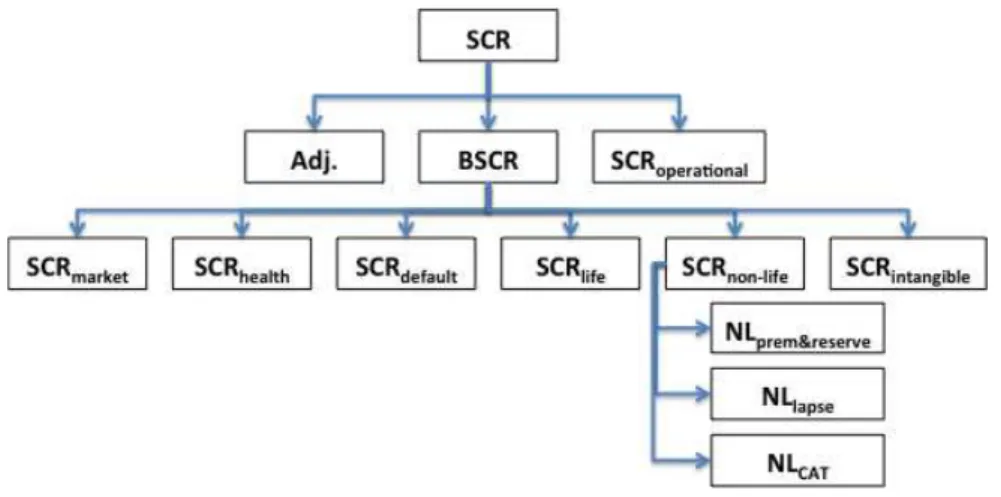
calculating this level of capital for all the undertakings and it was calibrated to achieve the target criteria of 99.5% Value-at-Risk for 1 year of time-horizon. It presents a modular structure as shown in the figure bellow:

Figure 2: SCR modular structure

3.1. Non-life underwriting risk

CEIOPS (2009a) provides advice and guidance on the methods, assumptions and standard parameters to be used in the design of the non-life underwriting

risk module, as required in Article 111(c) of Directive 2009/138/EC and has its legal support in Articles 111, 101, 104 and 105 of the Directive.

Although the risk of interest for the purpose of this report is the reserve risk, the

calculations for the combined premium risk and reserve risk will be presented in order to understand how the two risks interact in the standard formula. Premium

risk calculations will be detailed only when necessary to understand the reserve risk calculations.

3.2. Non-life premium and reserve risk sub-module

The capital charge for premium and reserve risk (NLpr) is given by:

V NL_pr =ρ(σ)⋅

where:

V = volume measure

σ = combined standard deviation, resulting from the combination of the reserve and premium risk standard deviations, and

1 1 ) ) 1 log( exp( ) ( 2 2 995 . 0 − + + ⋅ = σ σ σ

ρ N .

N0.995 = 99.5% quantile of the standard normal distribution

Note that ρ(σ) is computed assuming a log-normal distribution of the

underlying asset and an expected value of 1 in order to be consistent with the

To calculate the volume measure and the combined standard deviation it is necessary to calculate them for each individual LoB and for both premium risk

and reserve risk, and then aggregate them using the formulae bellow. For the volume measure we have

V= V_(prem,LoB)

LoB

∑

LoB

∑

V

(res,LoB)=PCOlob Where:

V(prem,LoB),V(res,LoB)= volume measure for premium and for reserve risk.

σ(prem,LoB), σ(res,LoB)=standard deviation for premium and for reserve risk.

PCO_{lob = best estimate for claims outstanding for each LoB.}

As the Advice states, «the standard deviation for premium and reserve risk for each LoB is defined by aggregating the standard deviations for both sub-risk under the assumption of a correlation coefficient of α_=0.5.»

σ_(lob)= (σ(prem,lob)V(prem,lob)) 2

+2ασ_(prem,lob)σ_(res,lob)V_(prem,lob)V_(res,lob)+(σ_(res,lob)V_(res,lob))2)

V_(prem,lob)+V_(res,lob)

Finally, the overall standard deviation is given by:

∑

r V V

CorrLob

V σ σ

σ 1_{2 ,}

where

r,c = all indices of the form (LoB)

CorrLobr,c = the correlation coefficient between LoB r and LoB c

The correlation matrix CorrLob structure is presented and explained in QIS3 - CEIOPS (2007) - which the CEIOPS’ Advice on non-life underwriting risk

3.3. Standard Parameter for Reserve Risk

CEIOPS (2010b) explains how the reserve risk calibration was performed,

identifying the data used, the assumptions considered and detailing the six different methods applied to calibrate the reserve risk to each LoB.

For the LoB Motor, vehicle liability, the data sample included data from 327

undertakings and from 106 undertakings for LoB Motor, other classes, in both cases gross of reinsurance. The different methods were applied to the collected

data.

For Motor, vehicle liability methods 1 and 2 provided a relatively poor fit but with some credibility in the tail, while method 4 gave significantly lower factors

than all the other methods. Therefore, the technical factor was chosen as the average of methods 1, 2, 3, 5 and 6, leading to the standard parameter for

reserve risk of 11%.

For Motor, others methods 1 and 2 provided a relatively poor fit and again method 4 gave significantly lower factors than all the other methods. Therefore

the technical factor was chosen as the average of methods 1, 5 and 6, leading to the standard parameter for reserve risk of 20%.

In the next chapters, different methods will be used to estimate the undertaking specific parameters for these two LoB, that would eventually substitute the 11% and the 20% in the standard formula, for vehicle liability and other classes,

respectively.

In order to do so, the CEIOPS’ Advice on technical provisions – CEIOPS

standards for data quality, in terms of appropriateness, completeness and accuracy of data.

Furthermore, the same applicable assumptions considered for reserve risk calibration in CEIOPS (2010b) were applied in this analysis, namely:

• Expenses are not considered in the run-off triangles used to derive the reserve risk standard deviation but are included in the reserve best estimate in the standard formula. Expenses are expected to be less

volatile than the claims and as result applying the estimate for reserve risk to both claims and expenses reserves is being conservative;

• No explicit allowance was made for inflation; it was assumed that inflationary experience in the period 2000 to 2012 was representative of

the inflation that might occur.

In order to obtain 100% credibility for the parameters estimates, the number of

years of historical data to be used is at least 15 for vehicle liability and 10 for other classes – see CEIOPS (2010a). However, It must be assured that data from each year is coherent and comparable; otherwise the results may prove

meaningless.

Due to relevant changes in the company’s claims handling and settling

4. M

R

R

E

When performing the ORSA exercise, (re)insurers are expected to define their overall solvency needs, which implies the choice of a relevant time horizon.

While the quantitative requirements are related to the first pillar of the directive and therefore to a 1-year time horizon, the forward looking perspective within ORSA requires to look beyond this period.

Accordingly we can consider:

• Single-period solvency – in the regulatory sense, having enough own funds to avoid economic bankruptcy over 1 year with a 99.5% threshold;

• Multi-year solvency – having enough own funds to avoid economic bankruptcy over the whole time horizon with a p threshold.

The reserve risk estimation was first approached in a multi-year perspective, by applying different stochastic methods to estimate the ultimate reserve risk

parameter.

Then the analysis was shortened to the one-year time horizon for the specific

purpose of obtaining the USP.

4.1. Setting up the model

Let us consider that annual data is available. Different periods of time may be considered with the respective adjustments in the notation and formulae.

Cik – accumulated total claims amount of accident year i, i=1, 2, …, I , either

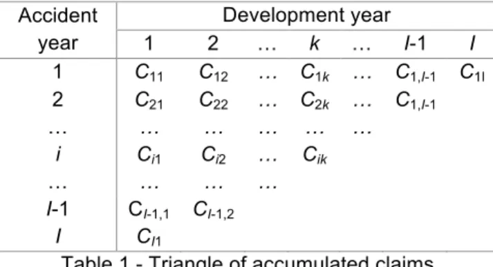
The set of available data can be grouped as follows:

Accident year

Development year

1 2 … _k … _{I-1 I}

1 C11 C12 … C1k … C1,I-1 C1I 2 C21 C22 … C2k … C1,I-1

… … … … … …

i Ci1 Ci2 … Cik

… _{… … …}

I-1 CI-1,1 CI-1,2

I CI1

Table 1 - Triangle of accumulated claims

For the purpose of estimating the reserve risk, tails in the run-off triangles were not considered. It was assumed that the tail has the same estimated variability.

The chain-ladder method is the basis for the methods that will be considered, therefore let us summarize the method for obtaining a deterministic estimation of the reserves:

i. Estimate the chain ladder development factors:

ˆ

f_k = i=1Ci,k+1

I−k

∑

C_i,k i=1

I−k

∑

k=1,…,I-1

ii. Obtain the estimation for the accumulated claims in the lower triangle of the claims data:

ˆ

Ci,I−i+2=Ci,I−i+1fˆI−i+1 , i=2,…,I

ˆ

C_i,k+1=Cˆikfˆk , i=3,…, I and k=I-i+2, I-i+3,…, I-1

iii. Estimate the outstanding claim reserve for accident year i=2,…,I_:

ˆ

R_i=Cˆ_iI−C_i

,I+1−i iv. The total outstanding claim reserve is given by:

ˆ

R₌ Rˆ

i i=2 I

4.2. Stochastic methods for ultimate reserve risk

This chapter presents three stochastic models for claims reserving and reserve

risk estimation: Mack’s model, Munich Chain Ladder model with an appropriate bootstrap simulation technique and the bootstrap simulations for the pure Chain

Ladder algorithm.

4.2.1. Mack’s Model

Mack (1993) presents a distribution-free formula for the standard error of the

chain ladder estimates, by considering the first two moments for the cumulative payments.

Mack’s assumptions:

• E(Ci,k+1Ci1,...,Ci,k)=Ci,kfk , i=1,…,I and k=2,…,I;

• there is no dependency between accident years;

• Var(C_i

,k+1Ci₁,...,Ci_,k)=Ci_,kσk

2

, i=1,…,I and k=1,…,I-1, where σk

2 _{can be}

estimated as follows: σˆ_k2

= 1

I−k−1 Cik

C_i,k+1

Cik −fˆ_k

"

#

$ %

& '

2

i=1

I−k

∑

For the last development year there is not enough data, therefore σˆ_I2_{−1 is}

computed in a different way. For the purpose of this work, it was used the

Under the assumptions above, it can be shown that the mean squared errors are:

mse( ˆR_i)=Cˆ2

iI

ˆ

σ_k2 ˆ

fk

2 1 ˆ

C_ik +

1

C_jk j=1

I−k

∑

k=I+1−i I−1

∑

mse( ˆR)=

(

)

j=i+1

I

∑

2σˆk

2 ˆ fk 2 Cnk n=1

I−k

∑

I−1

∑

∑

4.2.2. Bootstrap for Chain Ladder

The Bootstrap technique presented in Efron and Tibshirani (1993), is a simple but powerful technique to obtain information from one single sample of data. Assuming the observable data to be independent and identically distributed, the

generated sets of pseudo-data are consistent with the underlying distribution of the observed data. Therefore, statistics of interest can be obtained.

Generically, the methodology consists in sampling with replacement from the observed data sample, in order to obtain a sufficient number of sets of pseudo-data.

England and Verral (1999) present a relevant application of the bootstrap to obtain the estimation error of reserve estimates from the Chain-Ladder model.

Very often, data are not identically distributed, since the means and/or variances may depend on covariates, therefore it is common to resample residuals instead, which are usually independent and identically distributed or

England and Verral (2002) suggest the following bootstrap procedure:

- Obtain the standard chain-ladder development factors from cumulative

data;

- Obtain cumulative fitted value for the past triangle;

- Obtain incremental fitted values, mˆ_{ik, for the past triangle by differencing;}

- Calculate the unscaled Pearson residuals for the past triangle:

r_ik(P)₌Cik−mˆik ˆ

m_ik

- Estimate the Pearson scale parameter ϕ, by:

ˆ

φ=

r

ik

(P)

( )

i,kI−i+1

∑

1

2

I₍I₊₁₎₋₂I₊₁

- Adjust the Pearson residuals using:

r_ikadj= I

1

2I(I+1)−2I+1 ×r_ik(P)

- Begin the iterative loop, to be repeated N times:

i. Resample the adjusted residuals with replacement, creating a new past triangle of residuals;

ii. For each cell in the past triangle, obtain a set of pseudo-incremental data by solving the unscaled Pearson residuals in order to Cij, i.e.

C_ik =mˆ_ik+r_ik(P). mˆ_{ik ;}

iii. Create the corresponding set of pseudo-cumulative data;

v. Obtain from iv) the future triangle of incremental payments by

differencing. This values will be used as the mean, _m

ij, when simulating the process distribution;

vi. For each future payment cell (i,j), simulate a payment from the

process distribution with mean _m

ij and variance φˆmij;

vii. Sum the simulated payments in the future triangle by origin year and

overall to give the origin year and the total reserve estimates respectively;

viii. Store the results, and return to the start of the iterative loop.

The standard deviation of the stored results gives an estimate of the prediction error.

Sometimes, the residuals after adjustment may still have inherited skewness of

the original data. In these situations the bootstrap procedure presented above can be misleading since it uses an approximation to the normal distribution. Pinheiro et al. (2003) deal with this situation by introducing an extra step to the

bootstrap procedure.

4.2.3. Bootstrap for Munich Chain Ladder

Quarg and Mack (2004) present a new approach to claims reserving methodologies, that aims at reducing the gap between IBNR and IBNER (Incurred But Not Reported and Incurred But Not Enough Reported,

which are often far different from each other. For practical reasons, companies tend to choose one of the run-off triangles, ignoring the result that would be

obtained if the other run-off triangle would be used.

This approach assumes that Mack’s model is applicable to both paid and incurred losses triangles and it shows that commonly there are positive

correlations between paid and incurred losses that are ignored and that should be taken into account in the reserving process.

Instead of performing two separate chain ladder calculations (SCL), the Munich Chain Ladder (MCL) combines the paid-loss (P) and incurred-loss (I) data types by taking (P/I) and (I/P) ratios into account when doing projections.

The point of MCL is to estimate individual development factors f_ik that are

different for each origin and development year, as an alternative for a common

factor for each development year fk. Using the observed correlations between

the two run-off triangles, the first diagonal is projected for both triangles. The

next diagonals are projected with the implicit projected correlation of the last diagonal and the process is repeated recursively until the last cell of each

triangle has been projected.

The application of this method to different data sets, including the data sets used for this work, shows evidence that the MCL projections for paid and

incurred losses result in closer values than the SCL projections, which is to say that using MCL we obtain P/I ratios closer to 100% (in the long run we expect to

pay all and not more than the incurred losses).

corrections, either increases in the incurred loss as a result of underestimated case reserves or reductions as a result of overestimated case reserves. These

systematic corrections will inadequately influence the P/I and the I/P ratios, thus applying the method will result in meaningless projections.

Steps for MCL application:

i. As initial data, consider the triangles of paid and incurred data with the

same structure as presented in Table 1;

ii. For each run-off triangle, calculate the development factors and the standard deviation parameters as in Mack’s Model;

iii. Calculate for each development year the observed P/I and I/P ratios; iv. Adjust the observed paid losses with the observed I/P ratios and the

incurred losses with the observed P/I ratios, for the respective development year and then obtain their standard deviations (ρP and ρI

respectively);

v. Compute the conditional residuals for P, I, P/I and I/P, using the parameters σP, σI, ρPand ρI;

vi. Using the residuals of the P and I/P triangles draw the paid residual plot and obtain the correlation (λP), similarly, with the I and the P/I triangle draw the incurred plot and obtain it’s correlation (λI_);

vii. Recursively, using the estimated correlations, correct the development factors for the next development year and project the next diagonal of

For detailed explanation and formulae see Quarg and Mack (2004).

The steps above allow us to obtain deterministic projections for the ultimate

reserves, using paid and incurred losses. However, for the purpose of the present work, it is still necessary to estimate the risk implicit in this method. Liu and Verral (2010) present a bootstrap approach to estimate the predictive

distributions of reserves produced by the MCL, by applying bootstrapping methods to dependent data and consequently taking correlations into account.

Considering the categorization of the models introduced by England and Verral (2007) into recursive and non-recursive, since the MCL is a recursive model, Liu and Verral follow their approach of bootstrap for recursive models.

However, since we are dealing with two sets of correlated data, independence assumption is not met and therefore the normal bootstrap technique cannot be

used. The correlation observed in the data represents real dependence between the paid and incurred claims and it should remain unchanged within any resampling procedure.

Bootstrap Algorithm for MCL

After applying the MCL method to obtain the residuals for the four data sets, adjust the Pearson residual estimates to correct the bootstrap bias and group all four adjusted residuals together.

Then start the iterative loop to be repeated N times (N≥10000), consisting of the following steps:

of this bootstrap methodology as it allows to generate pseudo samples of the four residuals that reflect the same correlation structure from the

observed data;

ii. Calculate the pseudo samples of the four triangles by inverting the Pearson residuals;

iii. Compute the CPi,j and CIi,j weighted averages of the bootstrap paid and

incurred development factors, where CPi,j and CIi,j are the paid and

incurred losses for origin year i and development year j, respectively; iv. Obtain the corresponding correlation coefficient for the resampled data

using the pseudo residuals;

v. Calculate the variances for the bootstrap data;

vi. Compute the bootstrap development factors adjusted by the correlation

coefficient between the pseudo data for the resampled bootstrap paid and incurred run-off triangles;

vii. Recursively, simulate a future payment for each cell in the lower triangle

for both paid and incurred claims, from the process distribution with the mean and the variance obtained in vi), assuming a normal distribution;

viii. Sum the simulated payments in the future triangle by origin and overall, to obtain the origin year and the total reserve estimates, respectively; ix. Store the results and return to the start of the iterative loop;

4.3. Methods for one-year reserve risk

For the 1-year reserve risk, CEIOPS (2010a) details the three different methods that are currently accepted for purposes of USP estimation.

4.3.1. Method 1

This method assumes that the variance of the best estimate for claims outstanding in one year plus the incremental claims paid over the one year is

proportional to the current best estimate for claims outstanding.

It essentially consists in reviewing the run-off of the claims reserves based on

the undertaking’s data of historical claims provisions and payments, requiring at least five years of covered data, in order to compare the claims provision at the start of a financial year with the sum of the undertaking’s own claims provision

at the end of the financial year plus claims paid during that same year, and from there obtain an estimate for the constant of proportionality.

Lets first consider the following relationships:

V_Y,lob = PCOlob,i,j i+j=Y+1

∑

RY,lob= PCOlob,i,j i+j=Y+2

j≠1

∑

j≠1

∑

where:

V_Y

PCO_lob,i,j= Best estimate for claims outstanding by LoB for accident year i and

development year j.

R

Y,lob= Best estimate for outstanding claims and incremental paid claims for the exposures covered by the volume measure, but in one year’s time by calendar

year and LoB.

I_lob,i,j= Incremental paid claims by LoB, for accident year i and development

year j.

The behaviour of losses is formulated as:

lob Y lob lob Y lob Y lob

Y V V

R

, ,

,

, = + β ε ,

where:

βlob

2 _{= Constant of proportionality for the variance of the best estimate for claims}

outstanding in one year plus the incremental claims paid over the one year by LoB.

εY,lob= An unspecified random variable with distribution with mean zero and unit

variance.

The estimator forβlob is then:

ˆ

βlob= 1

N_lob−1 (R_Y

,lob−VY,lob) 2 V_Y ,lob Y

∑

N_{lob= The number of data points available by LoB where there is both a value}

of VY,lob and RY,lob.

Note that in this formulae R_Y

σ(U,res,lob) =

ˆ

βlob PCO_lob ,

where:

PCO_{lob=The best estimate for claims outstanding by LoB.}

This method tends to produce a higher USP factor when observed claims run-off is different from that initially expected. Moreover, it produces a USP factor

that will be applied to future reserves, therefore it’s only valid if the claims reserving methodology (implicit in the historical data use for the estimation) was the same along the years used for the estimation and if it remains the same in

the future.

4.3.2. Method 2

The second method is based on the mean squared error of prediction (MSEP) of the claims development result over a one-year time horizon using the

Merz-Wüthrich method presented by Merz and Merz-Wüthrich (2008).

In this method, the reserve risk factor is calculated as the square root of the estimated mean squared error, divided by the undertaking’s own claims

provision:

σ₍U,res,lob) =

MSEP

PCO_lob

The use of this method is only possible when the claims triangle is consistent with the Merz-Wüthrich model assumptions.

4.3.3. Method 3

This method is similar to method 2, except that the square root of the estimated mean squared error is now divided by the outstanding claims reserve estimated

using a chain-ladder projection method:

σ₍U_,res_,lob₎=

MSEP

CLPCO_lob

Where CLPCOlob is the best estimate for claims outstanding estimated using the chain ladder method applied to paid claim developments.

Method 3 produces a higher risk factor than method 2 when the undertaking’s

own claims provision is higher than the provision implied by a chain-ladder projection. Conversely, if the undertaking’s own claims provision is lower than the provision implied by a chain-ladder projection, then method 2 is the one that

produces a higher risk factor.

From a theoretical perspective Method 3 is more adequate then 2, because it

applies an estimate of the MSEP that was developed specifically for the pure chain ladder method, therefore, applying it to a different model might not reflect correctly the actual reserve risk. However, the final use of the reserve risk factor

5. A

M

,

V

L

M

,

O

The different models and methods presented in the previous chapters were applied to the company’s data for these two lines of business.

Information on claims payments and case reserves, both net of reimbursements, by origin and development year, for accidents occurred from

2000 to 2012, was collected and treated using the software SAS Enterprise

Guide and Microsoft Excel.

Due to the different behaviors of sub-lines of business and in order to obtain

more accurate values to the ultimate reserve risk, data was collected separately. LoB Motor, Vehicle Liability was separated in Bodily Injury (BI),

Material Damages (MD) and IDS – accidents that follow the direct compensation to the policy holder system. LoB Motor, others was separated in Own Damage and Passengers.

For the one-year reserve risk, data is to be considered grouped by the two lines of business, for consistency with the approach used in CEIOP’s documents.

The application of the theoretic models present in the previous chapters was performed using the statistical software R for Windows GUI front-end. Additional calculations and the implementation of the capital charge

calculations were performed using Microsoft Excel.

In order to preserve the confidentiality of the data, this chapter will only present

5.1. Results: Ultimate Reserve Risk

For the estimation of the ultimate reserve risk, a great use of the R® package ‘ChainLadder’ was done.

This package has implemented several functions for claims reserving, namely the Mack’ Model, the MCL Model and the Bootstrap for Chain Ladder:

- MackChainLadder – based on Mack (1993) and Mack (1999); - BootChainLadder – based on England and Verral (2002); - MunichChainLadder – based on Quarg and Mack (2004).

The use of these functions is exemplified in Annex 2.

The bootstrap procedure used for projections obtained via the MCL method

was fully implemented as can be seen in Annex 3.

When applying these methods to the data available, two relevant situations were detected:

- Bodily injury: the correlation between payments and incurred claims was negative. This is due to prudent case reserve estimates that are later

reduced, resulting in reduction of claims incurred while payments continuously increase. As a consequence, the MCL method is not applicable, since it assumes and uses the positive correlation between the two data sets to approximate the resulting projections.

- Own Damage: a couple of cells in the incremental payments, in the last developments years are negative due to some reimbursements.

The residuals distribution and the correlations obtained by the MCL method can be found in annexes 4 to 8.

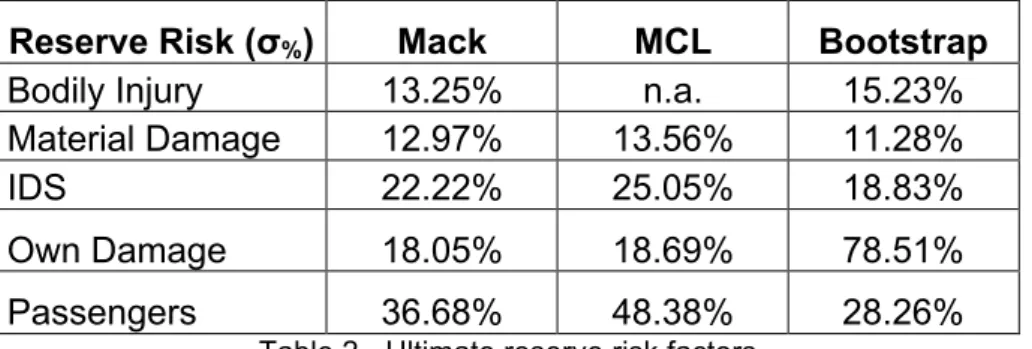
The overall results obtained are presented in the tables bellow.

Reserve Risk (σ_{%) Mack MCL Bootstrap}

Bodily Injury 13.25% n.a. 15.23% Material Damage 12.97% 13.56% 11.28%

IDS 22.22% 25.05% 18.83%

Own Damage 18.05% 18.69% 78.51% Passengers 36.68% 48.38% 28.26%

Table 2 - Ultimate reserve risk factors

The Bootstrap procedure shows the lower factors, except for Bodily Injury and

Own Damage for the reasons mentioned above.

On the other hand, as expected, the MCL produces higher factors. The MCL

ultimate projections are usually lower than the ones obtained in the other methods and the standard deviation is not lower enough to compensate, so the ratio – our reserve risk – is higher.

The Passengers data has a smaller size therefore the respective run-off triangle may not be sound enough to produce meaningful results.

5.2. Results: One-year Reserve Risk

The one-year reserve risk estimation should be performed using the claims payments run-off triangles for two data sets: vehicle liability and other.

Method 1 was computed as indicated in CEIOPS (2010a), using 8 years of historical data grouped for the two data sets. An example of the data used is

illustrated in Annex 9.

However, for Method 2 and 3 a different approach was taken.

Given two claims run-off triangles, their chain-ladder projections only add up to

the projections of the combined triangle under some specific conditions discussed by Ajne (1994). Additionally, Ajne (1994) presents sufficient

conditions for inequality between the combined projection vector and the sum of the two original projections vectors.

For Motor, others, considering the combined run-off results in approximately the

same reserves as adding up the reserves for Own Damage and Passengers. However the same doesn’t apply to Motor, vehicle liability, mainly due to the

different patterns of Bodily Injury data when compared to Material Damage and IDS data.

Bodily Injury has a longer tail and the payments volume has a smaller weight in the first developments years. This is sufficient condition for the chain-ladder

projections of the combined portfolio to be significantly less than the sum of the corresponding projections of the individual data sets (Theorem 2 in Anje (1994)).

The correlations were estimated from the ultimate reserves for each origin year, resulting in correlations of 0.62, 0.07 and -0.43 for BI and MD, BI and IDS and

MD and IDS, respectively.

To apply method 2 and 3 it was necessary to calculate the MSEP using the Merz-Wüthrich method (see Annex 10).

While method 3 uses the best estimate for claims outstanding obtained via Chain Ladder – which is to say via Mack’s model –, method 2 considers the

best estimate obtained using other methods, namely the MCL.

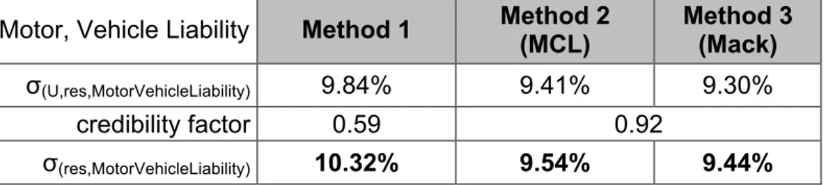
The results follow calculations in section 2.2.3. and are presented below.

Motor, Vehicle Liability Method 1 Method 2 (MCL)

Method 3 (Mack)

σ_{(U,res,MotorVehicleLiability)} 9.84% 9.41% 9.30%

credibility factor 0.59 0.92

σ_{(res,MotorVehicleLiability) 10.32% 9.54% 9.44%}

Table 3 - One-year reserve risk factors for LoB Motor, Vehicle Liability

Motor, Others Method 1 Method 2 (MCL)

Method 3 (Mack)

σ_{(U,res,MotorOthers)} 20.40% 16.88% 15.64%

credibility factor 0.81 1.00

σ_{(res,MotorOthers) 20.32% 16.88% 15.64%}

Table 4 - One-year reserve risk factors for LoB Motor, Others

The estimates obtained are to be compared with the standard parameters of 11% and 20% for Motor, Vehicle Liability and Motor, Others, respectively. Since

Method 1 produces higher factors than the other methods, in both cases very close to the standard parameters.

Method 2 and Method 3 origin factors are close and significantly better that the standard parameters, being slightly higher when using MCL best estimates. As a reference the Portuguese Regulator estimates for the Portuguese

undertakings 13.2% for Motor Vehicle Liability and 16.9% for Motor Other, considering a simple average of the estimates obtained for each undertaking, or

10.0% and 12.9% respectively, if considering a weighted average.

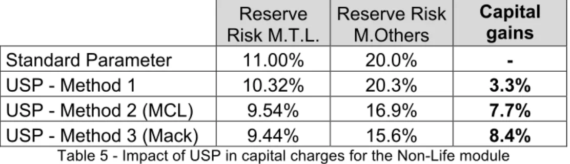
In terms of capital requirements (section 3.2.), the impacts are as follows:

Reserve Risk M.T.L.

Reserve Risk M.Others

Capital gains

Standard Parameter 11.00% 20.0% -

USP - Method 1 10.32% 20.3% 3.3%

USP - Method 2 (MCL) 9.54% 16.9% 7.7%

USP - Method 3 (Mack) 9.44% 15.6% 8.4%

Table 5 - Impact of USP in capital charges for the Non-Life module

USP calculated with method 1 has a smaller impact. The factor for Motor, Other is slightly higher than the standard but the one for Motor, Vehicle liability is lower than the standard and the best estimate for claims outstanding weights

more in the total best estimate, resulting in a gain of capital of 3.3%.

The gains with method 2 and 3 are considerably higher, representing around

8.4% for method 3 and 7.7% for method 2.

Different correlations were tested. In a pessimistic scenario (0.8 for BI and MD, 0.15 for BI and IDS and independence for MD and IDS) the capital gains were

6. C

F

D

The aim of this work was to understand the impact that the undertaking specific

parameters may have in Solvency II capital requirements for LoBs Motor Vehicle Liability and Motor Others.

The Directive and all the documentation supporting ORSA and the USP

confirmed the complexity and extent of this project.

The literature on claims reserving is much diversified but due to time limitations,

it was necessary to focus on a restrict number of methods. Therefore the methods more commonly used and more explored were the ones selected. The results obtained seem to support the intuitive idea that using USP actually

results in capital gains for the company, however the use of an USP has to go over an approval process from the regulator. The company must select the

method that believes to be more adequate to its own data and the selection of a particular method has to be explained to the regulator. The regulator needs evidence that the USP better reflects the company’s risk profile.

Across this work some aspects had to be simplified, however they should be analysed more carefully in the future. Further developments for this work would

be:

1. To consider a tail in the run-off triangles and in the reserve risk estimation. In this work, it was assumed that the tail has the same estimated variability;

A

Annex 1. CorrLob – Matrix of correlations between LoBs

CorrLob 1 2 3 4 5 6 7 8 9 10 11 12

1: Motor vehicle

liability 100% 50% 50% 25% 50% 25% 50% 25% 50% 25% 25% 25%

2: Other motor 50% 100% 25% 25% 25% 25% 50% 50% 50% 25% 25% 25%

3: MAT 50% 25% 100% 25% 25% 25% 25% 50% 50% 25% 25% 50%

4: Fire 25% 25% 25% 100% 25% 25% 25% 50% 50% 50% 25% 50%

5: 3rd party liability 50% 25% 25% 25% 100% 50% 50% 25% 50% 25% 50% 25%

6: Credit 25% 25% 25% 25% 50% 100% 50% 25% 50% 25% 50% 25%

7: Legal exp. 50% 50% 25% 25% 50% 50% 100% 25% 50% 25% 50% 25%

8: Assistance 25% 50% 50% 50% 25% 25% 25% 100% 50% 50% 25% 25%

9: Miscellaneous. 50% 50% 50% 50% 50% 50% 50% 50% 100% 25% 25% 50%

10:Np reins.

(property) 25% 25% 25% 50% 25% 25% 25% 50% 25% 100% 25% 25%

11:Np reins.

(casualty) 25% 25% 25% 25% 50% 50% 50% 25% 25% 25% 100% 25%

12:Np reins. (MAT) 25% 25% 50% 50% 25% 25% 25% 25% 50% 25% 25% 100%

Source: QIS5 Calibration Paper – CEIOPS (2010c) – page 354/3841

1

CEIOPS has also published a calibration paper which includes a description on the derivation of these correlations, which is available on CEIOPS’ website under

Annex 2. Using the R package ‘ChainLadder’

#################### ChainLadder Package######################### suppressPackageStartupMessages(library(ChainLadder))

#READING PAYMENTS

#In order to preserve the confidentiality of the data the paid and incurred triangles here #presented correspond to the data use by Quarg and Mack (2004)

PAID=matrix(c(576,1804,1970,2024,2074,2102,2131, 866,1948,2162,2232,2284,2348,NA,

1412,3758,4252,4416,4494,NA,NA, 2286,5292,5724,5850,NA,NA,NA, 1868,3778,4648,NA,NA,NA,NA, 1442,4010,NA,NA,NA,NA,NA,

2044,NA,NA,NA,NA,NA,NA),nrow=7,ncol=7,byrow=TRUE) #READING INCURRED COSTS

INC=matrix(c(978,2104,2134,2144,2174,2182,2174, 1844,2552,2466,2480,2508,2454,NA,

2904,4354,4698,4600,4644,NA,NA, 3502,5958,6070,6142,NA,NA,NA, 2812,4882,4852,NA,NA,NA,NA, 2642,4406,NA,NA,NA,NA,NA,

5022,NA,NA,NA,NA,NA,NA),nrow=7,ncol=7,byrow=TRUE) #Mack Model

Mack <- MackChainLadder(Triangle=PAID, est.sigma="Mack")

write.table(Mack$FullTriangle , file="MackFullTriangle.csv" , sep=";") #Ultimate projections write.table(Mack$Mack.S.E , file="MackSE.csv",sep=";") #Standard Error plot(Mack, lattice=TRUE)

#Munich Chain Ladder Model

MCL <- MunichChainLadder(PAID,INC, est.sigmaP="Mack",est.sigmaI="Mack")

write.table(MCL$MCLPaid , file="MCLDCPaid.csv" , sep=";") #Ult. projections Paid write.table(MCL$MCLIncurred , file="MCLDCIncurred.csv" , sep=";") #Ult. projections Incurred plot(MCL) #Results and paid/incurred residuals regression

#Bootstrap for Chain Ladder

Boot <- BootChainLadder(PAID,R=10000,process.distr=c("od.pois"))

Annex 3. Bootstrap for Munich Chain Ladder

#################### Bootstrap for Munich Chain Ladder ######################### #Continuing from Annex 2

nr=nrow(PAID);nc=ncol(PAID) #1-period factors, Q and Qinverse FP<-matrix(NA,nrow=nr,ncol=nc)

for(j in 1:nc) FP[,(j-1)]=PAID[,j]/PAID[,(j-1)] FI<-matrix(NA,nrow=nr,ncol=nc)

for(j in 1:nc) FI[,(j-1)]=INC[,j]/INC[,(j-1)] Q<-PAID/INC

QInv<-1/Q

############## Bootstrap #################### ##### 0. Obtaining the 4 residuals #####

PRes<-t(matrix(MCL$PaidResiduals,ncol=ncol(PAID),byrow=TRUE)) IRes<-t(matrix(MCL$IncurredResiduals,ncol=ncol(PAID),byrow=TRUE)) QRes<-t(matrix(MCL$QResiduals,ncol=ncol(PAID),byrow=TRUE))

QInvRes<-t(matrix(MCL$QinverseResiduals,ncol=ncol(PAID),byrow=TRUE)) ##### 1. Adjust the Pearson Residuals #####

#Calculating the adjustmet factors Adjust <- matrix(0,ncol=nr, nrow=nc)

for( j in 1:(nr-2) ) Adjust[,j] <- sqrt((nc-j)/(nc-j-1)) #Obtaining the adjusted residuals

AdjPRes <- PRes*Adjust AdjIRes <- IRes*Adjust AdjQRes <- QRes*Adjust AdjQInvRes <- QInvRes*Adjust

for (i in 1:nr){AdjQRes[i,(nr-i+1)]<-NA ;AdjQInvRes[i,(nr-i+1)]<-NA} ##### 2. Grouping the residuals #####

auxP <-matrix(AdjPRes[(AdjPRes!=0 & !is.na(AdjPRes)) ],ncol=1,byrow=TRUE) auxI <-matrix(AdjIRes[(AdjIRes!=0 & !is.na(AdjIRes))],ncol=1,byrow=TRUE) auxQ <-matrix(AdjQRes[(AdjQRes!=0 & !is.na(AdjQRes))],ncol=1,byrow=TRUE)

auxQInv <-matrix(AdjQInvRes[(AdjQInvRes!=0 & !is.na(AdjQInvRes))],ncol=1,byrow=TRUE) AllRes<-cbind(auxP,auxI,auxQInv,auxQ)

##### 3. LOOP ##### Nboot<-10000

originP<-matrix(NA,nrow=Nboot,ncol=nc) originI<-matrix(NA,nrow=Nboot,ncol=nc) totalP<-matrix(NA,nrow=Nboot,ncol=1) totalI<-matrix(NA,nrow=Nboot,ncol=1) for (N in 1:Nboot){

#Obtaining bootstrap residuals nres <- nrow(AllRes)

nsam <- (nc-1)*nc/2

auxiliar <- sample(1:nres,nsam,replace=T) ItRes<-matrix(0, nrow=nsam, ncol=4) for(i in 1:nsam){

ItRes[i,]<-AllRes[auxiliar[i],]

}

i<-1 while(i<=nc-j){ MatResP[i,j]<-ItRes[nsam-((nc+1-j)*(nc-j)/2)+i,1] MatResI[i,j]<-ItRes[nsam-((nc+1-j)*(nc-j)/2)+i,2] MatResQInv[i,j]<-ItRes[nsam-((nc+1-j)*(nc-j)/2)+i,3] MatResQ[i,j]<-ItRes[nsam-((nc+1-j)*(nc-j)/2)+i,4] i<-i+1 } }

#obtaining boostrap increment ratios MatRatiosP<-matrix(NA, nrow=nr, ncol=nc) MatRatiosI<-matrix(NA, nrow=nr, ncol=nc) MatRatiosQ<-matrix(NA, nrow=nr, ncol=nc) MatRatiosQInv<-matrix(NA, nrow=nr, ncol=nc) for(j in 1:(nc-1)){

i<-1 while(i<=nc-j){ MatRatiosP[i,j]<-(MatResP[i,j]*Mack$sigma[j])/sqrt(PAID[i,j])+Mack$f[j] MatRatiosI[i,j]<-(MatResI[i,j]*MackInc$sigma[j])/sqrt(INC[i,j])+MackInc$f[j] MatRatiosQ[i,j]<-(MatResQ[i,j]*MCL$rhoI.sigma[j])/sqrt(INC[i,j])+MCL$q.f[j] MatRatiosQInv[i,j]<- (MatResQInv[i,j]*MCL$rhoP.sigma[j])/sqrt(PAID[i,j])+MCL$qinverse.f[j] i<-i+1 } }

#obtaining bootstrap development factors

BootfP<-rep(0,nc);BootfI<-rep(0,nc);BootfQ<-rep(0,nc); BootfQInv<-rep(0,nc) sumP<-rep(NA,nc);sumI<-rep(NA,nc)

for(j in 1:(nc-1)){

sumP[j]<-colSums(PAID,na.rm=TRUE)[j]-PAID[nc-j+1,j] sumI[j]<-colSums(INC,na.rm=TRUE)[j]-INC[nc-j+1,j] i<-1 while(i<=nc-j){ BootfP[j]<- BootfP[j]+(PAID[i,j]/sumP[j])*MatRatiosP[i,j] BootfI[j]<- BootfI[j]+(INC[i,j]/sumI[j])*MatRatiosI[i,j] BootfQ[j]<- BootfQ[j]+(INC[i,j]/sumI[j])*MatRatiosQ[i,j]

BootfQInv[j]<- BootfQInv[j] + (PAID[i,j]/sumP[j])*MatRatiosQInv[i,j] i<-i+1

} }

#obtaining the bootstrap CORRELATION COEFFICIENTS

LambdaP<- sum(MatResQInv*MatResP,na.rm=TRUE)/sum(MatResQInv^2,na.rm=TRUE) LambdaI<-sum(MatResQ*MatResI,na.rm=TRUE)/sum(MatResQ^2,na.rm=TRUE)

#Obtaining the VARIANCES VarP<-rep(0,nc); VarI<-rep(0,nc); for(j in 1:(nc-2)){

i<-1 while(i<=nc-j){ VarP[j]<-VarP[j]+(PAID[i,j]*(MatRatiosP[i,j]-BootfP[j])^2)/(nc-j-1) VarI[j]<-VarI[j]+(INC[i,j]*(MatRatiosI[i,j]-BootfI[j])^2)/(nc-j-1) i<-i+1 } } VarQ<-rep(0,nc); VarQInv<-rep(0,nc) for(j in 1:(nc-1)){

i<-1

while(i<=nc-j){

i<-i+1 } } sigmaP<-sqrt(VarP) sigmaI<-sqrt(VarI) tauI<-sqrt(VarQ) tauP<-sqrt(VarQInv)

#estimating the last ratio sigma/tau sigtauP<-sigmaP/tauP

sigtauI<-sigmaI/tauI period<-c(1:nc)

fitP<-lm(log(sigtauP) ~ period,na.action=na.exclude) fitI<-lm(log(sigtauI) ~ period,na.action=na.exclude)

sigtauP[nc-1]<-exp((nc-1)*fitP$coefficients[2]+fitP$coefficients[1]) sigtauI[nc-1]<-exp((nc-1)*fitI$coefficients[2]+fitI$coefficients[1]) alphaP<-pmax(0,pmin(LambdaP*(sigtauP),0.99))

alphaI<-pmax(0,pmin(LambdaI*(sigtauI),0.99))

#Obtaining the bootstrap ADJUSTED DEVELOPMENT FACTORS BlambdaP<-matrix(NA, nrow=nr, ncol=nc)

BlambdaI<-matrix(NA, nrow=nr, ncol=nc)

BPAID<-PAID; BINC<-INC; BRatiosQ<-MatRatiosQ; BRatiosQInv<-MatRatiosQInv for(k in 1:(nc-1)){

j<-k while(j<=(nc-1)){ BlambdaP[nr-j+k,j]<-BootfP[j]+alphaP[j]*(BINC[nr-j+k,j]/BPAID[nr-j+k,j]-BootfQInv[j]) BlambdaI[nr-j+k,j]<-BootfI[j]+alphaI[j]*(BPAID[nr-j+k,j]/BINC[nr-j+k,j]-BootfQ[j]) BPAID[nr-j+k,j+1]<-BlambdaP[nr-j+k,j]*BPAID[nr-j+k,j] BINC[nr-j+k,j+1]<-BlambdaI[nr-j+k,j]*BINC[nr-j+k,j] j<-j+1 } }

#Obtaining normal distributed observations BPAIDfinal<-PAID; BINCfinal<-INC for(k in 1:(nc-1)){

j<-k while(j<=(nc-1)){ meanP<-BlambdaP[nr-j+k,j]*BPAIDfinal[nr-j+k,j] sdP<-sqrt(VarP[j]*BPAIDfinal[nr-j+k,j]) meanI<-BlambdaI[nr-j+k,j]*BINCfinal[nr-j+k,j] sdI<-sqrt(VarI[j]*BINCfinal[nr-j+k,j]) BPAIDfinal[nr-j+k,j+1]<-rnorm(1,mean=meanP,sd=sdP) BINCfinal[nr-j+k,j+1]<-rnorm(1,mean=meanI,sd=sdI) j<-j+1 } }

#Obtaining the origin year and the total amounts originP[N,]<-BPAIDfinal[,nc]

originI[N,]<-BINCfinal[,nc]

reservesI<-averI-c(2131,2348,4494,5850,4648,4010,2044) totreserveP<-sum(reservesP)

totreserveI<-sum(reservesI) #standard deviations

stdP<-rep(NA,nrow=1,ncol=(nc-1)) for(j in 1:nc-1)stdP[j]=sd(originP[,j+1]) stdI<-rep(NA,nrow=1,ncol=(nc-1)) for(j in 1:nc-1)stdI[j]=sd(originI[,j+1]) totstdP<-sd(totalP)

Annex 4. Plots for Bodily Injury

Standardized residuals

Fitted Origin Period

Calendar Period Development Period

Paid Residual Plot Incurred Residual Plot

Annex 5. Plots for Material Damage

Standardized residuals

Fitted Origin Period

Calendar Period Development Period

Paid Residual Plot Incurred Residual Plot

Annex 6. Plots for IDS

Standardized residuals

Fitted Origin Period

Calendar Period Development Period

Paid Residual Plot Incurred Residual Plot

Annex 7. Plots for Own Damage

Standardized residuals

Fitted Origin Period

Calendar Period Development Period

Paid Residual Plot Incurred Residual Plot

Annex 8. Plots for Passengers

Standardized residuals

Fitted Origin Period

Calendar Period Development Period

Paid Residual Plot Incurred Residual Plot