DOI: 10.1590/1808-057x201603220
he inluence of the 2008 inancial crisis on the predictiveness of
risky asset pricing models in Brazil*
Adriana Bruscato Bortoluzzo
Insper, Faculdade de Ciências Econômicas, Departamento de Métodos Quantitativos, São Paulo, SP, Brazil
Maria Kelly Venezuela
Insper, Faculdade de Ciências Econômicas, Departamento de Métodos Quantitativos, São Paulo, SP, Brazil
Maurício Mesquita Bortoluzzo
Universidade Presbiteriana Mackenzie, Programa de Pós-Graduação em Administração de Empresas, São Paulo, SP, Brazil
Wilson Toshiro Nakamura
Universidade Presbiteriana Mackenzie, Programa de Pós-Graduação em Administração de Empresas, São Paulo, SP, Brazil
Received on 02.18.2016 – Desk acceptance on 03.17.2016 – 2nd version approved on 08.18.2016
ABSTRACT
his article examines three models for pricing risky assets, the capital asset pricing model (CAPM) from Sharpe and Lintner, the three factor model from Fama and French, and the four factor model from Carhart, in the Brazilian market for the period from 2002 to 2013. he data is composed of shares traded on theSão Paulo Stock, Commodities, and Futures Exchange (BM&FBOVESPA) on a monthly basis, excluding inancial sector shares, those with negative net equity, and those without consecutive monthly quotations. he proxy for market return is the Brazil Index (IBrX) and for riskless assets savings accounts are used. he 2008 crisis, an event of immense proportions and market losses, may have caused alterations in the relationship structure of risky assets, causing changes in pricing model results. Division of the total period into pre-crisis and post-crisis sub-periods is the strategy used in order to achieve the main objective: to analyze the efects of the crisis on asset pricing model results and their predictive power. It is veriied that the factors considered are relevant in the Brazilian market in both periods, but between the periods, changes occur in the statistical relevance of sensitivities to the market premium and to the value factor. Moreover, the predictive ability of the pricing models is greater in the post-crisis period, especially for the multifactor models, with the four factor model able to improve predictions of portfolio returns in this period by up to 80%, when compared to the CAPM.
Keywords: CAPM, market anomalies, multifactor model, prediction, 2008 inancial crisis.
1 INTRODUCTION
he capital asset pricing model (CAPM), developed by Sharpe (1964) and Lintner (1965) has been the model that is most widely used by the market for calculating expected rates of return on risky assets. Although the CAPM calculates expected excess return on risky assets as the only function of their systematic risk, subsequent empirical studies indicate the existence of other factors that inluence achieved historic returns. Banz (1981) found evidence of greater historic records for small stock companies. Stattman (1980) showed that the average return on US shares is greater for value companies, or rather, those with a high book value of net equity to market value ratio (high book-to-market index [BM]). Based on these market anomalies, Fama and French (1993) proposed an empirical model in which they identiied three risk factors that would determine expected return on shares: the market factor, the factor related to the size of the irm, and another to the BM index. Subsequently, Carhart (1997) added a fourth factor, related to momentum, based on evidence from Jegadeesh and Titman (1993) regarding signiicantly positive historic returns from adopting a strategy of buying winning shares funded by the sale of losing shares. Garcia and Ghysels (1998) documented the importance of studying structural changes in emerging markets, and recently, articles that address estimating systematic risk in a dynamic way have gained more ground in the literature, since the structure of correlation between the factors involved in the models sufers from an alteration over time, especially when structural breaks exist in the time series, arising for example from a crisis period. Silva, Pinto, Melo, and Camargos (2009), Garcia and Bonomo (2001), Machado, Bortoluzzo, Martins, and Sanvicente (2013), and Tambosi Filho, da Costa, and Rossetto (2006) published papers that evaluated the eiciency of the conditional CAPM model (C-CAPM) proposed by Bodurtha and Mark (1991) in the Brazilian market. On the other hand, Lewellen and Nagel (2006) found empirical evidence that the results from the C-CAPM do not difer signiicantly from the results from the non-conditional CAPM, since the relationship between the betas and the market risk premium varies very smoothly
over time. his leads to the belief that in order for there to be signiicant changes in the asset pricing model coeicients, an event with greater intensity needs to occur in order to provoke an alteration in the dependency structure of the variables, such as a crisis.
he main aim of this article is to verify whether there was any alteration in the correlation structure of the single and multifactor model variables due to the occurrence of the 2008 crisis, that is, to examine the behavior of risk premiums in the Brazilian market in the periods before and ater the 2008 inancial crisis. To do so, the period from 2002 to 2013 was divided into three (pre-crisis, crisis, and post-crisis), and for the irst and last of these sub-periods, non-conditional single and multifactor models were estimated in order to compare the results in a descriptive way and using the Chow parameter stability test. he results from this test indicate the existence of signiicant diferences before and ater the crisis, both in the relationship between the factors and in the values and signiicance of the coeicients of the CAPM and of the three factor model from Fama and French and the four factor model from Carhart, which justiies the division of the sample into the sub-periods.
he paper also analyzes the predictive ability of each one of the models evaluated for the Brazilian market based on calculating the root mean square error (RMSE) and the mean absolute percentage error (MAPE), which are measures that compare observed return with the return estimated for the portfolios by a particular model. hese measures indicate the supremacy of the multifactor models in comparison with the CAPM in the two sub-periods analyzed, with the four factor model presenting slightly better performance than the three factor and all of the models presenting better predictions in the period following the 2008 crisis.
he next section describes the single and multifactor models, their variables, and expected results, and then an empirical literature review of studies of the Brazilian market is carried out. Finally, the results from the models are presented, analyzed, and interpreted.
2 SINGLE AND MULTIFACTOR RISK MODELS
he CAPM, from Sharpe and Lintner, is a theoretical model that, according to Black, Jensen, and Scholes (1972), depends on the following hypotheses: (a) all investors are
costs exist; (c) all investors have information symmetry regarding the joint probability density function of returns on assets; (d) all investors can lend and borrow at a
risk-free rate. Under these hypotheses, the main result from the model indicates that:
E(ri) – rf = βi (E(rm) – rf)
in which E(ri) represents the expected return on a risky asset
i, rf is the return on a risk-free asset, E(rm) is the expected return on a portfolio representative of the market, and βi is the measure of sensitivity of the return from asset i to market return, representing the asset’s systematic risk coeicient.
Although Roll (1977) considers it to be impossible to test the CAPM empirically, alleging that no adequate proxy would exist for a market portfolio as deined by the model,
various authors (Banz, 1981; Carhart, 1997; Fama & French, 1993; Jegadeesh & Titman, 1993; Stattman, 1980) have found empirical evidence that the return on a risky asset depends on other risk factors that are not captured by the β of the asset. Unlike the CAPM, which is a theoretical model, the empirical three factor model from Fama and French (1993) aims to capture the sensitivity of return to other risk factors, and is represented by equation 2:
E(ri) – rf = bi(rm – rf) + si(SMB) + hi(HML)
in which E(ri) – rf is the expected excess return on portfolio
i, rm – rf is the excess return on the market portfolio,
SMB, meaning small minus big, or size factor, is the risk premium for maintaining a portfolio bought in shares in small companies and sold in shares in big companies, HML, meaning high minus low, or value factor, is the risk premium for maintaining a portfolio bought in shares in companies with a high BM index (value shares) and sold in shares with a low BM index (growth shares), and bi, si, and hi are the sensitivities related to the respective factors. Fama and
French (1993) considered the factors as proxies for risk factors. According to them, there is empirical evidence that the two factors are related to return; in other words, large companies or growth ones would have lower returns on assets when compared to small companies or with value companies, respectively. hus, it is expected that positive risk premiums will be found for each one of the three factors. Carhart (1997) adds the momentum factor (WML, or winners minus losers) to the three factor model, resulting in the four factor model:
E(ri) – rf = bi(rm – rf) + si(SMB) + hi(HML) + wi(WML)
in which WML is the risk premium for maintaining a portfolio bought in winning company shares (which obtained above average returns in the previous year) and sold in losing shares (which obtained below average returns in the previous year), and wi is the sensitivity of the portfolio with relation to the WML.
Just like the size and value factors, the addition of WML is empirically justiied. Vayanos and Woolley (2013) explain WML as a result of the gradual removal of funds invested in a discredited company. In a second phase, the capital low could be large enough for its market value to diverge too much from its fair value, at which point a reversal would occur. Jegadeesh and Titman (2001), however, veriied that the factor is neither consistent with the random walk hypotheses, nor with the inancial behavior hypotheses, since reversal only occurs in some of the sub-periods analyzed, with some anomaly thus being involved. he anomaly is characterized by a positive above-market return in the year
following the year in which the share was winning (even if there is a reversal, this takes place ater this period). hus, we expect a positive premium for WML.
To evaluate the predictive power of models (1), (2), and (3), time series regressions are carried out with the inclusion of the αi intercept, which must have its signiicance tested. As set out by Black et al. (1972), the αi term, also known as the Jensen alpha in its CAPM version, if statistically diferent from zero, indicates a violation of hypothesis (a) of the CAPM. As the other models also propose to explain the totality of excess return on well diversiied portfolios, the αi coeicient should be statistically equal to zero for the three models analyzed. If the model presents an intercept that is statistically above (below) zero for some portfolio, it means that that portfolio had a positive (negative) excess return ater controlling all of the risk factors in the model, and there is therefore evidence that, for that portfolio, some risk factor was not captured by the model.
1
2
3 MAIN EMPIRICAL EVIDENCE IN THE BRAZILIAN MARKET
Málaga and Securato (2004) obtained results that conirmed the superiority of the three factor model in relation to the CAPM in explaining returns on Brazilian shares. Mussa, Rogers, and Securato (2009) produced a paper in which they tested the predictive ability of the CAPM and the three factor model, carrying out the two stage procedure in accordance with Fama and MacBeth (1973) and concluded that neither of the two models is eicient in predicting returns on Brazilian shares, given the signiicance observed in the regression intercepts.
In another paper, Rogers and Securato (2009) carried out a study of the three factor model from Fama and French in the Brazilian market, comparing with the traditional single factor CAPM and the reward beta approach, and concluded that the multiple factor model was superior, however excluding accounting HML over market value, which was not shown to be statistically signiicant. he period covered was 1995 to 2006, subdivided into two sub-periods: one to estimate risk premiums and the other to test the models.
Mussa, Famá, and Santos (2012) carried out a study of the Brazilian equities market in which they tested the three factor model from Fama and French, as well as the four factor model proposed by Carhart, incorporating WML. he results from the study indicated the validity of including the four factors in the broadened version of the original CAPM, in which despite SMB and WML presenting a negative premium, contradicting the original studies from Fama and French (1993) in the case of SMB, and from Carhart (1997) in the case of WML, other results obtained for the Brazilian context were conirmed, such as that from Málaga and Securato (2004).
Argolo, Leal, and Almeida (2012) carried out a study regarding the three factor model from Fama and French with data from Brazil and covering the period from 1995 to 2007, that is, subsequent to the Brazilian currency stabilization plan and prior to the period that succeeded the subprime inancial crisis. he authors concluded that using the three factor model was statistically valid, incorporating a premium for
SMB and another for the so-called value stocks factor. hey veriied, therefore, that the three factor model has greater explanatory power compared to the single factor model, corresponding to the CAPM from Sharpe and Lintner. However, it was veriied that the historical averages of the HML and SMB premiums are very high and they did not present better estimates than the one factor traditional model for estimating the cost of equity capital in the Brazilian context.
Rayes, Araújo, and Barbedo (2012) tested the three factor model from Fama and French, considering in particular the structural break occurring in the Brazilian equities market as a result of the sharp increase in liquidity in mid-2006. hey selected 40 shares with higher liquidity in 2004 and traded on the stock exchange in the period from July 2000 to June 2008. Considering the shares both individually and combined in portfolios, they found that the SMB and HML factors do not explain market returns more, due to the structural break mentioned above.
In a more recent paper, Noda, Martelanc, and Kayo (2015) included the risk factor Price-to-Earnings Ratio in the traditional CAPM, verifying the validity of using this factor in explaining returns on Brazilian shares, covering the period from 1995 to 2014. he results from the study indicated that the greater the Price-to-Earnings Ratio, the greater the return on shares tends to be, complementary to the CAPM beta efect. his factor was shown to be signiicant even ater controlling for the other components of the three factor model from Fama and French.
In light of this, we can infer that there is not yet any clear evidence of the superiority of the three or four factor models, as well as that little evidence exists regarding the predictive ability of these models, at least for the context of the Brazilian equities market. he most recent articles do not address the crisis period speciically, which makes it impossible to verify the adjustment of the models in this period, in which a modiication occurs in the dependency structure of the data involved in the pricing models.
4 METHODOLOGY
he population analyzed comprises all non-inancial company shares listed on the São Paulo Stock, Commodities, and Futures Exchange (BM&FBOVESPA) between January 2002 and December 2013, with all of the secondary data collected from the Economatica information system. Shares in inancial sector companies were ignored, due to them presenting high debt ratios that inluence the BM multiple. In
composing the database, shares that had not been traded in any session in the analysis period were excluded. Companies that had more than one type of share had the least liquid ones excluded from the base. hese exclusions alone restricted the database to 253 shares.
were necessary: shares that did not present consecutive monthly quotations for the 12 month period ater the portfolio formation so that return on the shares can be calculated, shares that did not present consecutive monthly quotations for the 12 month period before the portfolio formation so that classiication between winners and losers is possible, and shares without a market value on December 31 of each year, and companies that do not have positive liquid equity on December 31 of each year.
hus, for each year, the sample had a diferent number of shares available for forming part of the portfolios. For example, for 2002, our sample presented 59 shares with available data, while in 2013 there were 207 shares with available data. On average, the sample had 127 shares with data available for composing the portfolios.
It is veriied that the use of the methodology proposed by Fama and French (1993) for forming portfolios results in portfolios with only one or two shares in some years, which violates the hypothesis that portfolios are diversiied, implying a high speciic risk component, which could undermine the statistical tests regarding the coeicients of the models analyzed. In order to eliminate the problem of lack of diversiication, common in less developed markets in which the number of companies listed is very small,
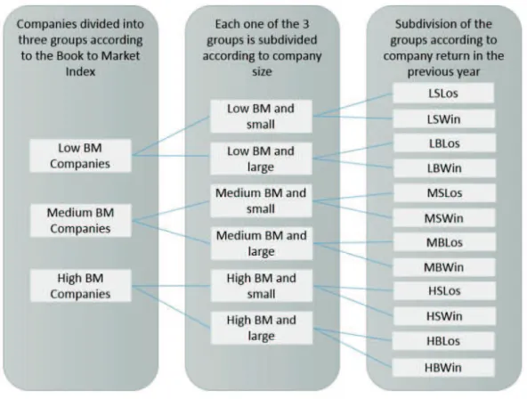
such as that of Brazil, this article uses the same alternative methodology for forming portfolios proposed in Rogers and Securato (2009) and described below. First, the shares are ordered by the BM index and divided into three groups with approximately the same number of shares in accordance with the percentages 30% and 70%; second, for each one of the three groups separately, the shares are ordered by their market value and each group is subdivided between small and large companies using the median of each group, resulting in six groups with approximately the same number of shares; in the third and last step, each one of the six groups is ordered separately in accordance with the previous year’s returns and subdivided into two more, between winning and losing shares, in accordance with the median of each subgroup. he logic of the method is illustrated in Figure 1. he diference in the method proposed is that the annual divisions of the groups are carried out using the percentages from the subgroups formed in the previous stage, whereas the Fama and French method uses the percentages from the total sample in each stage. Using the method proposed, it is guaranteed that each one of the portfolios has approximately the same number of shares in its composition and that all the portfolios are relatively well diversiied.
Figure 1 -Methodology for separating portfolios for emerging markets
BM: book-to-market index; L = companies with low BM; M = companies with medium BM; H = companies with high BM; B = big companies; S = small companies; Los = losers; Win = winners.
Despite the beneits of the methodology proposed, it only makes sense to use this alternative if the original variables BM, size, and return are weakly correlated so that it is guaranteed that, for example, a portfolio with small company has a lower market value than a portfolio with big company, as occurs in the proposal from Fama and French. In the period evaluated, the correlations were very weak in magnitude, lower that 0.09 for BM and return vs. size and lower than 0.3 in the case of return vs. BM, which makes the use of this type of modiication possible in compiling portfolios for the Brazilian market without causing bias in the portfolios formed. Moreover, we validated the construction
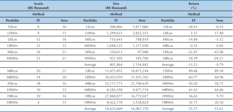
of portfolios using the modiied methodology observing average and standard deviation (SD) values from each portfolio for each one of the years from 2002 to 2013 and verifying the same ordering of portfolios by size and return, as in the Fama and French method. Table 1 shows the results obtained for the portfolios in 2013 in which it is observed, in the second column, that for the method proposed, as well as for the Fama and French method, all of the small company portfolios have a lower market value when compared with big company portfolios. It is also possible to observe that average size and average return have very close values between the two methodologies.
Table 1 -Quantity of shares, size, and return of portfolios formed in 2013 using the Fama and French (FF) method and with the
modiication proposed in this paper (New)
Assets (R$ thousand)
Size (R$ thousand)
Return (%)
Method Method Method
Portfolio FF New Portfolio FF New Portfolio FF New
LSLos 8 16 LSLos 500,866 1,817,066 LSLos -28.43 -0.55
LSWin 9 15 LSWin 1,299,633 2,823,315 LBLos 5.11 17.40
LBLos 12 16 MSLos 710,643 788,818 MSLos -14.84 -5.12
LBWin 33 15 MSWin 1,048,125 1,217,058 MBLos -0.35 0.85
MSLos 16 21 HSLos 330,613 97,088 HSLos -22.47 -43.08
MSWin 23 21 HSWin 921,305 185,708 HBLos -18.39 -28.21
Average 801,864 1,154,842 Average -13.23 -9.79
MBLos 20 21 LBLos 13,473,852 18,873,244 LSWin 89.68 89.50
MBWin 24 20 LBWin 20,453,979 31,931,765 LBWin 60.77 68.96
HSLos 38 16 MBLos 22,117,773 21,190,639 MSWin 50.20 58.72
HSWin 10 15 MBWin 8,285,358 9,477,719 MBWin 63.43 64.46
HBLos 10 16 HBLos 27,060,877 16,772,027 HSWin 36.65 9.70
HBWin 4 15 HBWin 8,422,178 3,558,824 HBWin 32.71 30.30
Average 16,635,669 16,967,370 Average 55.57 53.61
Note. HBLos = high book-to-market (BM) index, big, and loser companies; HBWin = high BM index, big, and winner companies;
HSLos = high BM index, small, and loser companies; HSWin = high BM index, small, and winner companies; LBLos = low BM index, big, and loser companies; LBWin = low BM index, big, and winner companies; LSLos = low BM index, small, and loser companies; LSWin = low BM index, small, and winner companies; MBLos = medium BM index, big, and loser companies; MBWin = medium BM index, big, and winner companies; MSLos = medium BM index, small, and loser companies; MSWin = medium BM index, small, and winner companies.
Source: Elaborated by the authors.
After compiling the portfolios, for each one of the methodologies time series regressions are carried out for models (1), (2), and (3), for the pre-crisis, post-crisis, and total periods. he inancial crisis from 2007 to 2009 was subdivided by Phillips and Yu (2011) into three burst bubbles, namely: the subprime crisis, from August to December 2007, the commodities crisis, from March to July 2008, and the bonds crisis, from September 2008 to April 2009. he subprime crisis was triggered in the United States of America and did not signiicantly afect the Brazilian market. By means of a graphic analysis of the Brazilian stock exchange index
it is veriied that it was only afected ater the commodities bubble burst so that the period between March 2008 and April 2009 was used to deine the crisis period. hus, the period before the crisis was deined as that between January 2002 and February 2008, and the post-crisis period as that between May 2009 and December 2013.
Index (IBrX) and savings accounts due to them being more consistent with the CAPM theory. he Ibovespa was an equities index weighted only by liquidity and came to be by the market value with a limit on participation based on liquidity, while the IBrX is an index of shares weighted only by the market value of shares and contains the 100 most liquid assets on the Brazilian exchange. It is worth
highlighting that the change in weighting criterion for Ibovespa shares only occurred ater the period covered in our sample. Savings accounts present a low DP and are accessible to any investor. heir use is justiied by Silva, Pinto, Melo, and Camargos (2009) and they are used in a recent study from Sanvicente (2014), among other papers.
5 RESULTS
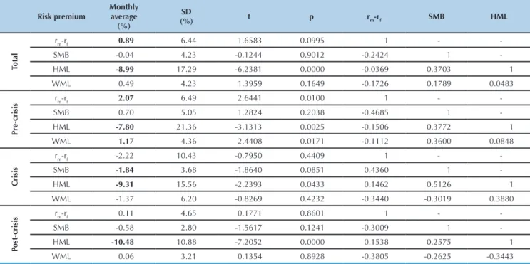
Tables 2 presents the risk premiums calculated for the period from 2002 to 2013 (total) and for the pre-crisis, crisis, and post-crisis sub-periods, as well as the correlation between the market factors, SMB, HML, and WML. It is veriied that the market risk premium for the whole sample was positive, as expected, and equal to 0.89% a month and statistically signiicant to 10%. his value is lower than those found by Sanvicente (2014), Machado and Medeiros (2011), Málaga and Securato (2004), and Mussa, Famá, and Santos (2012), which were 1.65%, 3.09%, 1.09%, and 1.56%, respectively, this being expected due to the long history of low market returns for the sample used in this paper, with the crisis and post-crisis periods.
Analyzing the sub-periods, it is important to highlight that the market risk premium is positive and signiicant only for the pre-crisis period, being negative in the crisis period and close to zero in the post-crisis period, but without statistical relevance in these last two sub-periods. It can also be noted that, in using the total sample in the time regression, the pre-crisis period predominates due to it having more observations, inluencing the regression coeicients. However, as suggested in Bortoluzzo, Minardi, and Passos (2014), and Sandoval Jr., Bortoluzzo, and Venezuela (2014), the short timeframe can more eiciently explain the relationship between risk and return. Alterations of this nature can be observed for the other factors, especially for SMB and WML.
SMB was statistically signiicant in the crisis period and its negative sign indicates that in this period the returns of large companies were greater than those of small companies, probably due to the liquidity problem of low market value companies. Although there is the expectation of higher returns for these companies in the long run, the reason for this premium would precisely be the diiculty in selling these shares at times of crisis or selling them with large negative variations in price, given the pressure to sell. Comparing the values for the pre-crisis and post-crisis periods, it is perceived that before the crisis this premium was positive, and ater it became negative, although not statistically signiicant.
HLM behaves in a more stable way over time; negative and statistically signiicant for all of the sub-periods, however a little lower in the post-crisis period, compared to the pre-crisis one. It is worth highlighting that the negative sign result
for Brazil is diferent from the result obtained by Fama and French (1993), indicating that the factor captures a diferent anomaly for Brazil in comparison to the US market. One possible explanation for this diference is that in the United States of America this factor is based on the existence of growth companies, in which the book value of assets is very small when compared with market value, such as in technology companies, which are intensive in intangible non-accounted assets. In Brazil, these companies would be those that have a consistent historic increase in valuation over the years, so that market value ends up exceeding book value; that is, in Brazil we do not have practically any technology companies listed on the stock exchange and companies classiied as growth companies are those that presented great increase in valuation in the study period, which results in high market value compared to net book value of equity. In our study, the companies that it this description were large consolidated groups. For example, Companhia de Bebidas das Américas (AMBEV), a company that in the US market would be considered as value due to a recent history of share appreciation, ended up being classiied as growth, and there are various other similar cases.
WML presented the expected sign, however with statistical signiicance in the pre-crisis sub-period only. In the post-crisis sub-period there was practically no diference between return on the assets of winning and losing companies, with a value close to zero that was not relevant. his fact reveals indications that the crisis may have caused some regime change not absorbed by the traditional pricing models.
remained this way ater the crisis; the relationship between the market and WML factors, which was negative and weak before the crisis and became moderate during and ater the
crisis; and the relationship between WML and SMB, which presented an alteration from a positive sign before the crisis to a negative sign in the post-crisis period.
Table 2 - Risk premiums in the period from 2002 to 2013 and in the pre-crisis, crisis, and post-crisis sub-periods
Risk premium
Monthly average
(%)
SD
(%) t p rm-rf SMB HML
Total
rm-rf 0.89 6.44 1.6583 0.0995 1 -
-SMB -0.04 4.23 -0.1244 0.9012 -0.2424 1
-HML -8.99 17.29 -6.2381 0.0000 -0.0369 0.3703 1
WML 0.49 4.23 1.3959 0.1649 -0.1726 0.1789 0.0483
Pr
e-crisis
rm-rf 2.07 6.49 2.6441 0.0100 1 -
-SMB 0.70 5.05 1.2824 0.2038 -0.4685 1
-HML -7.80 21.36 -3.1313 0.0025 -0.1506 0.3772 1
WML 1.17 4.36 2.4408 0.0171 -0.1112 0.3600 0.0848
Crisis
rm-rf -2.22 10.43 -0.7950 0.4409 1 -
-SMB -1.84 3.68 -1.8640 0.0851 0.4360 1
-HML -9.31 15.56 -2.2393 0.0433 0.1462 0.5126 1
WML -1.37 6.20 -0.8269 0.4232 -0.3440 -0.3019 0.3880
Post-crisis
rm-rf 0.11 4.65 0.1771 0.8601 1 -
-SMB -0.58 2.80 -1.5617 0.1241 -0.3009 1
-HML -10.48 10.88 -7.2052 0.0000 0.1538 0.2575 1
WML 0.06 3.21 0.1354 0.8928 -0.3805 -0.2625 -0.3443
Note. On the right the correlation matrix of the explanatory variables of the time series is presented. In bold are the premium
estimates that presented statistical signiicance to 10%. Pre-crisis: January 2002 to February 2008; Post-crisis: May 2009 to December 2013.
SD = Standard Deviation; HML = high minus low, or value factor; rm-rf = excess return on market portfolio; SMB = small minus big, or size factor; WML = winners minus losers, or momentum factor.
Source: Elaborated by the authors.
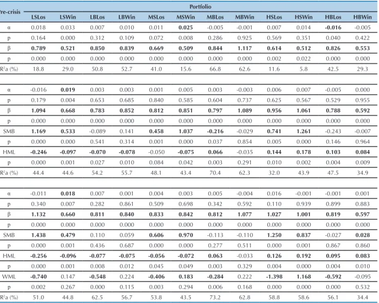
Tables 3 and 4 present the results of the time series regressions for models (1), (2), and (3), in the pre-crisis and post-crisis periods, using the modiied method for portfolio formation. All of the analyses were carried out using the SELIC rate as a risk-free asset and the results obtained were similar. he analyses were also made compiling the portfolios using the method proposed by Fama and French, however there was a gain in the predictive power of the models using the method proposed in this article, which varied from 3% for the CAPM to 61% in the case of the four factor model for the post-crisis period. All of the results are available upon requesting them from the authors.
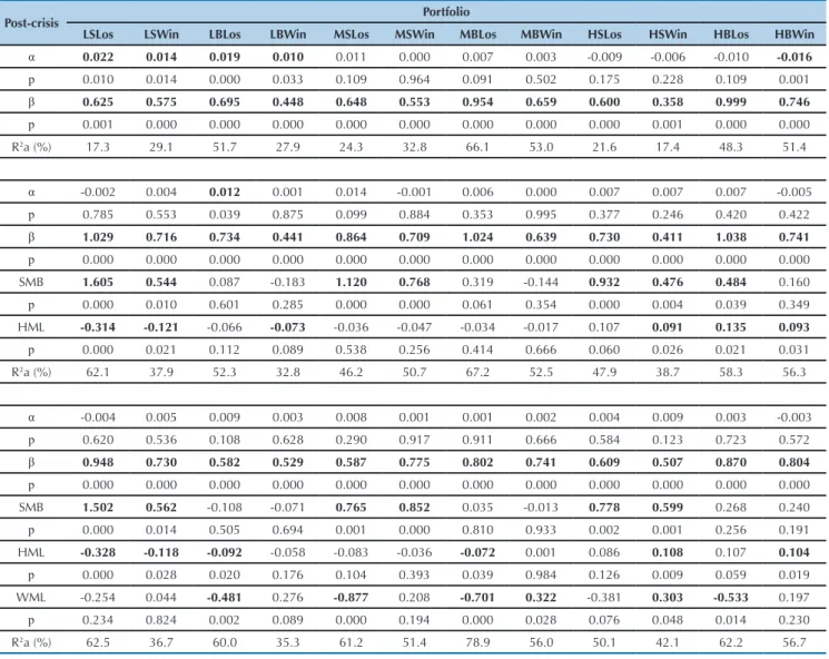
Analyzing the CAPM intercept, it is veriied that for three out of 12 portfolios before the crisis, and ive out of 12 portfolios ater the crisis, this coeicient is diferent from zero, with 95% conidence, which would contradict the CAPM hypotheses, as previously discussed. his indicates that the market risk factor is not enough to capture all of the risk premiums in the Brazilian market. hus, the multifactor models would be better, since for only one portfolio the intercept was statistically relevant to 5% signiicance before
the crisis, and this was the case for none of them ater the crisis, which leads to the conclusion that the multifactor models used managed to capture the anomalies existing in the market. Also according to Table 4, in considering only the market risk factor, the four low BM index portfolios present positive excess returns (α), always to 5% signiicance. his result difers from that indicated by Stattman (1980) and Fama and French (1993), as was mentioned.
In accordance with what was expected, the β coeicient, which measures sensitivity to the market risk factor, presented a positive sign and statistical signiicance to 5% for all of the portfolios and models, that is, even ater considering the other factors. Despite the importance of the market risk factor, it was not enough to capture all of the risk premiums in the Brazilian market, as was mentioned in the previous paragraph.
and winning companies, low BM index, big, and winning companies, medium BM index, big, and winning companies, and high BM index, big and winning companies.
Based on the results from the four factor model, it is important to note that 75% of the portfolios (9 out of 12) descriptively presented β coeicients with a smaller magnitude ater the crisis, which indicates a decrease in sensitivity to the market factor ater the crisis in the Brazilian market. SBM was relevant for around half of the portfolios, both before and ater the crisis, with WML presenting statistical relevance for little more than half of the portfolios
considered in each one of the periods. HML presented statistical relevance for most of the portfolios before the crisis (11 out of 12), and ater the crisis sensitivity to this factor reduced, with only six out of 12 portfolios having coeicients that were statistically signiicant to 5%.
Regressions for the crisis period were also carried out and the results are available upon requesting them from the authors. he main diference was in the reduction in the importance of HML in the crisis and post-crisis periods when compared with the pre-crisis period.
Table 3 - Results from the time series regressions for the CAPM and 3 and 4 factor models in the pre-crisis period, using the
modiied method for forming portfolios
Pre-crisis Portfolio
LSLos LSWin LBLos LBWin MSLos MSWin MBLos MBWin HSLos HSWin HBLos HBWin
α 0.018 0.033 0.007 0.010 0.011 0.025 -0.005 -0.001 0.007 0.014 -0.016 -0.005
p 0.164 0.000 0.312 0.109 0.072 0.008 0.286 0.925 0.569 0.351 0.040 0.422
β 0.789 0.521 0.850 0.839 0.669 0.509 0.844 1.117 0.614 0.512 0.826 0.553
p 0.000 0.000 0.000 0.000 0.000 0.000 0.000 0.000 0.002 0.022 0.000 0.000
R2a (%) 18.8 29.0 50.8 52.7 41.0 15.6 66.8 62.6 11.6 5.8 42.5 29.3
α -0.016 0.019 0.003 0.003 0.001 0.005 0.003 -0.003 0.006 0.007 -0.005 0.000
p 0.179 0.004 0.653 0.685 0.840 0.585 0.604 0.737 0.625 0.567 0.529 0.955
β 1.094 0.668 0.783 0.852 0.812 0.851 0.797 1.089 0.956 1.061 0.788 0.592
p 0.000 0.000 0.000 0.000 0.000 0.000 0.000 0.000 0.000 0.000 0.000 0.000
SMB 1.169 0.533 -0.089 0.141 0.458 1.037 -0.216 -0.029 0.741 1.261 -0.243 -0.007
p 0.000 0.000 0.541 0.314 0.001 0.000 0.037 0.854 0.005 0.000 0.146 0.964
HML -0.246 -0.097 -0.070 -0.078 -0.050 -0.075 0.066 -0.035 0.144 0.178 0.103 0.084
p 0.000 0.001 0.027 0.010 0.084 0.042 0.003 0.291 0.010 0.002 0.004 0.009
R2a (%) 44.4 44.6 54.2 55.7 48.1 43.4 70.4 62.3 32.0 43.9 47.5 34.9
α -0.011 0.018 0.007 0.001 0.004 0.003 0.005 -0.004 0.016 -0.001 -0.001 0.001
p 0.340 0.007 0.282 0.861 0.509 0.698 0.342 0.592 0.110 0.939 0.899 0.883
β 1.132 0.660 0.811 0.840 0.833 0.842 0.812 1.077 1.027 1.001 0.819 0.597
p 0.000 0.000 0.000 0.000 0.000 0.000 0.000 0.000 0.000 0.000 0.000 0.000
SMB 1.438 0.479 0.110 0.059 0.606 0.970 -0.113 -0.110 1.250 0.837 -0.027 0.028
p 0.000 0.001 0.436 0.687 0.000 0.000 0.277 0.511 0.000 0.001 0.867 0.860
HML -0.256 -0.096 -0.077 -0.075 -0.056 -0.072 0.063 -0.033 0.126 0.192 0.095 0.083
p 0.000 0.001 0.008 0.012 0.045 0.049 0.003 0.329 0.004 0.000 0.004 0.010
WML -0.740 0.147 -0.548 0.224 -0.406 0.183 -0.284 0.222 -1.398 1.168 -0.592 -0.095
p 0.002 0.267 0.000 0.115 0.003 0.294 0.006 0.168 0.000 0.000 0.000 0.532
R2a (%) 51.0 44.8 62.5 56.7 53.8 43.5 73.2 62.8 58.8 58.6 56.1 34.4
Note. Models (1), (2), and (3) are separated in this order by the lines in the table. In bold are the coeficients that presented
statistical signiicance to 5%.
Table 4 - Results from the time series regressions for the CAPM and 3 and 4 factor models in the post-crisis period, using the modiied method for forming portfolios
Post-crisis Portfolio
LSLos LSWin LBLos LBWin MSLos MSWin MBLos MBWin HSLos HSWin HBLos HBWin α 0.022 0.014 0.019 0.010 0.011 0.000 0.007 0.003 -0.009 -0.006 -0.010 -0.016
p 0.010 0.014 0.000 0.033 0.109 0.964 0.091 0.502 0.175 0.228 0.109 0.001
β 0.625 0.575 0.695 0.448 0.648 0.553 0.954 0.659 0.600 0.358 0.999 0.746
p 0.001 0.000 0.000 0.000 0.000 0.000 0.000 0.000 0.000 0.001 0.000 0.000
R2a (%) 17.3 29.1 51.7 27.9 24.3 32.8 66.1 53.0 21.6 17.4 48.3 51.4
α -0.002 0.004 0.012 0.001 0.014 -0.001 0.006 0.000 0.007 0.007 0.007 -0.005
p 0.785 0.553 0.039 0.875 0.099 0.884 0.353 0.995 0.377 0.246 0.420 0.422
β 1.029 0.716 0.734 0.441 0.864 0.709 1.024 0.639 0.730 0.411 1.038 0.741
p 0.000 0.000 0.000 0.000 0.000 0.000 0.000 0.000 0.000 0.000 0.000 0.000
SMB 1.605 0.544 0.087 -0.183 1.120 0.768 0.319 -0.144 0.932 0.476 0.484 0.160
p 0.000 0.010 0.601 0.285 0.000 0.000 0.061 0.354 0.000 0.004 0.039 0.349
HML -0.314 -0.121 -0.066 -0.073 -0.036 -0.047 -0.034 -0.017 0.107 0.091 0.135 0.093
p 0.000 0.021 0.112 0.089 0.538 0.256 0.414 0.666 0.060 0.026 0.021 0.031
R2a (%) 62.1 37.9 52.3 32.8 46.2 50.7 67.2 52.5 47.9 38.7 58.3 56.3
α -0.004 0.005 0.009 0.003 0.008 0.001 0.001 0.002 0.004 0.009 0.003 -0.003
p 0.620 0.536 0.108 0.628 0.290 0.917 0.911 0.666 0.584 0.123 0.723 0.572
β 0.948 0.730 0.582 0.529 0.587 0.775 0.802 0.741 0.609 0.507 0.870 0.804
p 0.000 0.000 0.000 0.000 0.000 0.000 0.000 0.000 0.000 0.000 0.000 0.000
SMB 1.502 0.562 -0.108 -0.071 0.765 0.852 0.035 -0.013 0.778 0.599 0.268 0.240
p 0.000 0.014 0.505 0.694 0.001 0.000 0.810 0.933 0.002 0.001 0.256 0.191
HML -0.328 -0.118 -0.092 -0.058 -0.083 -0.036 -0.072 0.001 0.086 0.108 0.107 0.104
p 0.000 0.028 0.020 0.176 0.104 0.393 0.039 0.984 0.126 0.009 0.059 0.019
WML -0.254 0.044 -0.481 0.276 -0.877 0.208 -0.701 0.322 -0.381 0.303 -0.533 0.197
p 0.234 0.824 0.002 0.089 0.000 0.194 0.000 0.028 0.076 0.048 0.014 0.230
R2a (%) 62.5 36.7 60.0 35.3 61.2 51.4 78.9 56.0 50.1 42.1 62.2 56.7
Note. Models (1), (2), and (3) are separated in this order by the lines in the table. In bold are the coeficients that presented
statistical signiicance to 5%.
Source: Elaborated by the authors.
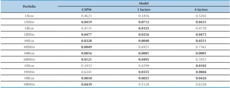
he Chow test (Wooldridge, 2014), presented in Table 5, conirms the existence of diferences between the results from all of the models estimated before the crisis (Table 3) and ater the crisis (Table 4), indicating the existence of a structural break in the 2008 crisis. Using a 10% level
Table 5 - p value results from the Chow test for comparing the models estimated in the pre-crisis and post-crisis periods
Portfolio Model
CAPM 3 factors 4 factors
LSLos 0.4623 0.3416 0.5265
LSWin 0.0459 0.0712 0.0431
LBLos 0.4131 0.0325 0.4739
LBWin 0.0477 0.0256 0.0475
MSLos 0.0328 0.0040 0.0251
MSWin 0.0049 0.6921 0.7361
MBLos 0.0016 0.0001 0.0001
MBWin 0.0121 0.0495 0.3953
HSLos 0.3933 0.6599 0.0102
HSWin 0.6341 0.0355 0.0084
HBLos 0.0850 0.0025 0.0426
HBWin 0.0439 0.5128 0.6328
Note. In bold are the coeficients that presented statistical signiicance to 10%.
Source: Elaborated by the authors.
Ater the time series regressions, the estimated coeicients were used in a second, cross-sectional regression, in order to obtain the predicted return for each one of the 12 portfolios in accordance with what was expected by each one of the three models analyzed. Table 6 presents two diferent metrics (RMSE and MAPE) for the prediction error in the cross-sectional regression, with for each statistic used, the lower the value, the better the prediction quality. Analysis of the table indicates that, generally, the four factor model presented the best prediction results, which was expected due to it containing a greater number of variables. However, in some sub-periods this superiority was marginal. If parsimony is a criterion for choosing the model, the three factor one can be taken into consideration. Other information that warrants
attention is the signiicant improvement in the predictiveness of the three and four factor models for the post-crisis period, which can be credited to the lack of “contamination” in the data caused by the crisis.
he fourth and ith columns in Table 6 present the gain in prediction quality by using the multifactor models instead of the CAPM, in which we observe a signiicant improvement in predictability. As is to be expected, the model with the greatest number of factors presents the best prediction results. However, the gain is marginal in the pre-crisis and crisis periods. For the post-crisis period, an improvement of more than 40% is noted by using the four factor model instead of the three factor one.
Table 6 -Prediction quality measures of the CAPM (capital asset pricing model) and the three and four factor models using a
constant for the pre-crisis, crisis, post-crisis, and total periods, using the modiied method for forming portfolios
Period Model
Prediction quality gain in relation to the CAPM (%)
CAPM Three factors Four factors Three factors Four factors
RMSE
Pre-crisis 0.0112 0.0063 0.0059 44.19* 47.93*
Crisis 0.0157 0.0079 0.0078 49.57* 49.64*
Post-crisis 0.0104 0.0035 0.0021 63.33** 80.03**
Total 0.0102 0.0047 0.0046 53.84** 54.03**
MAPE
Pre-crisis 169.57 72.17 65.02 57.44 61.66
Crisis 116.63 55.11 52.66 52.75 54.85
Post-crisis 91.47 33.43 27.98 63.45** 69.41**
Total 98.50 48.96 48.32 50.29* 50.94*
Note. In bold are the lowest measures between the models used.
MAPE = mean absolute percentage error; RMSE = root mean square error.
6 CONCLUSION
his study analyzed the single-factor asset pricing model and the multifactor ones with three and four factors for the Brazilian equities market in the period from 2002 to 2013. Risk premiums, time series regressions, and the predictive power of the models were analyzed in the complete period and dividing the period using the 2008 crisis.
We found a market risk premium consistent with the theory, however with a lower value than that of other studies of the Brazilian market, which we considered normal due to the period evaluated in this paper considering the 2008 crisis. he premium found regarding SMB was positive, in accordance with what was expected, however diferent from studies for the Brazilian market, such as those from Málaga and Securato (2004) and from Mussa, Famá, and Santos (2012). he premium regarding HML presented a diferent sign from expected, while WML was statistically insigniicant. hese premiums are anomalies by nature. In the case of SMB, smaller companies tend to generate an abnormally higher return than larger companies, which was conirmed in our paper. With regards to the HML factor, we also expected a positive sign, as in the indings from Fama and french (1993), but we may not have managed to conirm previous studies due to “errors in the variables” that may be present in less liquid shares and due to not having true growth shares in Brazil, as is the case in the United States of America, primarily characterized by technology companies. In the case of WML, we did not obtain signiicance, possibly because of the diferent behaviors from those found by Fama and French (1993) in the case of losing shares, in which the momentum efect appears to have an opposite efect.
he results from the time series regressions reveal that the market risk factor is the most important for explaining portfolio returns, however it is not the only one with
statistical signiicance. For most of the portfolios, the three and four factor models obtain a signiicant improvement in the adjusted R2, conirming the existence of anomalies in the Brazilian equities market, as was veriied in other studies (Argolo et al. 2012; Málaga & Securato, 2004; Mussa, Famá & Santos, 2012), in which the factors that represent statistically relevant anomalies for most of the portfolios were HML and WML.
Future studies are necessary in which portfolio assets are separated using diferent criteria, such as using the asset beta, as suggested by Lewellen, Nagel, and Shanken (2010). By analyzing the results from the various sub-periods it is observed that the variations in the estimates for the beta of the same portfolio are large, reaching up to 100%, which may indicate that the beta must vary over time, as in the study from Bollerslev, Engle, and Wooldridge (1988) and Bortoluzzo, Toloi, and Morettin (2010), for the autoregressive model of conditional duration. Our analysis indicated greater betas during the crisis, indicating that systematic risk gains importance in the crisis period.
Analysis of the predictive power of the models indicated a signiicant gain in predictive quality by using the multifactor model instead of the single factor one. For the total sample period, the gain was an approximately 54% reduction in RSME. Moreover, we observed that for the most recent sub-period, the inclusion of WML into the three factor model from Fama and French generated an expressive improvement in prediction quality. Finally, we observed a signiicant improvement in the predictability of the four factor model for the post-crisis period, contradicting common sense that the use of a longer period in the sample generates better results.
References
Araújo, E. A. T., Oliveira, V. C., & Silva, W. A. C. (2012). CAPM em estudos brasileiros: uma análise da pesquisa. Revista de Contabilidade e Organizações, 15(6), 95-122.
Argolo, E. F. B., Leal, R. P. C., & Almeida, V. S. (2012). O modelo de Fama e French é aplicável no Brasil? Relatório COPPEAD, 402.
Banz, R. W. (1981) he relationship between return and market value of common stocks. Journal of Financial Economics, 9, 3-18.
Black, F., Jensen, M. C., & Scholes, M. (1972). he capital asset pricing model: some empirical tests. In M. C. Jensen (Ed.), Studies in the
theory of capital markets (pp. 79-121). New York, NY: Praeger
Publishers Inc.
Bodurtha Jr., J. N., & Mark, N. C. (1991). Testing the CAPM with time-varying risks and returns. he Journal of Finance, 46(4), 1485-1505. Bollerslev, T., Engle, R. F., & Wooldridge, J. M. (1988). A capital asset
pricing model with time-varying covariances. Journal of Political Economy, 96(1), 116-131.
Bortoluzzo, A. B., Minardi, A. M. A. F., & Passos, B. C. (2014). Analysis of multi-scale systemic risk in Brazil’s inancial market. Revista de
Administração (FEA-USP), 49, 240-250.
Bortoluzzo, A. B., Toloi, C. M. C., & Morettin, P. A. (2010). Time-varying autoregressive conditional duration model. Journal of Applied Statistics, 37, 847-864.
Carhart, M. M. (1997). On persistence in mutual fund performance. he Journal of Finance, 52, 57-82.
Fama, E. F., & French, K. R. (1993). Common risk factors in the returns on stocks and bonds. Journal of Financial Economics, 33, 3-56. Fama, E. F., & MacBeth, J. D. (1973). Risk, return, and equilibrium:
Empirical tests. he Journal of Political Economy, 81(3), 607-636 Garcia, R., & Bonomo, M. (2001). Tests of conditional asset pricing
models in the Brazilian stock market. Journal of International Money and Finance, 20(1), 71-90.
Garcia, R., & Ghysels, E. (1998). Structural change and asset pricing in emerging markets. Journal of International Money and Finance,
Jegadeesh, N., & Titman, S. (1993). Returns to buying winners and selling losers: implications for stock market eiciency. Journal of Finance,
48, 65-91.
Jegadeesh, N., & Titman, S. (2001). Proitability of momentum strategies: an evaluation of alternative explanations. Journal of Finance, 56(2), 699-720.
Lewellen, J., & Nagel, S. (2006). he conditional CAPM does not explain asset-pricing anomalies. Journal of Financial Economics, 82, 289-314. Lewellen, J., Nagel, S., & Shanken, J. (2010). A skeptical appraisal of asset
pricing tests. Journal of Financial Economics, 96, 175-194. Lintner, J. (1965). he valuation of risk assets and the selection of risky
investments in stock portfolios and capital budgets. Review of Economics and Statistics, 47(1), 13-37.
Machado, M. A. V., & Medeiros, O. R. (2011). Modelos de preciicação de ativos e o efeito liquidez: evidências empíricas no mercado acionário brasileiro. Revista Brasileira de Finanças, 9, 383-412.
Machado, O. P, Bortoluzzo, A. B., Martins, S. R, & Sanvicente, A. Z. (2013). Inter-temporal CAPM: an empirical test with Brazilian market data. Brazilian Finance Review, 11, 149-180.
Málaga, F. K., & Securato, J. R. (2004). Aplicação do modelo de três fatores de Fama e French no mercado acionário brasileiro: um estudo empírico no período 1995-2003. Anaisdo Encontro Anual da Associação Nacional de Programas de Pós-Graduação em Administração, Curitiba, PR, Brasil, 28.
Mussa, A., Famá, R., & Santos, J. O. (2012). A adição do fator de risco momento ao modelo de preciicação de ativos dos três fatores de Fama & French aplicado ao mercado acionário brasileiro. REGE,
19(3), 431-447.
Mussa, A., Rogers, P., & Securato, J. R. (2009). Modelos de retornos esperados no mercado brasileiro: testes empíricos utilizando metodologia preditiva. Revista de Ciências da Administração, 11(23), 192-216.
Noda, R. F., Martelanc, R., & Kayo, E. K. (2015). he earnings/price risk factor in capital asset pricing models. Revista Contabilidade & Finanças, 27(70), 67-79.
Phillips, P. C. B., & Yu, J. (2011). Dating the timeline of inancial bubbles during the subprime crisis. Quantitative Economics, 2, 455-491. Rayes, A. C. R. W., Araújo, G. S., & Barbedo, C. H. S. (2012). O modelo
de 3 fatores de Fama e French ainda explica os retornos no mercado acionário brasileiro? Revista Alcance, 19(1), 52-61.
Rogers, P., & Securato, J. R. (2009). Estudo comparativo no mercado brasileiro do capital asset pricing model (CAPM). RAC Eletrônica,
3(1), 159-179.
Roll, R. (1977). A critique of the asset pricing theory’s tests. Part 1. On past and potential testability of the theory. Journal of Financial Economics, 4, 129-176.
Sandoval Jr., L., Bortoluzzo, A. B., & Venezuela, M. K. (2014). Not all that glitters is RMT in the forecasting of risk of portfolios in the Brazilian stock market. Physica A, 410, 94-109.
Sanvicente, A. Z. (2014). O mercado de ações no Brasil antes do índice Bovespa. Revista Brasileira de Finanças, 12(1), 1-12.
Sharpe, W. F. (1964). Capital assets prices: a theory of market equilibrium under conditions of risk. Journal of Finance, 19(3), 425-442. Silva, A. R. (2016). Biotools: tools for biometry and applied statistics in
agricultural science. R package, version 3. 0. Retrieved from https:// cran.rstudio.com/web/packages/biotools/biotools.pdf.
Silva, W. A. C., Pinto, E. A., Melo, A. O., & Camargos, M. A. (2009). Análise comparativa entre o CAPM e o C-CAPM na preciicação de índices acionários: evidências de mudanças nos coeicientes estimados de 2005 a 2008. Anais do IX Encontro Brasileiro de Finanças, São Paulo, SP, Brasil,
Stattman, D. (1980). Book values and stock returns. he Chicago MBA: A Journal of Selected Papers, 4, 25-45.
Tambosi Filho, E., da Costa Jr., N. C. A., & Rossetto, J. R. (2006). Testando o CAPM condicional nos mercados brasileiro e norte-americano.
Revista de Administração Contemporânea, 10(4), 53-168.
Vayanos, D., & Woolley, P. (2013). An institutional theory of momentum and reversal. he Review of Financial Studies, 26(5), 1087-1145. Wooldridge, J. M. (2014). Introdução à econometria: uma abordagem
moderna. São Paulo, SP: Cengage Learning.
Correspondence address:
Adriana Bruscato Bortoluzzo
Insper, Departamento de Ciências Econômicas Rua Quatá, 300 – CEP: 04546-042