Nat. Hazards Earth Syst. Sci., 16, 2729–2745, 2016 www.nat-hazards-earth-syst-sci.net/16/2729/2016/ doi:10.5194/nhess-16-2729-2016
© Author(s) 2016. CC Attribution 3.0 License.
The propagation of inventory-based positional errors into statistical
landslide susceptibility models
Stefan Steger1, Alexander Brenning2, Rainer Bell1, and Thomas Glade1
1Department of Geography and Regional Research, University of Vienna, Universitätsstraße 7, 1010 Vienna, Austria 2Department of Geography, Friedrich Schiller University Jena, Loebdergraben 32, 07743 Jena, Germany
Correspondence to:Stefan Steger ([email protected])
Received: 12 September 2016 – Published in Nat. Hazards Earth Syst. Sci. Discuss.: 14 September 2016 Revised: 29 November 2016 – Accepted: 1 December 2016 – Published: 16 December 2016
Abstract.There is unanimous agreement that a precise spa-tial representation of past landslide occurrences is a prerequi-site to produce high quality statistical landslide susceptibility models. Even though perfectly accurate landslide inventories rarely exist, investigations of how landslide inventory-based errors propagate into subsequent statistical landslide suscep-tibility models are scarce.
The main objective of this research was to systematically examine whether and how inventory-based positional inaccu-racies of different magnitudes influence modelled relation-ships, validation results, variable importance and the visual appearance of landslide susceptibility maps. The study was conducted for a landslide-prone site located in the districts of Amstetten and Waidhofen an der Ybbs, eastern Austria, where an earth-slide point inventory was available.
The methodological approach comprised an artificial in-troduction of inventory-based positional errors into the present landslide data set and an in-depth evaluation of sub-sequent modelling results. Positional errors were introduced by artificially changing the original landslide position by a mean distance of 5, 10, 20, 50 and 120 m. The resulting dif-ferently precise response variables were separately used to train logistic regression models. Odds ratios of predictor vari-ables provided insights into modelled relationships. Cross-validation and spatial cross-Cross-validation enabled an assessment of predictive performances and permutation-based variable importance. All analyses were additionally carried out with synthetically generated data sets to further verify the findings under rather controlled conditions.
The results revealed that an increasing positional inventory-based error was generally related to increasing distortions of modelling and validation results. However,
the findings also highlighted that interdependencies between inventory-based spatial inaccuracies and statistical landslide susceptibility models are complex. The systematic compar-isons of 12 models provided valuable evidence that the re-spective error-propagation was not only determined by the degree of positional inaccuracy inherent in the landslide data, but also by the spatial representation of landslides and the environment, landslide magnitude, the characteristics of the study area, the selected classification method and an inter-play of predictors within multiple variable models. Based on the results, we deduced that a direct propagation of minor to moderate inventory-based positional errors into modelling results can be partly counteracted by adapting the modelling design (e.g. generalization of input data, opting for strongly generalizing classifiers). Since positional errors within land-slide inventories are common and subsequent modelling and validation results are likely to be distorted, the potential ex-istence of inventory-based positional inaccuracies should al-ways be considered when assessing landslide susceptibility by means of empirical models.
1 Introduction
For large regions or areas where detailed geotechnical in-formation is missing, statistically based approaches are most commonly applied to generate landslide susceptibility maps (Cascini, 2008; Corominas et al., 2013; Van Westen et al., 2008). The underlying concept is based on a modified uni-formitarian principle (Hutton, 1788) by assuming that future landslides evolve more likely under those environmental con-ditions that led to past slope movements (Brabb, 1984; Er-mini et al., 2005; Fabbri et al., 2003; Fell et al., 2008; Glade et al., 2005).
In practice, this idea is operationalized by fitting a binary classification model to a data set containing spatial infor-mation on the presence and absence of past landslides (re-sponse) and a number of associated static preparatory envi-ronmental factors (predictors; e.g. slope, lithology). The re-sulting classification rule allows to identify conditions that were likely to promote past slope movements and conditions that favoured slope stability. When the constructed model is considered to appropriately describe the underlying relation-ship, a likelihood of landslide occurrence can be assigned to all spatial units containing information on these environmen-tal conditions. Thus, a specific location shows a high land-slide susceptibility whenever the respective environmental setting is similar to the conditions observed for past land-slide occurrences (Ermini et al., 2005; Goetz et al., 2015b; Petschko et al., 2014a; Van Den Eeckhaut et al., 2006).
The quality and applicability of a landslide susceptibility map is regularly inferred from predictive performance es-timates which compare the predicted susceptibility pattern with an independent data set that is supposed to mimic future landslide locations (Beguería, 2006; Brenning, 2005; Chung and Fabbri, 2003; Frattini et al., 2010; Remondo et al., 2003). An issue found by many authors is that the quality of the presented landslide susceptibility map is directly related to the quality of the input data used to construct the underly-ing model (Cascini, 2008; Corominas et al., 2013; Fressard et al., 2014; Guzzetti et al., 2006; Van Westen et al., 2008). In this context, an accurate representation of past landslide activities (landslide inventory) is regularly considered as a crucial component to produce reliable results (Ardizzone et al., 2002; Fressard et al., 2014; Galli et al., 2008; Guzzetti et al., 2012; Harp et al., 2011; Hussin et al., 2016; Steger et al., 2015, 2016). However, perfect landslide inventories are known to be rarely available (Malamud et al., 2004; Petschko et al., 2016). Several studies emphasize that the positional accuracy of a landslide inventory can vary greatly and is in-fluenced by the type (e.g. aerial photograph, shaded-relief image) and quality (e.g. spatial resolution) of available base maps, the type and sizes of mapped landslides, human fac-tors (e.g. accuracy of public reports, covered time period) and the processing of analogue information sources (e.g. digitiza-tion) (Ardizzone et al., 2002; Harp et al., 2011; Petschko et al., 2016; Santangelo et al., 2015).
A number of authors compared landslide susceptibility models generated from different inventories (e.g. Ardizzone
et al., 2002; Fressard et al., 2014; Galli et al., 2008; Steger et al., 2015, 2016; Zêzere et al., 2009). However, differences between the respective landslide inventories could only be approximated in relative terms due to a variety of underlying data sources and an unavailability of quantitative information on the specific positional errors. Thus, specific statements on how a particular positional error may propagate into the final models and maps could not be made.
This study aims to shed more light on the impact of po-sitionally erroneous landslide inventories on the results of statistical landslide susceptibility models by artificially con-trolling for the extent of positional inaccuracy inherent in the respective data set. The main objective was to systematically examine the influence of positionally inaccurate landslide in-ventories on modelled relationships, validation results and the appearance of landslide susceptibility maps. All analy-ses were also conducted with synthetically generated data to further validate the results under controlled conditions.
2 Study area
The study site extends over 100 km2(20 km×5 km) and is located in the eastern part of Austria (Fig. 1a). The area be-longs to the Lower Austrian districts Amstetten and Waid-hofen an der Ybbs. Altitudes range from less than 350 m a.s.l. in the northern valley bottoms to 790 m a.s.l. at the southern hilltops. The landslide-prone area (5.9 landslides/km2) can be characterized as a hilly undulating landscape with an av-erage slope gradient of 11◦(Fig. 1b).
The morphological and lithological condition of the study site plays a major role for the propensity of the respective slopes to fail. The major part of the area (81 km2) relates to alternating sediment sequences of the Rheno-Danubian Fly-sch Zone (Fig. 1c). Several publications emphasize that the high density of shallow landsliding within the Flysch is re-lated to the widespread presence of deeply weathered soils consisting of silts and clayey material (Petschko et al., 2016; Schwenk, 1992; Wessely et al., 2006). A minor portion of the terrain (3 km2) can be assigned to clastic sediments of the Molasse Zone. The Molasse lies along the northern side of the Eastern Alps and is regularly associated with several me-tre thick clayey and marly soils which tend to be susceptible to landsliding, even at lower slope gradients (Wessely et al., 2006; Petschko et al., 2016). Quaternary sediments (16 km2) that relate to alluvial deposits and fluvial terraces dominantly cover the valley floors of the area. Landslide density is low within this area, mainly due to its prevalent flat topography (compare Fig. 1b with Fig. 1c).
S. Steger et al.: The propagation of inventory-based positional errors 2731
Figure 1. Location of the study area within Austria (a), shaded relief image of the area with an overlaid slope angle map and spatial
distribution of landslide scarps(b). The shaded relief images (top right) show typical landslides of the study area and the corresponding mapping location. Lithological units are given in(c)while slope orientation is represented as northness(d)and eastness(e). The photograph
(source: K. Gokesch) in(f)relates to the northern part of Waidhofen an der Ybbs and shows a characteristic shallow landslide of the Flysch Zone.
friction and increase in water-related loading are considered to be the main driving forces along a regularly distinct slid-ing plane. However, also human interventions were observed to be an increasingly important landslide influencing factor (Schwenk, 1992; Wessely et al., 2006). The southern hilly areas are for the most parts used for intensive cattle farm-ing (e.g. pastures) or covered by forests while arable land is prevalent in the northern lying flat lowlands (Eder et al., 2011). The area lies in a transitional climate zone (oceanic influences from the west and continental influences from the east) with mean annual precipitation rates around 1000 mm (Skoda and Lorenz, 2007).
The majority of landslides in the area are relatively small and shallow. Petschko et al. (2016) investigated landslide sizes for the districts Amstetten, Waidhofen an der Ybbs and Baden and found a median size of landslides of the slide-type movement of 787 m2for the Rheno-Danubian Flysch Zone, 1189 m2 for the Molasse Zone and 1260 m2for Quaternary sediments. Based on an analysis of landslide archive entries (i.e. Building Ground Registry), Bell et al. (2014a) estimated a median landslide depth of 1.7 m (mean 2.2 m) for 142 land-slides recorded for the district Waidhofen an der Ybbs.
3 Data
3.1 Landslide inventory
3.2 Predictor variables
The number and type of predictors used within statistical landslide susceptibility analyses varies greatly depending on the scope of the study, the type of the investigated landslides, the characteristics of the area and data availability (Guzzetti et al., 1999; Van Westen et al., 2008). To enhance trace-ability of modelling results, we opted to include only few but widely used predictors within the analyses. All models were generated with a predictor set consisting of a lithol-ogy layer (Fig. 1c) and three topographic variables, namely slope (Fig. 1b) and two variables representing slope orienta-tion (Fig. 1d, e).
The inclination of a slope is directly related to shear stresses and therefore almost always used as a predictor within statistical landslide susceptibility modelling. Slope as-pect is regularly introduced as a proxy for a varying degree of insolation and evapotranspiration influencing moisture and weathering conditions or, in some cases, as a representative for the dipping of geologic structures (Gorsevski et al., 2006; Van Westen et al., 2008). The two slope azimuth predictors were directly derived from a resampled (10 m×10 m) ALS-based DTM. Classification of the continuously scaled aspect layer (originally ranging from 0 to 360◦) was avoided by
cal-culating its cosine (representing the degree of north exposed-ness) and sine (east exposedexposed-ness) (Brenning, 2009, 2012a). This transformation ensured that the applied linear models treated similarly oriented slopes (e.g. 1◦vs. 360◦) similarly.
At regional scales, the parent material of the soils is usually represented by lithological maps (Gorsevski et al., 2006; Van Westen et al., 2008). This information was obtained from a digital geological map of Lower Austria (GK200) available at a scale of 1 : 200 000 and resampled to the modelling res-olution of 10 m×10 m.
We decided to exclude land cover from the analysis for two reasons. Firstly, the available recent land cover data do not necessarily correspond to the land cover present at the time of landslide occurrence, due to constantly ongoing land use changes and the fact that landslide age is expected to vary substantially within the present inventory (Petschko et al., 2014b; Van Westen et al., 2008). Secondly, an omission of land cover as a predictor was expected to reduce the chances that the suspected land cover related-bias (e.g. overrepresen-tation of landslides in forested areas; see Bell et al., 2012; Petschko et al., 2016) is directly propagated into the final re-sults (see Steger et al., 2016). However, land cover was intro-duced as a predictor within the synthetic data set, because the respective landslide data set was not defined to be affected by a systematic error, while land cover was specified to be static in time (see Sect. 4.6).
4 Methods
In this study we aimed to analyse all data in a tangible and traceable way. Therefore, we avoided using less interpretable classifiers or a high number of predictors. For classification we opted for the well-established logistic generalized lin-ear model, also known as logistic regression (see Sect. 4.2), while we included only a small number of frequently ap-plied predictors (see Sect. 3.2). The general methodologi-cal framework consisted of an artificial introduction of po-sitional inaccuracies into the present landslide inventory (see Sect. 4.1) and a subsequent in-depth evaluation of modelling results. The final response variable included within each model was based on an equal number of landslide presence-observations (landslide inventory) and randomly sampled absence-observations (1:1 sampling) (Goetz et al., 2015a; Heckmann et al., 2014). All analyses were additionally per-formed with synthetic data in order to further verify the ob-servations under rather controlled conditions (see Sect. 4.6). 4.1 Artificial introduction of positional errors into the
landslide inventory
Inventory-based positional errors were introduced by artifi-cially changing the original landslide scarp position accord-ing to a normal distribution in a random direction (Fig. 2). The mean distance to the original position was specified as 5, 10, 20, 50 and 120 m (Fig. 2c). Smaller positional inaccu-racies (e.g. 5 or 10 m) may be present when digitizing land-slide inventories mapped through interpretation of aerial pho-tographs (Santangelo et al., 2015) while the highest value (120 m) was defined according to an analysis made for the Flysch Zone. Within this analysis, 65 of the 681 analysed landslide database entries of the Building Ground Registry (more information refer to Schwenk, 1992 and Steger et al., 2016) contained a quantitative estimate on the positional ac-curacy of the respective landslide point location. The derived mean positional error of 120 m (standard deviation of 84 m) was directly adopted to specify the inaccuracy of the most erroneous inventory.
4.2 Logistic regression and odds ratios
S. Steger et al.: The propagation of inventory-based positional errors 2733
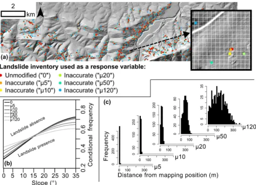
Figure 2.Overview of the simulated positional inaccuracy of the inventory for the study area (real data). The excerpt in(a)shows an example
of an original mapping position of a landslide scarp (red dot) and corresponding simulated positional inaccuracies (the white grid corresponds to the modelling resolution of 10 m). The conditional frequency plot in(b)shows that a decreasing positional accuracy of the inventory led to
the effect that landslides were more likely located on flatter slopes. The histograms in(c)(bin width 10 m) depict the frequency of landslides
(n=591) in relation to the distance from the original mapping position for the respective simulated positional inaccuracy.
occurringP (Y=1)was predicted by:
logit(P (Y=1))=β0+β1X1+. . .+βpXp (1) in which,β0represents the intercept andβ1. . .βpthe regres-sion coefficients of predictorsX1. . .Xp. The associations be-tween predictors and the response within multiple variable regression models can be expressed as odds ratios (OR). In contrast to an interpretation of probabilities, OR allow to ex-press this relation with a single number while accounting for the influence of other predictors (Brenning et al., 2015; Hos-mer and Lemeshow, 2000). For instance, OR estimated for the predictor lithology display the estimated chances that a certain lithological unit is affected by landsliding while ac-counting for the possible confounding effect of slope angle (Steger et al., 2016).
The odds of an event occurring (in this case a landslide) are defined as the probability of this event occurringP (Y=1), divided by the probability that this event is not occurring P (Y=0). The ratio between the odds after a one-unit in-crease in the predictorXpand the original odds is referred to as odds ratio:
OR Xp=Odds Xp +1 Odds Xp
=Odds after a one unit increase in the predictor
Original odds (2)
For logistic regression based models, OR can be directly derived from exponentiated regression coefficients (β1. . .βp). OR of > 1 point to a positive relation between a continu-ously scaled predictor and landslide occurrence while ORs of < 1 express a negative association. Within this study, OR ob-tained for all continuously scaled predictors were estimated for “meaningful” increments (Brenning, 2012a; Brenning et al., 2015; Hosmer and Lemeshow, 2000). For example, ORs presented for the predictor slope angle refer to the changes in the odds for a slope angle increase of 10◦(X
p+10). OR estimated for categorically scaled predictors have to be inter-preted in relation to a specified reference level.
4.3 Comparison with reference models
have little effect in all cases where the estimated OR and the susceptibility maps were similar to their references.
4.4 Assessment of the predictive performance
The prediction skills of the models were estimated by cal-culating the AUROC by applying two partitioning tech-niques, implemented in the R package “sperrorest” (Bren-ning, 2012b), namelyk-fold cross validation (CV) andk-fold spatial cross validation (SCV). In contrast to single hold-out validation, CV and SCV are not based on one single split of the training and test sample (e.g. 80 % for calibration and 20 % for validation), but on a repeated partitioning of the original sample intoksubsamples. In each iteration, a perfor-mance measure (e.g. AUROC) is estimated for one of thek subsamples, while the remaining (k−1) subsamples are com-bined into a training set that is used to calibrate the model. Thus, validation results that are based on CV and SCV are not dependent on one specific sample split. In fact, CV as well as SCV allow that all available data can be used to val-idate and to calibrate the final models. CV is based on a repeated non-spatial random splitting, whereas SCV is per-formed spatially and consists of a repeated spatial partition-ing of the trainpartition-ing sample and test sample (Brennpartition-ing, 2012b; Ruß and Brenning, 2010). In this study, the predictive per-formance of all models was estimated by repeating CV and SCV 50 times with 10 folds per repetition. More specifically, within each of the 50 repetitions, each observation of the re-sponse variable was applied nine times to calibrate the model and once to test the predictive performance. The presented AUROC values refer to the median of these 500 estimates. Previous studies emphasized the suitability of CV and SCV in the context of landslide susceptibility modelling (Goetz et al., 2015a; Petschko et al., 2014a; Steger et al., 2016).
Furthermore, an additional validation strategy was applied in order to quantitatively evaluate and compare the ability of all models to “predict” landslide presences and landslide absences of the unmodified response variable. For this pur-pose, the AUROC was used to compare the predictions of each model with the unmodified landslide inventory (i.e. un-affected by an artificially introduced positional error). This metric relates to the goodness of model fit, whenever the re-spective models were calibrated with an unmodified data set. 4.5 Estimation of predictor importance
Permutation-based variable importance assessments assume that the importance of a specific predictor is directly related to the decrease in classification accuracy or predictive perfor-mance after randomly reordering (i.e. permuting) the values of this predictor (Strobl et al., 2007). In landslide suscepti-bility modelling, permutation-based variable importance was previously applied by Goetz et al. (2015a).
In this study, a predictor importance evaluation was con-ducted to assess whether and how the apparent importance
of a specific predictor changes when the positional accuracy of the inventory changes. Thus, the AUROC decrease of each predictor was assessed on non-spatial (CV) and spatial cross-validation partitions (SCV) using the R package “sperrorest” (Brenning, 2012b; Ruß and Brenning, 2010). Herewith, each predictor was permuted 50 times within each fold leading to a total number of 25 000 permutations per predictor (50 repe-titions times 10 folds times 50 permutations) within each par-titioning technique (CV and SCV) for each of the 12 models. 4.6 Generation of synthetic data
None of the susceptibility models generated for the present study area can be considered to reflect a true and unbiased re-lation between landslides and environmental conditions, es-pecially due to the unavailability of perfect and accurate spa-tial information (i.e. landslide data and predictors) and the in-herent subjectivity involved during model construction (e.g. predictor and classifier selection). Thus, the conducted com-parison of a reference model with models generated with er-roneous inventories may only provide an indication of the effect of inventory-based inaccuracies on modelling results. Thus, all analyses were additionally performed with synthet-ically generated data. This procedure allowed us to define a “true” association between landslides and their predispos-ing factors while further controllpredispos-ing for environmental condi-tions (e.g. spatial distribution and interrelacondi-tions between pre-dictors) and model specific parameters (e.g. sample size).
The preparation of synthetic data consisted of three major steps: (i) designing the environmental conditions of the study area (=predictors), (ii) specifying a “true” relation between landslides and predictors and (iii) simulating a landslide dis-tribution within the study area according to the predefined “true” relation.
The areal extent of the synthetic study site (20 km×5 km) was adopted from the Lower Austrian study area while a to-pographically diverse terrain was generated by generalizing an already available DTM (see 3-D image in Fig. 3a). The topographic predictors slope (Fig. 3a) and both aspect layers (Fig. 3b, c) were directly derived from this smoothed DTM, which was expected to be unaffected by local data noise and to represent undisturbed pre-failure conditions (see Van Den Eeckhaut et al., 2006). Lithology and land cover layers were generated by systematically intersecting and reclassi-fying randomly generated raster files produced at different spatial scales. The resulting noisy appearing grid files were smoothed and resampled (Fig. 3d, e).
flat-S. Steger et al.: The propagation of inventory-based positional errors 2735
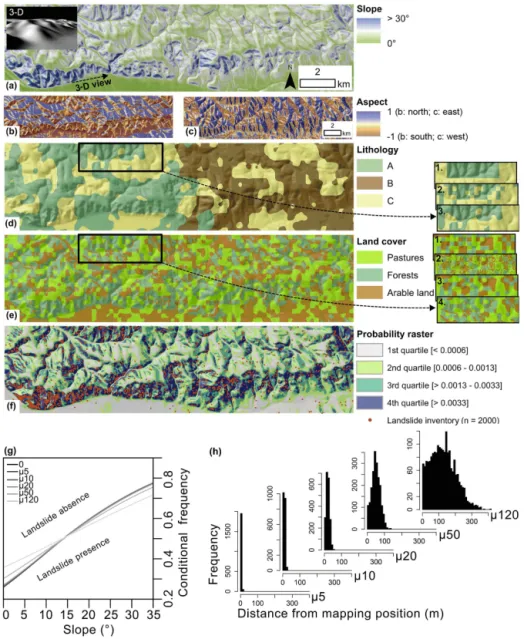
Figure 3.Spatial representation of the synthetically generated data set. Topographic parameters(a, b, c); Lithological and land cover units(d, e)with excerpts depicting the generation of this data sets (1: initial random raster; 2: intersection with a random raster produced at a higher spatial resolution; 3: moving window-based smoothing; 4: introduction of a slope-dependency for land cover). Landslide susceptibility according the predefined relationship and subsequent landslide sample further used as landslide presences for model realizations(f). The
plot in(g)depicts the conditional frequency of landslide occurrence on slope angle for the respective inventories. The histograms in(h)(bin width 10 m) show the frequency of landslides (n=2000) in relation to the distance from the original mapping position.
test areas (1st slope tercile) consist of arable lands (66 %) and pastures (33 %) while the steepest parts (3rd slope ter-cile) are dominated by forests (66 %) and pastures (33 %). Only medium inclined slopes (2nd slope tercile) were equally covered by all three land cover classes. Landslide suscep-tibility was defined to be solely dependent on five factors, namely slope, northness, eastness, lithology and land cover (Table 1). For the definition of the effect of topographic vari-ations, we oriented ourselves on observed associations for the Lower Austrian study area. Pastures and Arable lands were defined to be equally prone to landsliding (OR: 1) while the stabilizing effects of forests on shallow landslide activity was
expected to decrease the chances of landsliding (OR: 0.5). For the lithological units we specified that the units A and B should be equally prone to landsliding (OR: 1) while unit C was defined to be less susceptible (OR: 0.5).
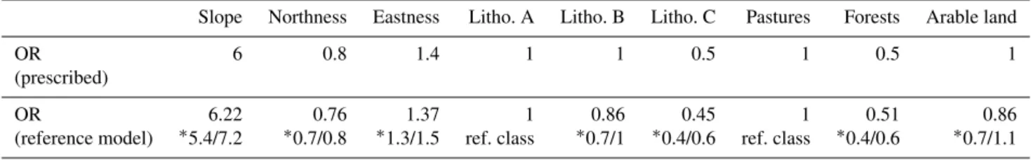
Table 1.Prescribed relationship between the predictors and the response variable for the synthetic data set expressed as odds ratios (OR) (first row). The model estimate (bottom row) was based on the synthetically generated landslide sample (see Fig. 3f) and a logistic regression model trained with the predictors slope, northness, eastness, lithology, land cover. OR for the predictor slope relate to a slope angle increase of 10◦, OR for both components of slope aspect (northness, eastness) to an orientation change of 45◦.
Slope Northness Eastness Litho. A Litho. B Litho. C Pastures Forests Arable land
OR 6 0.8 1.4 1 1 0.5 1 0.5 1
(prescribed)
OR 6.22 0.76 1.37 1 0.86 0.45 1 0.51 0.86
(reference model) ∗5.4/7.2 ∗0.7/0.8 ∗1.3/1.5 ref. class ∗0.7/1 ∗0.4/0.6 ref. class ∗0.4/0.6 ∗0.7/1.1
∗95 % confidence interval
each raster cell of the area to obtain a probability raster ex-pressing the predefined associations (Fig. 3f). A sampling ap-proach developed by Theobald et al. (2007) was adopted to spatially distribute landslide initiation zones (i.e. represented by points) according to the predefined relationships. More precisely, the mentioned probability raster was used to con-trol sampling intensity during the generation of 2000 spa-tially balanced landslide initiation points (i.e. raster cells with high probabilities are more likely selected as landslide loca-tion) (Theobald et al., 2007). This comparably high number of landslide points was chosen to assure a high explanatory power of the empirical results while simultaneously assuring computational feasibility. The resulting sample (Fig. 3f) was considered to represent an unbiased and accurate landslide inventory and used as presence data within all previously mentioned analyses (see Sects. 4.1 to 4.5). The similarity of prescribed relationships (OR in the first row of Table 1) and model estimates (OR in the second row of Table 1) indicated that the previously established associations were successfully describable by the logistic regression model fitted with arti-ficially generated data sets (i.e. response variable and predic-tors). Thus, we further considered this model as a useful ref-erence that reflects the “true” relation between the response and the respective environmental conditions.
5 Results
A first inspection of real and synthetic data sets revealed that landslides were more frequent on flatter slopes and less fre-quent on steeper slopes with a decreasing positional accuracy of the respective inventory (Figs. 2b, 3g). On average, slope angles of the original landslide locations were 4.1◦(real data)
and 4.6◦ (synthetic data) higher compared to the most
in-accurate inventory (mean error: 120 m). Landslide densities within lithological units changed comparably little when in-troducing the highest positional error (mean 120 m) into the inventories. Landslide densities within the Flysch decreased from 7.2 to 7 landslides per km2 while landslide densities observed for the Molasse remained unchanged (1 landslide per km2). An increasing landslide density was detected for
the Quaternary unit by introducing a mean positional error of 120 m (from 0.4 to 0.7 landslides per km2). The following changes in landslide densities were observed for the litho-logical units of the synthetically generated data set by intro-ducing a high positional error (mean: 120 m): The number of landslides per km2for unit A (respectively B) decreased from 33.3 (B: 14.1) to 31.4 (B: 12.7), while landslide density within the unit C increased from 13.3 to 14.9.
5.1 Modelled relationships
Modelled relationships obtained for the predictors slope an-gle, northness and eastness (for both data sets) and land cover (only synthetic data) indicated that the strength of association with landslide occurrence generally decreased with an increasing positional error of the inventory since the respective OR tended to approach the neutral value of 1 (Fig. 4a, c, d, f, g). Only the predictor lithology (Fig. 4b, e) did not show this trend.
Modelled associations remained nearly unchanged when simulating the smallest positional error (mean: 5 m) (Fig. 4). OR changes became noticeable for a simulated mean posi-tional error of 10 m (real data) respectively 50 m (synthetic data; compare OR with the dashed line in Fig. 4). Espe-cially, OR of the predictors slope (Fig. 4a, d) and lithol-ogy (Fig. 4b, e) provided quantitative evidence that the mod-els generated with real data exhibit a higher sensitivity to medium positional errors of the inventory (e.g. mean: 10, 20 m) compared to the apparently more robust synthetic models.
OR further exposed that a decreasing accuracy of landslide inventories was related to decreasing sensitivity of modelling results on slope angle (Fig. 4a, d). For instance, the suscepti-bility model generated with real data and with the unmodified inventory showed that the chances of a 10◦steeper slope to be
affected by future landsliding are 7.3 times higher compared to its 10◦flatter counterparts. The respective model generated
rela-S. Steger et al.: The propagation of inventory-based positional errors 2737
Figure 4.Estimated odds ratios (OR) for the models generated with differently accurate landslide inventories. ORs obtained for the predictors
slope(a, d), northness(c, f), eastness(c, f)and land cover(g)suggested a decreasing estimated effect of topographic and land cover variations
on modelling results with an increasing positional error of the inventory (i.e. ORs are approaching the no-effect threshold value 1). ORs of the lithology classes revealed decreasing modelled chances that the Molasse(b)respectively the unit B(e)may be affected by future landsliding.
tion (OR > 1) between landslide occurrence and the inclina-tion of a slope. OR obtained for the lithology layers revealed major changes for the Molasse (real data) respectively the lithological unit B (synthetic data) (Fig. 4b, e). The chances that those units will be affected by future landslides were modelled to be considerably lower (i.e. most distant from the threshold of 1) whenever the respective model was generated with the most inaccurate data sets.
5.2 Visual appearance of maps
A visual inspection of landslide susceptibility maps generally confirmed that the respective modelled relationships were vi-sually recognizable in the predicted susceptibility patterns. Thus, a high positional error of the inventory (mean error: 120 m) was observed to result in susceptibility maps that were less influenced by local slope angle and slope aspect variations. Ultimately, this led to more uniformly appear-ing susceptibility patterns at slope scale (e.g. Fig. 5f). Flat-ter slopes were generally predicted as more susceptible and steepest slopes as less susceptible with an increasing posi-tional inventory-based error (Fig. 5). The declining effect of local slope variations was accompanied by an increasing vis-ibility of lithological transitions. Especially the model gener-ated with real data and the most inaccurate inventory (Fig. 5f) depicted this tendency by strongly accentuating the silhou-ettes of the Flysch Zone (see Fig. 1c).
5.3 Predictive performance
Predictive performances decreased with a decreasing posi-tional accuracy of the inventories (CV and SCV in Fig. 5). However, models generated with a mean inventory-based er-ror of 50 m still produced AUROCs of 0.76 (CV; real data) re-spectively 0.83 (synthetic data). Non-spatially assessed me-dian AUROCs were observed to decrease from 0.85 (real data) and 0.86 (synthetic data) to 0.69 (real data) and 0.75 (synthetic data) (CV in Fig. 5). The general trend of de-creasing prediction skills with an inde-creasing positional error was exposed by both partitioning techniques, namely CV and SCV. In analogy to observations of the modelled relation-ships, we observed a first distinct performance drop (AU-ROC decrease of > 0.1) for the models generated with an inventory-based positional mean error of 10 m (real data) re-spectively 50 m (synthetic data).
Figure 5.Landslide susceptibility maps (for the location of the cutouts refer to the red boxes) of models generated with differently accurate
inventories (rows) for the real data (left column) and the synthetic data (right column). Corresponding predictive performances (median AUROC for CV and SCV) and the quantitative comparison with the original landslide positions (0 in Fig. 5) are given in the respective white boxes. The cutouts additionally show the location of the positionally erroneous inventories (white dots) used as input for the respective models and the position of the original inventory (red dot). Note that maps generated with the most inaccurate inventory(f, l)are characterized by a locally more uniform spatial pattern.
5.4 Predictor importance
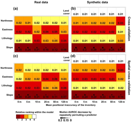
The findings provided quantitative indications that the re-sults of variable importance assessments obtained by multi-ple variable statistical landslide susceptibility models are not only related to underlying geomorphic processes, but also to positional errors inherent in the underlying landslide inven-tories. The general ranking of predictors within the models generated with real data changed first for a mean positional accuracy of 10 m (CV) respectively 5 m (SCV) (Fig. 6a, c). In contrast, the ranking of predictors remained unchanged for the models generated with synthetic data sets up to a mean positional error of 120 m (Fig. 6b, d).
Slope had the greatest variable importance in all situa-tions, revealing that this environmental factor played the cen-tral role to predict landslide susceptibility within each model. However, an interpretation of AUROC decreases (Fig. 6) also suggested that the dominance of this predictor diminished as positional error increased (e.g. from 0.25 to 0.08 in Fig. 6a). An opposite, but less pronounced tendency was observed for the predictor lithology (e.g. from 0.01 to 0.05 in Fig. 6a). The
importance of the predictors slope (CV: 0.08; SCV: 0.07) and lithology (CV: 0.05; SCV: 0.06) was similar whenever the models were generated with the most inaccurate inventory and with real data.
6 Discussion
S. Steger et al.: The propagation of inventory-based positional errors 2739
Figure 6.Permutation-based variable importance for the respective reference models (0 m) and models generated with positionally erroneous
inventories (5–120 m) for the real data sets(a, c)and the synthetic data(b, d)obtained by CV(a, b)and SCV(c, d). The relative ranking indicates that slope was the most influential predictor for each model while its estimated importance constantly decreased with an increasing inventory-based positional error (see Median AUROC decrease). The estimated importance of lithology slightly increases with a growing inventory-based positional inaccuracy.
However, the systematic comparisons also suggested that interdependencies between inventory-based errors and sub-sequent modelling and validation results are complex. Thus, an identification of a generally valid threshold (i.e. the posi-tional error should not exceed x metres), which separates ac-ceptable models from unacac-ceptable ones, was considered to be inappropriate. The findings provided valuable indications that the propagation of inventory-based errors is not only de-termined by the degree of positional inaccuracy inherent in a landslide data set, but also by a combination of additional factors. Those aspects include (i) the spatial representation of landslides and the environment (see Sect. 6.2), (ii) landslide sizes (see Sect. 6.2), (iii) the characteristics of the study area (see Sect. 6.3), (iv) the selection of a classification method (see Sect. 6.4) and (v) an interplay of predictors within mul-tiple variable models (see Sect. 6.5).
6.1 Usefulness of an additional modelling with synthetic data
the effect of inventory-based errors on modelling results and cross-check our findings. Furthermore, observed differences between modelling results obtained from the real data sets and the synthetically generated data (e.g. differences in OR-drops; see Fig. 4) were helpful to move our attention to re-lated important model-influencing aspects (e.g. characteris-tics of the study area; see Sect. 6.3).
6.2 The spatial representation of input data and landslide size
The available landslide point inventory represents the scarp locations of mainly smaller landslide features, which tend to exhibit a distinct steep and concave morphology in compari-son to its surroundings (Petschko et al., 2016). Consequently, already small changes in the point position (e.g. 5 m) may lead to the tendency that the respective features are, in the case of high-resolution slope data (e.g. 1 m×1 m), displaced into their usually flatter vicinities. However, those immediate neighbourhoods may be represented by identical lithologies, land cover classes or soil types due to a typically coarser spa-tial resolution of the underlying data sets (Cascini, 2008; Van Westen et al., 2008).
We argue that the applied modelling resolution of input data might not only affect the relative importance of pre-dictors within a landslide susceptibility model (Catani et al., 2013), but also how spatial inventory-based errors are prop-agated into the final modelling results. For instance, the re-sampling of the present DTM from 1 m×1 m to the mod-elling resolution of 10 m×10 m was related to an enlarge-ment of the area covered by one grid cell (i.e. 1 to 100 m2) and a generalization of the topography. This combination in-creased the chances that nearby observations (e.g. 5 m dis-tance from original location) were represented by an identi-cal grid cell or cells with similar values (e.g. of slope) to the respective original location. Therefore, slope angles of land-slide locations (real data) derived from a 10 m-raster were on average just 0.2◦lower for a mean inventory-based
inac-curacy of 5 m compared to the unmodified inventory. These similarities were expected to mainly cause the observed ef-fect that an average inventory-based error of 5 m did almost not affect modelled relationships (Fig. 4). Thus, we argue that a resampling of predictors to a coarser resolution might not only help to reduce the impact of local topographic varia-tions related to post-failure condivaria-tions (condivaria-tions after land-slide occurrence) or data noisiness (Petschko et al., 2014a; Van Den Eeckhaut et al., 2006; Van Westen et al., 2008), but also to reduce the impact of smaller inventory-based posi-tional errors on the results of a grid-based statistical landslide susceptibility model.
A very high mean positional error of an inventory (e.g. 120 m) may require a correspondingly higher generalization of the topographic variables, such as slope angle or slope as-pect, to enhance the chances that the respective landslide ob-servation is still represented by an identical respectively
simi-lar grid cell. However, those high simplifications may as well lead to the effect that actual important landslide-influencing morphological features disappear within the derivatives of a strongly resampled terrain model.
The chances that an inaccurately mapped landslide-point may still be located within the boundaries of a corresponding landslide may as well increase with an increasing size of the respective landslides. However, statistically predicting land-slide susceptibility for mainly larger events may nonethe-less require a substantial generalization of a grid-based to-pography, because the respective pre-failure conditions may considerably differ from the conditions after landslide oc-currence (Hussin et al., 2016; Süzen Lüfti and Doyuran, 2004; Van Den Eeckhaut et al., 2006). Again, corresponding simplifications (i.e. resampling) might result in topographi-cal predictors of little practitopographi-cal use. Such discrepancies (i.e. between pre-failure and post-failure topographies) may be counteracted for accurately mapped inventories by approxi-mating the terrain before landslide occurrence (e.g. Van Den Eeckhaut et al., 2006). However, such approaches are likely to be inapplicable whenever only positionally erroneous in-ventories are available.
We finally recommend that an expected small to moderate positional inaccuracy inherent in a landslide inventory (e.g. 5 to 20 m) might partly be counteracted by resampling the respective grid-based data sets to a spatial resolution higher than the expected mean positional inaccuracy. An alterna-tive spatial representation of the environment (e.g. terrain units, first-order catchments) (Alvioli et al., 2016; Bell et al., 2014b; Guzzetti et al., 1999) might be most expedient when-ever modelling with highly inaccurate landslide inventories or erroneous inventories that mainly consist of large events is envisaged. The associated high generalization of environ-mental conditions within terrain-unit based models might be one reason for earlier observations that susceptibility maps generated from inventories with considerable positional dis-agreements appeared and performed similarly (Ardizzone et al., 2002). In this respect, recent developments which allow an automatic, but controllable (e.g. sizes of units) subdivi-sions of the terrain into slope units (Alvioli et al., 2016) might prove highly useful. It is, however, important to en-sure that the respective landslides are still located within the unit where they were initiated (Bell et al., 2014b). Which ap-proach to apply also depends on the ultimate aim of the final susceptibility maps, e.g. either to be used in spatial planning strategies or as part of regional landslide early warning sys-tems.
6.3 The characteristics of the study area
S. Steger et al.: The propagation of inventory-based positional errors 2741 locations (e.g. slope angles in Fig. 2b). In the more strongly
generalized synthetic area, in contrast, such changes in mod-elled relationships were hardly noticeable up to a mean po-sitional error of 50 m (3-D view in Figs. 3a, 4d). The dif-ferences between the synthetic data and the real data were interpreted as evidence that the geomorphic characteristics of a study area plays as well a major role on how inventory-based inaccuracies may be propagated into modelling results. We inferred that as long as the resolution of the data is gen-eralized to mainly present pre-failure conditions, grid-based models generated for undulating and smooth landscapes (e.g. Flysch Zone of Lower Austria) might tend to be less af-fected by smaller positional errors of the inventory com-pared to sites featuring sharp topographic transitions (e.g. ter-raced landscapes, cuesta landscapes, limestone areas). Based on the results we inferred that the influence of an identical inventory-based mean positional error (e.g. 20 m) on subse-quent modelling results may be considerably higher for ar-eas exhibiting a topographically more complex terrain. This complexity is on one hand dependent on how a study site is represented (see Sect. 6.2), but also on the characteristics of the study area itself.
6.4 An additional argument on why model overfitting should be avoided
An aspect worth further consideration is whether different classification techniques are to a different extent affected by positional inaccuracies of landslide inventories. In particu-lar, non-linear statistical models (e.g. Generalized additive models, multivariate adaptive regression splines) or flexible machine learning techniques (e.g. Support Vector Machines, Decision Trees, Random Forest) are increasingly used be-cause of possible gains in predictive performance (Ballabio and Sterlacchini, 2012; Catani et al., 2013; Felicísimo et al., 2013; Tien Bui et al., 2012), but they bear a higher risk of overfitting to training data (Brenning, 2005, 2012a; Goetz et al., 2015a; Steger et al., 2016). In analogy to a generalized representation of the study area (see Sect. 6.2), we expect that a higher degree of model generalization, as provided by the less flexible techniques, may provide a certain level of protection against learning, i.e. overfitting to, errors originat-ing from a landslide inventory.
Thus, this study supports the statement that an application of strongly generalizing classifiers might still be valuable in the context of landslide susceptibility modelling (Brenning, 2012a; Goetz et al., 2015a; Steger et al., 2016) while we sus-pect that strongly overfitting classifiers are likely to repro-duce inventory-based errors. This assumption is supported by earlier research, which showed that logistic regression-based landslide susceptibility models generated with rather different landslide inventories produced similar predictive performances and landslide susceptibility maps (Zêzere et al., 2009). Furthermore, Ardizzone et al. (2002) concluded
that statistical models may as well substantially minimize the effect of data errors on landslide susceptibility models. 6.5 Considerations of an interplay of predictors within
multiple variable models
Logistic regression models, like other multiple variable clas-sifiers, try to maximize the probability of obtaining the ob-servations (landslide presence or landslide absence) accord-ing to the data provided (Hosmer and Lemeshow, 2000). The present findings (i.e. OR and predictor importance) provided quantitative indications that the applied models counteracted the diminishing explanatory power of topographic variations (especially slope angle) by adjusting the weights assigned to the coarser scaled predictor lithology.
For instance, the logistic regression models produced with real data and with the unmodified inventory did not strongly accentuate differences in landslide susceptibility (see OR in Fig. 4b) between the Flysch (7.2 landslides per km2 ) and the Molasse (1 landslide per km2) since the respec-tive models accounted for the fact that the Flysch Zone is considerably steeper (mean slope 12.3◦) compared to the
Molasse (5.1◦). Even though landslide densities observed
for those units remained nearly unchanged when simulat-ing an inventory-based-error (i.e. Flysch 7 and Molasse 1 landslide per km2for the 120 m mean error), modelled rela-tionships increasingly emphasized differences between those units (Fig. 4b). Thus, we inferred that the respective mod-els were decreasingly capable to account for local topo-graphic variations (OR of slope are approaching the thresh-old of 1) with an increasing positional error of the inven-tory and subsequently were increasingly dependent on dif-ferences describable by other predictors (e.g. landslide den-sities for lithological units). Those tendencies were also dis-cernible for the synthetic data set, ultimately due to deterio-rating topographical effects (see Fig. 4) and dissimilar land-slide densities between lithological units (see Sect. 5). Vari-able importance assessments (e.g. decreasing importance of slope and increasing importance of lithology in Fig. 6) and the appearance of the final maps (e.g. striking appearance of the Flysch in Fig. 5f) further exposed these distortions. This study underlines that besides the applied raster reso-lution (Catani et al., 2013), also the inventory-based posi-tional accuracy influences how strongly a predictor appears to discriminate landslide-presences from landslide-absences. Consequently, we argue that potential inventory-based posi-tional errors should addiposi-tionally be taken into account, when a process-based geomorphic interpretation of statistical land-slide susceptibility models is envisaged (Brenning et al., 2015; Vorpahl et al., 2012).
6.6 Misleading performance estimates
approaches a distribution of complete spatial randomness (Cressie, 2015). Thus, statistically discriminating landslide locations from non-landslide locations becomes increasingly difficult since non-landslide observations are regularly rep-resented by random spatial observations (e.g. Conoscenti et al., 2016; Goetz et al., 2015a). The observed decreasing predictive performances provided quantitative evidence for this assumption (CV and SCV in Fig. 5). The tendency to-wards diminishing differences between landslide presences and absences were also reflected by conditional frequencies of slope angles (Figs. 2b, 3g) and OR of topographic param-eters (Fig. 4).
The spatial pattern of landslide susceptibility maps (e.g. cutouts in Fig. 5) visually highlighted that all models estab-lished a positive relationship between landslide occurrence and slope angle (ORs > 1.9 in Fig. 4a, d) while the litho-logical units Flysch (real data) respectively the unit A (syn-thetic data) were consistently predicted as most suscepti-ble (Fig. 4b, e). Thus, all models predicted that the steep-est parts of the Flysch Zone (respectively unit A) are highly prone to landsliding, even though the underlying landslide-presences (white dots in Fig. 5) were increasingly located on considerably flatter slopes (e.g. Figs. 2b, 3g). In analogy, the flattest parts covered by Quaternary sediments (respec-tively unit C) were consistently predicted as the most stable locations. From this perspective, it might become clear that models generated with erroneous inventories performed well (all AUROCs > 0.84) in predicting the original landslide po-sition (see 0 in Fig. 5). This observation is consistent with our suggestion that strongly generalizing classifiers might also reduce the effect of inventory-based errors on modelling re-sults (see Sect. 6.4; Ardizzone et al., 2002). However, val-idation results that were based on a landslide subsample of the data set used to generate the model (as within most stud-ies) revealed apparently lower predictive performances (CV, SCV in Fig. 5). Thus, this study provides another example that misleading performance estimates may follow whenever a landslide susceptibility model is generated and validated with erroneous landslide inventories (Steger et al., 2016).
This study further underlined that the predictive perfor-mance of a statistical landslide susceptibility model is just one of many indicators of the quality and reliability of a spa-tial prediction model (Fressard et al., 2014; Guzzetti et al., 2006; Lobo et al., 2008; Petschko et al., 2014a; Rossi et al., 2010; Steger et al., 2016). Thus, we consider a differentiated evaluation of input data qualities and modelling results (i.e. quantitative and expert-based) as an necessary supplement to get insights into limitations and the reliability of subsequent modelling results (Demoulin and Chung, 2007; Fressard et al., 2014; Guzzetti et al., 2006; Petschko et al., 2014a; Steger et al., 2016).
7 Conclusion and final recommendations
There is no doubt that the explanatory power of a landslide susceptibility analysis increases with an increasing quality of the underlying landslide inventory (Fressard et al., 2014; Galli et al., 2008; Guzzetti et al., 2006; Petschko et al., 2016; Steger et al., 2016; Van Westen et al., 2008). The present find-ings highlighted that positionally erroneous landslide inven-tories affected modelled relationships, variable importance assessments and the explanatory power of conventional pre-dictive performance estimates of a statistical landslide sus-ceptibility model. We found valuable evidence that the im-pact of inventory-based positional errors on modelling re-sults is not only dependent on the degree of inaccuracy in-herent in the respective landslide-presence data but also on an interplay of other model-influencing aspects. Aside from the size (i.e. small vs. large landslides) and spatial represen-tation of landslides (i.e. landslide scarp vs. landslide body), the spatial representation of the environment (i.e. raster res-olution, terrain unit) was also expected to determine how a specific positional error was propagated into the final re-sults. Furthermore, also the morphological characteristics of the study area (i.e. undulating landscape vs. landscape with sharp transitions) and the applied classification method (i.e. strongly generalizing vs. highly flexible classifiers) are be-lieved to control the extent of potentially misleading mod-elling results.
The present findings indicate that the propagation of inventory-based positional inaccuracies into modelling re-sults can be reduced by selecting an appropriate study de-sign. Thus, we advise to accept inventory-based errors as un-avoidable and then seek to obtain in-depth information on the potential limitations of present data sets. A subsequent im-provement of the respective data set (e.g. updated mapping) should be the first step. For the likely case that modelling with positionally imperfect inventories cannot be avoided (e.g. Bell et al., 2014b; Van Den Eeckhaut et al., 2011), we recommend to generalize input data to a coarser scale (e.g. resampling of predictors or using an alternative representa-tion of the environment; see Sect. 6.2) while opting for mod-elling techniques that simplify observed associations (e.g. lo-gistic regression; see Sect. 6.4). The potential presence of inventory-based errors should always be taken into account since subsequent performance estimates (see Sect. 6.6), mod-elled relationships and variable importance (see Sect. 6.5) are likely to be distorted whenever the underlying models were generated with positionally erroneous landslide inventories.
S. Steger et al.: The propagation of inventory-based positional errors 2743
the paper.
Edited by: P. Tarolli
Reviewed by: two anonymous referees
References
Alvioli, M., Marchesini, I., Reichenbach, P., Rossi, M., Ardiz-zone, F., Fiorucci, F., and Guzzetti, F.: Automatic delineation of geomorphological slope units withr.slopeunits v1.0
and their optimization for landslide susceptibility modeling, Geosci. Model Dev., 9, 3975–3991, doi:10.5194/gmd-9-3975-2016, 2016.
Ardizzone, F., Cardinali, M., Carrara, A., Guzzetti, F., and Re-ichenbach, P.: Impact of mapping errors on the reliability of landslide hazard maps, Nat. Hazards Earth Syst. Sci., 2, 3–14, doi:10.5194/nhess-2-3-2002, 2002.
Atkinson, P. M. and Massari, R.: Generalised linear modelling of susceptibility to landsliding in the central Apennines, Italy, Com-put. Geosci., 24, 373–385, 1998.
Atkinson, P., Jiskoot, H., Massari, R., and Murray, T.: Generalized linear modelling in geomorphology, Earth Surf. Proc. Land., 23, 1185–1195, 1998.
Ballabio, C. and Sterlacchini, S.: Support Vector Machines for Landslide Susceptibility Mapping: The Staffora River Basin Case Study, Italy, Math. Geosci., 44, 47–70, doi:10.1007/s11004-011-9379-9, 2012.
Beguería, S.: Validation and Evaluation of Predictive Models in Hazard Assessment and Risk Management, Nat. Hazards, 37, 315–329, doi:10.1007/s11069-005-5182-6, 2006.
Bell, R., Petschko, H., Röhrs, M., and Dix, A.: Assessment of landslide age, landslide persistence and human impact using airborne laser scanning digital terrain models, Geografiska An-naler: Series A, Phys. Geogr., 94, 135–156, doi:10.1111/j.1468-0459.2012.00454.x, 2012.
Bell, R., Petschko, H., Proske, H., Leopold, P., Heiss, G., Bauer, C., Goetz, J., Granica, K., and Glade T.: Methodenentwick-lung zur Gefährdungsmodellierung von Massenbewegungen in Niederösterreich – MoNOE, Final project report, 224 pp., Vi-enna, 2014a.
Bell, R., Cepeda, J., and Devoli, G.: Landslide susceptibility mod-eling at catchment level for improvement of the landslide early warning system in Norway, in: Conference Proceedings of the World Landslide Forum 3, vol. 4: Discussion Session, Beijing, China, 2014b.
Blahut, J., Van Westen, C. J., and Sterlacchini, S.: Analy-sis of landslide inventories for accurate prediction of debris-flow source areas, Geomorphology, 119, 36–51, doi:10.1016/j.geomorph.2010.02.017, 2010.
Brabb, E. E.: Innovative approaches to landslide hazard mapping. 4th International Symposium on Landslides, 16–21 September, 307–324, Toronto, 1984.
Brenning, A.: Spatial prediction models for landslide hazards: re-view, comparison and evaluation, Nat. Hazards Earth Syst. Sci., 5, 853–862, doi:10.5194/nhess-5-853-2005, 2005.
Brenning, A.: Benchmarking classifiers to optimally integrate ter-rain analysis and multispectral remote sensing in automatic
rock glacier detection, Remote Sens. Environ., 113, 239–247, doi:10.1016/j.rse.2008.09.005, 2009.
Brenning, A.: Improved spatial analysis and prediction of land-slide susceptibility: Practical recommendations, in: Landland-slides and Engineered Slopes: Protecting Society through Improved Understanding, edited by: Eberhardt, E., Froese, C., Turner, A. K., and Leroueil, S., Tylor and Francis, Banff, Alberta, Canada, 789–795, 2012a.
Brenning, A.: Spatial cross-validation and bootstrap for the assessment of prediction rules in remote sensing: The R package sperrorest, in: Geoscience and Remote Sens-ing Symposium (IGARSS), 2012 IEEE International, 5372– 5375, available at: http://ieeexplore.ieee.org/xpls/abs_all.jsp? arnumber=6352393 (last access: 22 April 2016), 2012b. Brenning, A., Schwinn, M., Ruiz-Páez, A. P., and Muenchow, J.:
Landslide susceptibility near highways is increased by 1 order of magnitude in the Andes of southern Ecuador, Loja province, Nat. Hazards Earth Syst. Sci., 15, 45–57, doi:10.5194/nhess-15-45-2015, 2015.
Cascini, L.: Applicability of landslide susceptibility and haz-ard zoning at different scales, Eng. Geol., 102, 164–177, doi:10.1016/j.enggeo.2008.03.016, 2008.
Catani, F., Lagomarsino, D., Segoni, S., and Tofani, V.: Landslide susceptibility estimation by random forests technique: sensitivity and scaling issues, Nat. Hazards Earth Syst. Sci., 13, 2815–2831, doi:10.5194/nhess-13-2815-2013, 2013.
Chung, C.-J. F. and Fabbri, A. G.: Validation of spatial prediction models for landslide hazard mapping, Nat. Hazards, 30, 451– 472, 2003.
Conoscenti, C., Rotigliano, E., Cama, M., Caraballo-Arias, N. A., Lombardo, L. and Agnesi, V.: Exploring the effect of absence se-lection on landslide susceptibility models: A case study in Sicily, Italy, Geomorphology, 261, 222–235, 2016.
Corominas, J., Van Westen, C., Frattini, P., Cascini, L., Malet, J.-P., Fotopoulou, S., Catani, F., Van Den Eeckhaut, M., Mavrouli, O., Agliardi, F., Pitilakis, K., Winter, M. G., Pastor, M., Ferlisi, S., Tofani, V., Hervás, J., and Smith, J. T.: Recommendations for the quantitative analysis of landslide risk, B. Eng. Geol. Environ., 73, 209–263, doi:10.1007/s10064-013-0538-8, 2013.
Cressie, N.: Statistics for spatial data, John Wiley & Sons, 2015. Demoulin, A. and Chung, C.-J. F.: Mapping landslide
sus-ceptibility from small datasets: A case study in the Pays de Herve (E Belgium), Geomorphology, 89, 391–404, doi:10.1016/j.geomorph.2007.01.008, 2007.
Eder, A., Sotier, B., Klebinder, K., Sturmlechner, R., Dorner, J., Markart, G., Schmid, G., and Strauss, P.: Hydrologische Bo-denkenndaten der Böden Niederösterreichs – Endbericht, Hydro-BodNÖ. BAW, BFW, 2011.
Ermini, L., Catani, F., and Casagli, N.: Artificial Neural Networks applied to landslide susceptibility assessment, Geomorphology, 66, 327–343, doi:10.1016/j.geomorph.2004.09.025, 2005. Fabbri, A. G., Chung, C.-J. F., Cendrero, A., and Remondo, J.: Is
prediction of future landslides possible with a GIS?, Nat. Haz-ards, 30, 487–503, 2003.
Fell, R., Corominas, J., Bonnard, C., Cascini, L., Leroi, E., and Savage, W. Z.: Guidelines for landslide susceptibility, hazard and risk zoning for land use planning, Eng. Geol., 102, 85–98, doi:10.1016/j.enggeo.2008.03.022, 2008.
Frattini, P., Crosta, G., and Carrara, A.: Techniques for evaluating the performance of landslide susceptibility models, Eng. Geol., 111, 62–72, doi:10.1016/j.enggeo.2009.12.004, 2010.
Fressard, M., Thiery, Y., and Maquaire, O.: Which data for quanti-tative landslide susceptibility mapping at operational scale? Case study of the Pays d’Auge plateau hillslopes (Normandy, France), Nat. Hazards Earth Syst. Sci., 14, 569–588, doi:10.5194/nhess-14-569-2014, 2014.
Galli, M., Ardizzone, F., Cardinali, M., Guzzetti, F., and Reichen-bach, P.: Comparing landslide inventory maps, Geomorphology, 94, 268–289, doi:10.1016/j.geomorph.2006.09.023, 2008. Glade, T., Anderson, M., and Crozier, M. J. (Eds.): Landslide hazard
and risk, J. Wiley, Chichester, West Sussex, England?, Hoboken, NJ, 2005.
Goetz, J. N., Brenning, A., Petschko, H., and Leopold, P.: Evalu-ating machine learning and statistical prediction techniques for landslide susceptibility modeling, Comput. Geosci., 81, 1–11, doi:10.1016/j.cageo.2015.04.007, 2015a.
Goetz, J. N., Guthrie, R. H., and Brenning, A.: Forest harvesting is associated with increased landslide activity during an extreme rainstorm on Vancouver Island, Canada, Nat. Hazards Earth Syst. Sci., 15, 1311–1330, doi:10.5194/nhess-15-1311-2015, 2015b. Gorsevski, P. V., Gessler, P. E., Foltz, R. B., and Elliot, W. J.: Spatial
prediction of landslide hazard using logistic regression and ROC analysis, Transactions in GIS, 10, 395–415, 2006.
Guzzetti, F., Carrara, A., Cardinali, M., and Reichenbach, P.: Land-slide hazard evaluation: a review of current techniques and their application in a multi-scale study, Central Italy, Geomorphology, 31, 181–216, 1999.
Guzzetti, F., Reichenbach, P., Cardinali, M., Galli, M., and Ardizzone, F.: Probabilistic landslide hazard assess-ment at the basin scale, Geomorphology, 72, 272–299, doi:10.1016/j.geomorph.2005.06.002, 2005.
Guzzetti, F., Reichenbach, P., Ardizzone, F., Cardinali, M. and Galli, M.: Estimating the quality of landslide
susceptibility models, Geomorphology, 81, 166–184,
doi:10.1016/j.geomorph.2006.04.007, 2006.
Guzzetti, F., Mondini, A. C., Cardinali, M., Fiorucci, F., San-tangelo, M. and Chang, K.-T.: Landslide inventory maps: New tools for an old problem, Earth-Sci. Rev., 112, 42–66, doi:10.1016/j.earscirev.2012.02.001, 2012.
Harp, E. L., Keefer, D. K., Sato, H. P., and Yagi, H.: Landslide in-ventories: the essential part of seismic landslide hazard analyses, Eng. Geol., 122, 9–21, 2011.
Heckmann, T., Gegg, K., Gegg, A., and Becht, M.: Sample size mat-ters: investigating the effect of sample size on a logistic regres-sion susceptibility model for debris flows, Nat. Hazards Earth Syst. Sci., 14, 259–278, doi:10.5194/nhess-14-259-2014, 2014. Hosmer, D. W. and Lemeshow, S.: Applied Logistic Regression,
John Wiley & Sons, New York, 2000.
Hussin, H. Y., Zumpano, V., Reichenbach, P., Sterlacchini, S., Micu, M., Van Westen, C., and B˘alteanu, D.: Different landslide sampling strategies in a grid-based bi-variate sta-tistical susceptibility model, Geomorphology, 253, 508–523, doi:10.1016/j.geomorph.2015.10.030, 2016.
Hutton, J.: X. Theory of the Earth; or an Investigation of the Laws observable in the Composition, Dissolution, and Restoration of Land upon the Globe, Earth Env. Sci. T. R. So., 1, 209–304, doi:10.1017/S0080456800029227, 1788.
King, G. and Zeng, L.: Logistic regression in rare events data, Polit. Anal., 9, 137–163, 2001.
Lobo, J. M., Jiménez-Valverde, A., and Real, R.: AUC: a mislead-ing measure of the performance of predictive distribution mod-els, Global Ecol. Biogeogr., 17, 145–151, doi:10.1111/j.1466-8238.2007.00358.x, 2008.
Malamud, B. D., Turcotte, D. L., Guzzetti, F., and Reichenbach, P.: Landslide inventories and their statistical properties, Earth Surf. Proc. Land., 29, 687–711, doi:10.1002/esp.1064, 2004. Petschko, H., Brenning, A., Bell, R., Goetz, J., and Glade, T.:
Assessing the quality of landslide susceptibility maps – case study Lower Austria, Nat. Hazards Earth Syst. Sci., 14, 95–118, doi:10.5194/nhess-14-95-2014, 2014a.
Petschko, H., Bell, R., and Glade, T.: Relative Age Estimation at Landslide Mapping on LiDAR Derivatives: Revealing the Ap-plicability of Land Cover Data in Statistical Susceptibility Mod-elling, in: Landslide Science for a Safer Geoenvironment, edited by: Sassa, K., Canuti, P., and Yin, Y., 337–343, Springer Interna-tional Publishing, doi:10.1007/978-3-319-05050-8_53 (last ac-cess: 26 July 2016), 2014b.
Petschko, H., Bell, R., and Glade, T.: Effectiveness of visually ana-lyzing LiDAR DTM derivatives for earth and debris slide inven-tory mapping for statistical susceptibility modeling, Landslides, 13, 857–872, doi:10.1007/s10346-015-0622-1, 2016.
R Core Team: R: A language and environment for statistical com-puting, R Foundation for Statistical Comcom-puting, Vienna, avail-able at: http://www.R-project.org/ (last access: August 2016), 2014.
Remondo, J., González, A., De Terán, J. R. D., Cendrero, A., Fab-bri, A., and Chung, C.-J. F.: Validation of landslide susceptibility maps; examples and applications from a case study in Northern Spain, Nat. Hazards, 30, 437–449, 2003.
Rickli, C., Zürcher, K., Frey, W., and Lüscher, P.: Wirkungen des Waldes auf oberflächennahe Rutschprozesse, Schweizerische Zeitschrift für Forstwesen, 153, 437–445, 2002.
Rossi, M., Guzzetti, F., Reichenbach, P., Mondini, A. C., and Peruccacci, S.: Optimal landslide susceptibility zonation based on multiple forecasts, Geomorphology, 114, 129–142, doi:10.1016/j.geomorph.2009.06.020, 2010.
Ruß, G. and Brenning, A.: Spatial Variable Importance Assessment for Yield Prediction in Precision Agriculture, in: Advances in Intelligent Data Analysis IX, edited by: Cohen, P. R., Adams, N. M., and Berthold, M. R., 184–195, Springer Berlin Heidel-berg, doi:10.1007/978-3-642-13062-5_18 (last access: 12 Au-gust 2016), 2010.
Santangelo, M., Marchesini, I., Bucci, F., Cardinali, M., Fiorucci, F., and Guzzetti, F.: An approach to reduce mapping errors in the production of landslide inventory maps, Nat. Hazards Earth Syst. Sci., 15, 2111–2126, doi:10.5194/nhess-15-2111-2015, 2015. Schweigl, J. and Hervás, J.: Landslide mapping in Austria, JRC
S. Steger et al.: The propagation of inventory-based positional errors 2745
Schwenk, H.: Massenbewegungen in Niederösterreich 1953–1990, Geologische Bundesanstalt, Wien, 1992.
Skoda, G. and Lorenz, P.: Mittlere Jahresniederschlagshöhe – Modellrechnung mit unkorrigierten Daten, Hydrologischer Atlas Österreich 2007, Erläuterungsblatt 2.2, 2007.
Steger, S., Bell, R., Petschko, H., and Glade, T.: Evaluating the Effect of Modelling Methods and Landslide Inventories Used for Statistical Susceptibility Modelling, in: Engineering Geol-ogy for Society and Territory – Volume 2, edited by: Lollino, G., Giordan, D., Crosta, G. B., Corominas, J., Azzam, R., Wa-sowski, J., and Sciarra, N., 201–204, Springer International Pub-lishing, available at: http://link.springer.com/chapter/10.1007/ 978-3-319-09057-3_27 (last access: 16 August 2016), 2015. Steger, S., Brenning, A., Bell, R., Petschko, H., and Glade,
T.: Exploring discrepancies between quantitative valida-tion results and the geomorphic plausibility of statistical landslide susceptibility maps, Geomorphology, 262, 8–23, doi:10.1016/j.geomorph.2016.03.015, 2016.
Strobl, C., Boulesteix, A.-L., Zeileis, A., and Hothorn, T.: Bias in random forest variable importance measures: Illus-trations, sources and a solution, BMC Bioinformatics, 8, 25, doi:10.1186/1471-2105-8-25, 2007.
Süzen Lüfti, M. L. and Doyuran, V.: A comparison of the GIS based landslide susceptibility assessment methods: multivariate versus bivariate, Environ. Geol., 45, 665–679, doi:10.1007/s00254-003-0917-8, 2004.
Theobald, D. M., Stevens, D. L., White, D., Urquhart, N. S., Olsen, A. R. and Norman, J. B.: Using GIS to Generate Spatially Bal-anced Random Survey Designs for Natural Resource Applica-tions, Environ. Manage., 40, 134–146, doi:10.1007/s00267-005-0199-x, 2007.
Tien Bui, D., Pradhan, B., Lofman, O., and Revhaug, I.: Landslide Susceptibility Assessment in Vietnam Using Support Vector Ma-chines, Decision Tree, and Naive Bayes Models, Math. Probl. Eng., 2012, e974638, doi:10.1155/2012/974638, 2012.
Van Den Eeckhaut, M., Vanwalleghem, T., Poesen, J., Govers, G., Verstraeten, G., and Vandekerckhove, L.: Prediction of landslide susceptibility using rare events logistic regression: A case-study in the Flemish Ardennes (Belgium), Geomorphology, 76, 392– 410, doi:10.1016/j.geomorph.2005.12.003, 2006.
Van Den Eeckhaut, M., Hervás, J., Jaedicke, C., Malet, J.-P., Mon-tanarella, L. and Nadim, F.: Statistical modelling of Europe-wide landslide susceptibility using limited landslide inventory data, Landslides, 9, 357–369, doi:10.1007/s10346-011-0299-z, 2011. Vorpahl, P., Elsenbeer, H., Märker, M., and Schröder, B.:
How can statistical models help to determine driv-ing factors of landslides?, Ecol. Model., 239, 27–39, doi:10.1016/j.ecolmodel.2011.12.007, 2012.
Wessely, G., Draxler, I., Gangl, G., Gottschling, P., Heinrich, M., Hofmann, T., Lenhardt, W., Matura, A., Pavuza, R., Peresson, H., and Sauer, R.: Geologie der österreichischen Bundesländer – Niederösterreich, Geologische Bundesanstalt, Wien, 2006. Van Westen, C. J., Castellanos, E., and Kuriakose, S. L.:
Spa-tial data for landslide susceptibility, hazard, and vulnera-bility assessment: An overview, Eng. Geol., 102, 112–131, doi:10.1016/j.enggeo.2008.03.010, 2008.
Wu, X., Chen, X., Zhan, F. B., and Hong, S.: Global research trends in landslides during 1991–2014: a bibliometric analysis, Land-slides, 12, 1215–1226, doi:10.1007/s10346-015-0624-z, 2015. Zêzere, J., Henriques, C. S., Garcia, R. A. C., and Piedade, A.: