Control of Limit Cycle Oscillation in a Three Degrees of Freedom Airfoil Section Using Fuzzy Takagi-Sugeno Modeling

(1)

Research Article

Control of Limit Cycle Oscillation in a Three Degrees of

Freedom Airfoil Section Using Fuzzy Takagi-Sugeno Modeling

Douglas Domingues Bueno,

1

Luiz Carlos Sandoval Góes,

1

and Paulo José Paupitz Gonçalves

2

1_{Aeronautical Institute of Technology (ITA), 12 228-900 S˜ao Jos´e dos Campos, SP, Brazil} 2_{Universidade Estadual Paulista (UNESP), 17 033-360 Bauru, SP, Brazil}

Correspondence should be addressed to Douglas Domingues Bueno; ddbueno@ita.br

Received 14 July 2013; Accepted 10 March 2014; Published 10 June 2014

Academic Editor: Miguel M. Neves

Copyright © 2014 Douglas Domingues Bueno et al. his is an open access article distributed under the Creative Commons Attribution License, which permits unrestricted use, distribution, and reproduction in any medium, provided the original work is properly cited.

his work presents a strategy to control nonlinear responses of aeroelastic systems with control surface freeplay. he proposed methodology is developed for the three degrees of freedom typical section airfoil considering aerodynamic forces from heodorsen’s theory. he mathematical model is written in the state space representation using rational function approximation to write the aerodynamic forces in time domain. he control system is designed using the fuzzy Takagi-Sugeno modeling to compute a feedback control gain. It useds Lyapunov’s stability function and linear matrix inequalities (LMIs) to solve a convex optimization problem. Time simulations with diferent initial conditions are performed using a modiied Runge-Kutta algorithm to compare the system with and without control forces. It is shown that this approach can compute linear control gain able to stabilize aeroelastic systems with discontinuous nonlinearities.

1. Introduction

he requirement for more accurate tools for predictions of nonlinear efects has motivated many research groups to investigate aeroelastic systems considering nonlinearities. In particular, the problem involving freeplay in control surfaces has called attention of various researchers because it can be a cause of limit cycle oscillation (LCO) leading to serious consequences such as fatigue, pilot handling/ride quality, conined manoeuvrings envelope, weapon aiming of military aircrat, and induced lutter.

Another motivation to consider control surface freeplay is that the requirements for aircrat design according to mil-itary speciication can be quite diicult to achieve in prac-tice, increasing the manufacturing and maintenance costs. Considerable experimental and analytical eforts have been devoted to obtain representative aeroelastic models and develop methodologies to study the freeplay problem.

In this context, many works in literature have presented studies to understand and characterize nonlinear aeroelastic behaviour. Conner et al. [1,2] presented results for a typical airfoil section based on time domain simulations. he authors showed accuracy between numerical and experimental data. Tang and colleagues published theoretical and experimental results considering an aeroelastic apparatus and the high order Harmonic Balance methods [3]. his method was introduced by Krylof and Bogoliubof in 1947 and it has been studied by diferent researchers as shown in [4–8].

Kholodar and Dickinson studied the efects of aileron freeplay in diferent conigurations of a real aircrat [9]. Time domain simulations were used to conirm the limit cycles previously predicted using the Harmonic Balance method. Also considering similar approaches, Anderson and Mortara presented results for the F-22 aircrat including control surface freeplay [10]. he authors discussed the limits of freeplay to keep the system stable. Recently, Abdelkei and

(2)

b b c a

lap

c.g. c.g.

c.a.

c.e.

kh

+h

k�

−� +�

k�

r�

x�

r�

Figure 1: Typical section airfoil.

colleagues performed numerical and experimental investiga-tions using a pitch and plunge rigid airfoil supported by a torsional spring. he authors studied diferent mathematical representations of freeplay nonlinearity, such as polynomial expansion and hyperbolic tangent [11,12]. Also considering a two degrees of freedom airfoil, Guo and Chen employed mul-tivariable and Floquet theories to detect the fold bifurcation and amplitude jump phenomenon in supersonic low [13].

Several control strategies with focus on LCO suppression on aeroelastic systems have been developed in these last years. Kurdila et al. [14] presented an extensive review of non-linear control methods for high energy LCO. Experimental works on controlling aeroelastic apparatus are presented in [15, 16]. In [17] Li et al. designed a suboptimal controller using the state-dependent Riccati equation considering cubic nonlinearity. Adaptive ilters cut-of frequency with feedback gain has also been used to suppress limit cycles and chaotic motions [18]. he authors investigated an augmented con-troller with time delay parameter to determine regions of instabilities in closed-loop conigurations.

his paper proposes a control strategy based on fuzzy Takagi-Sugeno (FTS) solved using linear matrix inequalities (LMIs) to control the LCO of a nonlinear aeroelastic system. Techniques based on LMIs have been used to solve linear aeroelastic problems, mainly considering structural uncer-tainties [19,20]. However, their application for solving non-linear aeroelastic problems is rarely found in the literature. he advantage of using LMIs to design a control strategy is based on the robust interior point algorithms that provides a guarantee for inding optimal solutions, if that exists.

he aeroelastic system is formulated in state space form and is integrated in time domain using the forth order Runge-Kutta method and H´enon’s technique [21]. H´enon’s technique is used to locate the switching points in the procedure of numerical integration, as discussed herein. heodorsen aerodynamic forces are transformed to time domain using rational function approximation. However, the proposed approach is valid for other aerodynamic theories. Finally, numerical simulations are performed on the benchmark airfoil problem to demonstrate that LMIs combined with FTS modeling can be used to design controllers for nonlinear aeroelastic problems.

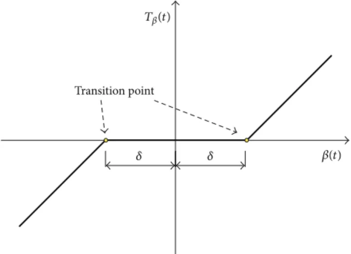
Transition point

�(t)

T�(t)

� �

Figure 2: Freeplay nonlinearity.

2. Aeroelastic System with Freeplay

he typical section airfoil shown inFigure 1with a trailing edge control surface is normally used to represent an aeroe-lastic system with three degrees of freedom that includes pitch�(�), plungeℎ(�), and control surface rotation�(�). his modeling was previously proposed in [22]. he structural properties of this system are represented by the springs ��, �ℎ, and��, structural damping, and inertial properties.

heodorsen theory is used to compute the aerodynamic forces; however, the same control strategy could be adopted for other aerodynamic theories [22,23].

he nonlinear discontinuity (freeplay) is considered to occur in the control surface spring�_�. So that the equation of motion for this system can be represented by

Mü(�) +Du̇(�) +F(K,u, �) = �Qu(�) +B_��u_�(�) , (1)

where M and D are, respectively, the structural mass and damping matrices,Qis a matrix of aerodynamic coeicients that depend on the airfoil geometry,� = (1/2)��2 is the dynamic pressure, and � is the air density and � is the airspeed.B_�� is a matrix of input (forces or moments). he vectoru(�) = {ℎ(�) �(�) �(�)}�represents the physical dis-placements andu_�(�)is the control force. he vectorF rep-resents the elastic restoring moment which depends on the control surface restoring moment�_�(�)shown inFigure 2.

By considering a freeplay amplitude of 2�, the elastic restoring moment can be written as

F(K,u, �) = {�_ℎ(�) �_�(�) �_�(�)}�such that

�ℎ(�) = �ℎℎ (�) ,

��(�) = �� (�) ,

��(�) = 0 if ��(�)�� ≤ �,

��(�) = ��[� (�) − �] if ��(�)�� > �.

(3)

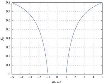
he expressions in (2) are rearranged in a matrix form and the nonlinear function�nlis introduced such that the stifness is deined as a nonlinear structural stifness matrixK_nlgiven by

K_nl= [ [

�ℎ 0 0

0 �� 0

0 0 ��

] ]�⇒

F(K,u, �) =K_nlu(�) , (3)

where

�nl= 0 if ��(�)�� ≤ �,

�nl= 1 − �_{� (�)} if ��(�)�� > �.

(4)

2.1. Representation in State Space Form. In order to obtain a nonlinear state space model, a rational function is used to write the aerodynamic forces in time domain. Jones in 1940 solved this problem using a rational function approximation to approximate unsteady aerodynamic loads for the typical section [24].

Ater Jones’ work, diferent formulations have been used to approximate generalized aerodynamic forces for arbitrary motion, as, for instance, the approach based on Chebyshev’s polynomials introduced by Dinu and colleagues with focus on aeroservoelasticity [25]. Karpel proposes the Minimum-State method with accuracy per model order superior to previous works, but it is more complicated and computing-time consuming because it involves nonlinear problems [26]. Vepa proposes a numerical technique based on Pad`e approx-imation and according to the author the main advantage of this method is that it can be generalized to three-dimensional liting surfaces [27]. Recently, Biskri and colleagues present a very interesting method based on a combination of the Least Squares (or Roger’s approach) and Minimum-State methods, of which the main idea is to minimize the number of lag terms without passing through a long iterative algorithm [28].

In this paper Roger’s approach is used. his approxi-mation involves identifying every matrix Q_� shown in (5) using a Least Square algorithm as proposed by Roger [29] and summarized in [30]. he approximation contains a polynomial part representing the forces on the typical section acting directly connected to the displacementsu(�)and their irst and second derivatives. Also, this equation has a rational part representing the inluence of the wake acting on the section with a time delay. Consider

Q(�) ≈ [ [

2

∑

�=0

Q_��( ��)

�

+

�lag

∑

�=1

Q_(�+2)( �

� + (�/�) ��)]_]u(�) ,

(5)

where�is the Laplace variable,�lagis the number of lag terms, �� is the �th lag parameter (� = 1, . . . , �lag), and� is the aerodynamic semichord.

Substituting (5) into (1) and considering (3) it is possible to write the equation of motion for the aeroelastic system in state space format:

̇

x(�) =A_nlx(�) +Bu_�(�) , y(�) =Cx(�) , (6)

wherex(�) = { ̇u(�) u(�) u_�(�)}�is the state vector andu_�(�) are states of lags required for the approximation of matrixQ. he matrix of outputsC= [CV C� C�]has dimension2� × �(2 + �lag), whereCV andC� are, respectively, the velocity and displacement output matrices and the submatrixC_�has only zeros to complete the matrix dimension, and�is the number of degrees of freedom. MatrixA_nlis presented in the following form:

A_nl

= [[ [[ [[ [[ [[ [

−M−1_� D_� −M−1_� K_�(nl) �M−1_� Q3 ⋅ ⋅ ⋅ �M−1_� Q(2+�lag)

I 0 0 ⋅ ⋅ ⋅ 0

I 0 (−��)�₁I 0 ⋅ ⋅ ⋅

..

. ... 0 d ⋅ ⋅ ⋅

I 0 ... ⋅ ⋅ ⋅ (−��)�_�_lagI

]] ]] ]] ]] ]] ] ,

(7)

where

M_� =M− �( ��)

2

Q₂, D_� =D− � ( ��)Q₁,

K_�(nl)=Knl− �Q0, B= [M−1_� B�� 0]

�_,

(8)

whereM_�andD_�are, respectively, the aeroelastic mass and damping matrices,K_�(_nl₎is the nonlinear aeroelastic stifness matrix,Bis the input matrix,Iis an identity matrix, and0is a matrix of zeros with appropriated dimension.

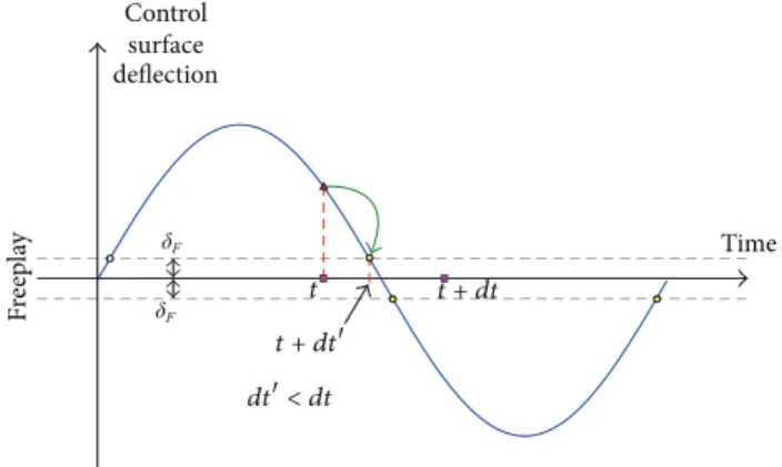
2.2. Time Integration. To calculate the time response of the system with freeplay a modiied 4th order Runge-Kutta algorithm using H´enon method is used. H´enon method is necessary in order to identify changes in the stifness due to the freeplay. his approach is used to minimize integration errors mainly with respect to the phase shits.

(4)

3. Development of Fuzzy

Takagi-Sugeno Controller

A fuzzy model uses rules, which are linguistic IF-THEN statements involving fuzzy sets, fuzzy logic, and fuzzy infer-ence. hese rules play a key role in representing expert control/modeling knowledge and experience and in linking the input variables of fuzzy controllers/models to output variable (or variables). To explain the procedure, consider the open loop nonlinear aeroelastic system described in following form:

̇�

�(�) = �

∑

�=1��(

x(�)) �_�(�) , (9)

whereu_�= 0,� = �(2 + �lag),� = 1, . . . , �, and��(x(�)) = �� represents the�th nonlinear function, where� = 1, . . . , �nl≤ �2_.

he nonlinear system described by (9) can be represented by the Takagi-Sugeno model using the following rule:

Rule�:

if�₁(�) is�_�1 and. . .and�_�(�) is �_��

henẋ(�) =A_�x(�) , y(�) =Cx(�) , � = 1, . . . , �, (10)

where�_��is the fuzzy set and�is the number of model rules; �1(�), . . . , ��(�)are known premise variables that in general

may be functions of the state variables, external disturbances, and/or times. Each linear model represented byA_�is called a subsystem [32].

Taniguchi et al. [33] present a simple method to identify the subsystems. he basic idea is to write each nonlinear function�_�as a linear combination of its maximum�_�maxand minimum�_�minvalues both given, respectively, by

�max

� = max[��(x(�))] ,

�min

� = min[��(x(�))] .

(11)

From these maximum and minimum values, each non-linear function can be represented by

��(x(�)) = [�min� (x(�))] �

min

� + [�

max

� (x(�))] �

max

� , (12)

where

0 ≤ �min

� (x(�)) , �

max

� (x(�)) ≤ 1,

�min

� (x(�)) + �

max

� (x(�)) = 1,

�min

� (x(�)) = [��(

x(�)) − �_�max] [�min

� − ��max] then,

�max

� (x(�)) = 1 − �

min

� (x(�)) .

(13)

If[�min_� (x(�))+�_�max(x(�)) = 1],∀� = 1, . . . , �nl, then each nonlinear function can be conveniently written as

��(x(�))

= ∏�nl

�=1,� ̸= �{�

min

� (x(�)) + �max� (x(�))}

× {[�min

� (x(�))] �

min

� + [�

max

� (x(�))] �

max

� } ,

(14)

or

��(x(�)) =

�1

∑

�=1��(

x(�)) �_�min+

(2�nl₎

∑

�=�1+1

��(x(�)) ��max, (15)

where�₁= 2(�nl−1)_and�

�(x(�))is given by

��(x(�)) =

�nl

∏

�=1�

(⋅) � (x(�)) ,

2�nl

∑

�=1��(

x(�)) = 1, (16)

and the superscript(⋅) indicates the combination between maximum and minimum values for each �th function �(⋅)

� (x(�)).

Considering thatAnl = Anl(�1, �2, . . . , ��nl)and substi-tuting each�_� according to (15), the nonlinear equation of motion (17) is rewritten ater some rearrangement as

̇

x(�) = (

2�nl

∑

�=1��(

x(�))A_�)x(�) + (

2�nl

∑

�=1��(

x(�))B_�)u_�(�) ,

(17)

where each linear matrixA_�is the original nonlinear matrix at which the�nlfunctions��are substituted by the combination of maximum and minimum values�_�maxand�_�min. In this case B_� =B∀�.

Particularly for the typical section including freeplay nonlinearity, there are three nonlinear functions(�nl = 3) into the matrixAnland they are given by

�1= �nl(1,6)= −M−1�(1,3)[��nl− �0.5�2Q0(1,3)] ,

�2= �nl(2,6)= −M−1_�(2,3)[��nl− �0.5�2Q0(2,3)] ,

�3= �nl(3,6)= −M−1�(3,3)[��nl− �0.5�2Q0(3,3)] ,

(18)

(5)

0 0.1 0.2 0.3 0.4 0.5 0.6 0.7 0.8

fnl

−5 −4 −3 −2 −1 0 1 2 3 4 5

�(t)/�

Figure 3: he nonlinear function�_nl represented in a particular range of�(�).

0 5 10 15

0 2 4 6 8 10 12 14 16

F

req

uenc

y (H

z)

Airspeed (m/s)

Control surface delection

Plunge mode Pitch mode

V-fdiagram: typical section

Figure 4: Linear lutter analysis:�-�diagram.

3.1. Closed-Loop Takagi-Sugeno Controller. In this section a feedback control strategy is used to control the amplitude of oscillation in the control surface. he feedback force is obtained by applying a feedback gain to the state systems states, such that the control inputs are given by u_�(�) = −Gx(�), whereGis the feedback gain matrix. he feedback gain is calculated using linear matrix inequality to solve Lyapunov’s function for stability, in this case

̇

x(�) = [ [

2�nl

∑

�=1��(

x(�)) (A_�−B_�G)] ]

x(�) , (19)

̇�

�= (

2�nl

∑

�=1��(

x(�)) [A_�−B_�G]x(�))

�

Px(�)

+x(�)�P(

2�nl

∑

�=1��(

x(�)) [A_�−B_�G]x(�)) < 0, (20)

0 5 10 15

Airspeed (m/s)

D

am

p

in

g ra

ti

o

Pitch mode

Control surface delection

Plunge mode

0.15

0.1

0.05

0

−0.05

−0.1

−0.15

−0.2

−0.25

−0.3

−0.35

V-gdiagram: typical section

12.7m/s

Figure 5: Linear lutter analysis:�-�diagram.

Table 1: Physical and geometric properties of the 2D airfoil.

Parameter Value

Semichord—� 0.15 m

Airfoil mass—� 5.0 kg

Air density—� 1.225 kg/m3

� 0.6%

� −0.4%

�� 0.2m/m

�� (6.25 × 10−3)−1/2m/m

�� 0.0125m/m

�� (0.25)−1/2m/m

Plunge frequency—�_ℎ 3.0 Hz

Pitch frequency—�_� 4.5 Hz

Control surface delection—�_� 12.0 Hz

Parameters of lag—�_�(� = 1, . . . , 4) 0.2, 1.2, 1.6, 1.8

Reduced frequency—� [0.1, 2.0],Δ� = 0.1

where�_� = x�Pxis the Lyapunov function. he stability of this system is assured if there is a positive-deinite matrix P such that the inequality of (20) is true. Ater some rearrangement this equation can be rewritten such as [32]

x�(�)

2�nl

∑

�=1��(

x(�))

× [(A_�−B_�G)�P+P(A_�−B_�G)]x(�) < 0, (21)

and inally, the solution of this inequality is equivalent to the solution of all the following inequalities satisied simultane-ously [34]:

(6)

0 2 4 6 8 10 12 14 0.5

1 1.5 2 2.5 3

Airspeed (m/s)

L

C

O a

m

p

li

tude (deg)

Initial conditions

Linear lutter boundary

Freeplay amplitude� = 0.4∘

Figure 6: LCO prediction for|�| = 0.4∘.

0 2 4 6 8 10 12 14

0.5 1 1.5 2 2.5 3 3.5 4

Airspeed (m/s)

L

C

O a

m

p

li

tude (deg)

Initial conditions

Freeplay amplitude� = 0.6∘

Figure 7: LCO prediction for|�| = 0.6∘.

Inequality (22) is not linear: then considering X = P−1, G_� = GX, it is possible to write the following linear matrix inequality:

XA�_� −G�_�B�_� +A_�X−B_�G_�< 0 � = 1, . . . , 2�nl

such that G=G_�X−1.

(23)

Although the control gainG has been computed using inequality (23), the required control forceu_�(�) can exceed desired limits. In this case, the control gain is multiplied by a

0 0.1 0.2 0.3 0.4 0.5 0.6 0.7 0.8 0.9 1

0 2 4 6 8 10 12 14

Air

sp

eed (m/s)

Normalized linear equivalent stiffness

keq/k�

Figure 8: Linear equivalent stifness from the HBM.

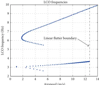
0 2 4 6 8 10 12 14

2 3 4 5 6 7 8 9 10

L

C

O f

req

uenc

y (H

z)

Airspeed (m/s) LCO frequencies

Figure 9: LCO frequencies obtained from the HBM.

constant�between the interval[0 1], conveniently adjusted during the control design. he control force is rewritten as

u_�(�) = �u_�(�) or u_�(�) = −�Gx(�) . (24)

4. Numerical Application

To illustrate the method, numerical simulations were per-formed using the three degrees of freedom airfoil section for which the equations of motion are presented by heodorsen et al. in [23]. he structural mass, stifness, and aerodynamic forces matrices can be found in [17,22,35].

(7)

−100

−120

−140

−25 −20 −15 −10 −5 0 5 10 15 20 25

500

0

−500

0

−5000

−10000 f1

f2

f3

fk

�/�

−25 −20 −15 −10 −5 0 5 10 15 20 25

�/�

−25 −20 −15 −10 −5 0 5 10 15 20 25

�/�

gmink fkmin+ gmaxk fkmax

Figure 10: Values of�_�: actual versus computed using TS approach.

0 2 4 6 8 10 12 14 16 18 20

Time (s)

0 10 20 30 40 50 60 70 80 90 100

Frequency (Hz)

Uncontrolled

~3.7 ~48

Uncontrolled Controlled

∼15 1

0.5

0

−0.5

−1

�(

t)

−20

−40 −60

−80 −100

|�

|

(dB)

Control surface rotation,�F= 0.4∘

±�F

Figure 11: Case1: control surface rotation (|�| = 0.4∘ and� =

12.5m/s).

LCO amplitudes. Diferent researchers have used HBM meth-ods to study limit cycles oscillations in aeroelastic systems, as shown in [3,6,36,37].

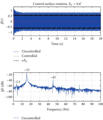
0 2 4 6 8 10 12 14 16 18 20

Time (s)

0 10 20 30 40 50 60 70 80 90 100

Frequency (Hz) ~3.5

~15

~45

1

0.5 0 −0.5 −1

−20 −40 −60 −80 −100

�(

t)

|�

|

(dB)

Uncontrolled

±�F

12.5m/s).

4.1. Linear Flutter Boundary. Figure 1illustrates the model and its physical and geometric properties are presented in Table 1. Figures4and5show, respectively, the classical�-� and�-�diagrams for the linear lutter solution. According to these results lutter speed is equal to 12.7 m/s.

4.2. LCO Preliminary Predictions. Ater the preliminary lin-ear analysis to identify the lutter boundary, the irst order HBM was used to predict the LCO amplitudes. he results shown in Figures6 and 7were obtained by extracting the eigenvalues from the matrixAnl deined for diferent values of equivalent stifness�eq, that is, the control surface stifness assuming values from zero to �_�. he values of�eq/�� are shown inFigure 8, where the nonlinear function�nlassumed a unitary value and the control forceu_�(�) = 0. he HBM also provided an estimate for the irst harmonic of the system response according toFigure 9.

4.3. Controller Design. Using the methodology described in Section 4, three nonlinear functions were used to describe the aeroelastic system with freeplay (�_�,� = 1, 2, 3). hese functions were computed assuming the maximum oscillation amplitude equal to ive degrees; that is,−5∘ ≤ �(�) ≤ 5∘. Figure 10shows a comparison between their actual values and computed values by (12).

(8)

0.05

0

−0.05

0.05

0

−0.05

−2 0 2

̇_h(t)

̇

�(

t)

̇

�(

t)

̇_�(t)

−5 0 5 −0.02

−0.2

0 0

0.02 0.2

−0.1 0 0.1

h(t) uncontrolled �(t) uncontrolled �(t) uncontrolled

h(t) controlled �(t) controlled �(t) controlled

×10−3 ×10−3

×10−4

×10−6

−2 0 2

−5 0 5 −5 0 5

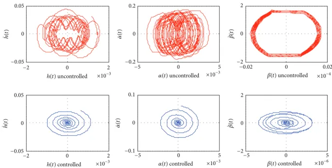
Figure 13: Case1: phase plan (|�| = 0.4∘and� = 12.5m/s).

0.05

0

−0.05

0.05

0

−0.05

−5 0 5

−2 0 2

̇_h(t)

̇

�(

t)

̇

�(

t)

̇_�(t)

−5 0 5 −0.02

−0.2

0 0

0.02 0.2

−0.1 0 0.1

�(t) uncontrolled

h(t) uncontrolled �(t) uncontrolled

×10−3 ×10−3

×10−3 _×10−3

×10−4

×10−6

−2 0 2

−5 0 5 −5 0 5

Figure 14: Case: phase plan (|�| = 0.6∘and� = 12.5m/s).

functions, such that

A₁=A(�₁max, �₂min, �₃min) , A₂=A(�₁max, �₂max, �₃min) ,

A₃=A(�₁min, �₂max, �₃min) , A₄=A(�₁min, �₂min, �₃min) ,

A₅=A(�₁max, �₂min, �₃max) , A₆=A(�₁max, �₂max, �₃max) ,

A₇=A(�₁min, �₂max, �₃max) , A₈=A(�₁min, �₂min, �₃max) . (25)

he results shown in this section were obtained consider-ing two diferent freeplay amplitudes and a time step equal

to 0.001 seconds. To compute the control gain, a column input matrix was used to represent an actuator applying force on the control surface (B_�� = {0 0 1}�). Also, it was considered that the parameter�is equal to1.0for all cases. However, in particular for experimental applications where limitations exist on the actuator force, the parameter�can be conveniently chosen between ]0, 1[.

For the cases in which the freeplay amplitude was|�| = 0.4∘_{, the initial conditions were}_{�(0) = 0.9}∘_and_2.5∘_{. Similarly,}

(9)

0 1 2 3 4 5 6 7 8 9 Time (s)

4

3

2

1

0

−1

−2

−3

−4

�(

t)

±�F

13.1m/s).

�(0) = 1.3∘_and_3.5∘_{. hese values were deined based on the}

results obtained from the HBM, as discussed inSection 4.2. Two diferent conditions of airspeed were considered to demonstrate the method. Diferent controllers were designed for each case. In irst case was chosen a condition of stable limit cycle for each freeplay amplitude. In the second one, unstable limit cycles were chosen in order to evaluate the efectiveness of the approach. Consider if all neighboring trajectories approach the LCO, it is stable; otherwise, the LCO is unstable. Deinitions and a detailed discussion about stable and unstable limit cycles can be found in [38].

Case 1 (stable LCO). In the irst case � = 12.5m/s was considered for both freeplay amplitudes. Figures11 and 12 show that the uncontrolled system response exhibits a limit cycle oscillation with irst harmonic around 3.7 Hertz and amplitude approximately equal to 1 degree. It is possible to note in those igures that although the irst order HBM cannot predict, the system response exhibits a dominant component around 15 Hertz. In addition, the plunge and pitch degrees of freedom behavior can be observed in the phase plan shown in Figures 13 and 14. In these cases of stable LCOs the designed controllers were able to suppress the limit cycles. he appendix presents details involved to compute the Fourier transform when H´enon’s technique is used for the time integration process.

Case 2 (unstable LCO). In this case was considered � = 13.1m/s for both freeplay amplitudes. Figures15and16show that the uncontrolled system response exhibits an unstable limit cycle. However, the controller gains computed using the proposed approach are able to suppress those nonlinear responses. To improve the comprehension,Figure 17shows a

0 1 2 3 4 5 6 7 8 9

Time (s)

6

4

2

0

−2

−4

−6

�(

t)

±�F

13.1m/s).

0 0.02 0.04 0.06 0.08 0.1 0.12 0.14 0.16 0.18 0.2

Time (s)

3

2

1

0

−1

−2

−3

�(

t)

±�F

Figure 17: Case 2: zoom selection area for the control surface rotation (|�| = 0.6∘and� = 13.1m/s).

zoom selection area for the control surface rotation consider-ing the second freeplay amplitude.

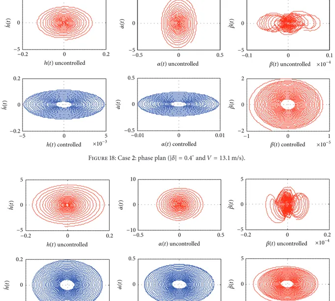
For this second case the plunge and pitch degrees of freedom behavior can be observed in the phase plan shown in Figures18and19. Finally,Figure 20shows the control force for�_� = 0.6∘and similar results were obtained for the other cases. Note that the parameter� < 1.0can be chosen in order to decrease the required control force mainly for the irst time steps.

5. Conclusions

(10)

5

0

0 −5

−5

5

0

−5

5

0

−5

0.5

0

−0.5

̇_h(t)

̇

�(

t)

̇

�(

t)

̇_�(t)

−0.01 0 0.01

�(t) uncontrolled

h(t) uncontrolled _{�(t) uncontrolled}

h(t) controlled ×10−3 �(t) controlled �(t) controlled ×10−5

×10−4

−2 0 2

−0.2 0 0.2

−1 0 1

−0.2 0 0.2 −0.5 0 0.5 _−0.1 ₀ _0.1

5

0.01

0

0 −5

−0.01

10

0

−10

5

0

−5

0.5

0

−0.5

̇_h(t)

̇

�(

t)

̇

�(

t)

̇_�(t)

5

0

−5

̇_�(t)

−0.02 0 0.02

�(t) uncontrolled

h(t) uncontrolled �(t) uncontrolled

×10−4

×10−5

−0.2 0 0.2

−2 0 2

−0.2 0 0.2 −0.5 0 0.5 −0.2 0 0.2

freeplay. he idea was to use the fuzzy Takagi-Sugeno mod-eling to describe the nonlinear aeroelastic system through linear matrix inequalities. he closed-loop problem was written using a convex space and a linear control force was computed using convex optimization. A linear lutter analysis was performed to identify the lutter boundary. Also, the irst order harmonic balance method was solved to predict the limit cycle oscillation envelope. Ater these irst predictions two freeplay amplitudes were deined and two airspeeds were chosen to demonstrate stable and unstable limit cycles. Finally, numerical simulations presented diferent nonlinear aeroelastic responses comparing the controlled and uncon-trolled system. he results show that fuzzy TS modeling is an eicient tool for solving this kind of problem.

Appendix

(11)

0 0.1 0.2 0.3 0.4 0.5 0.6 0.7 0.8 0.9 Time (s)

Control force

50

0

−50

−100

g

uc

(t

)

Figure 20: Case2: control force (|�| = 0.6∘and� = 13.1m/s).

Control

surface deﬂection

Time

Fre

ep

lay

t t + dt

t + dt󳰀

dt󳰀< dt

Figure 21: Illustrative scheme of integration process using H´enon’s technique.

Conflict of Interests

he authors declare that the research was conducted in the absence of any commercial or inancial relationships that could be construed as a potential conlict of interests.

References

[1] M. D. Conner, D. M. Tang, E. H. Dowell, and L. N. Virgin, “Non-linear behavior of a typical airfoil section with control surface freeplay: a numerical and experimental study,”Journal of Fluids and Structures, vol. 11, no. 1, pp. 89–109, 1997.

[2] M. D. Conner, L. N. Virgin, and E. H. Dowell, “Accurate numer-ical integration of state-space models for aeroelastic systems with free play,”AIAA Journal, vol. 34, no. 10, pp. 2202–2205, 1996.

[3] D. Tang, E. H. Dowell, and L. N. Virgin, “Limit cycle behavior of an airfoil with a control surface,” Journal of Fluids and Structures, vol. 12, no. 7, pp. 839–858, 1998.

[4] N. Krylof and N. Bogoliubof,Introduction to Nonlinear Mech-anics, Princeton University Press Books, 1947.

[5] H. Y. Hu, E. H. Dowell, and L. N. Virgin, “Stability estimation of high dimensional vibrating systems under state delay feedback control,”Journal of Sound and Vibration, vol. 214, no. 3, pp. 497– 511, 1998.

[6] G. Dimitriadis, Investigation of nonlinear aeroelastic system [Ph.D. thesis], University of Manchester, 1999.

[7] S. T. Trickley, L. N. Virgin, and E. H. Dowell, “he stability of limit-cycle oscillations in a nonlinear aeroelastic system,” Proceedings of the Royal Society A: Mathematical, Physical and Engineering Sciences, vol. 458, no. 2025, pp. 2203–2226, 2002. [8] L. Liu and E. H. Dowell, “Harmonic balance approach for an

airfoil with a freeplay control surface,”AIAA Journal, vol. 43, no. 4, pp. 802–815, 2005.

[9] D. Kholodar and M. Dickinson, “Aileron freepaly,” in Proceed-ings of the International Forum of Aeroelasticity and Structural Dynamics (IFASD ’10), 2010.

[10] W. D. Anderson and S. Mortara, “Maximum control surface freeplay, design and light testing approach on the F-22,” in Proceedings of the 48th AIAA/ASME/ASCE/AHS/ASC Structures, Structural Dynamics, and Materials Conference, AIAA Paper 07-1767, pp. 767–778, April 2007.

[11] A. Abdelkei, R. Vasconcellos, F. D. Marques, and M. R. Hajj, “Modeling and identiication of freeplay nonlinearity,”Journal of Sound and Vibration, vol. 331, no. 8, pp. 1898–1907, 2012. [12] R. Vasconcellos, A. Abdelkei, F. D. Marques, and M. R. Hajj,

“Representation and analysis of control surface freeplay nonlin-earity,”Journal of Fluids and Structures, vol. 31, pp. 79–91, 2012. [13] H. Guo and Y. Chen, “Dynamic analysis of two-degree-of-freedom airfoil with freeplay and cubic nonlinearities in super-sonic low,”Applied Mathematics and Mechanics, vol. 33, no. 1, pp. 1–14, 2012.

[14] A. J. Kurdila, T. W. Strganac, J. L. Junkins, J. Ko, and M. R. Akella, “Nonlinear control methods for high-energy limit-cycle oscillations,”Journal of Guidance, Control, and Dynamics, vol. 24, no. 1, pp. 185–192, 2001.

[15] T. W. Strganac, J. Ko, D. E. hompson, and A. J. Kurdila, “Iden-tiication and control of limit cycle oscillations in aeroelastic systems,”Journal of Guidance, Control, and Dynamics, vol. 23, no. 6, pp. 1127–1133, 2000.

[16] G. Platanitis and T. W. Strganac, “Control of a nonlinear wing section using leading-and trailing-edge surfaces,” Journal of Guidance, Control, and Dynamics, vol. 27, no. 1, pp. 52–58, 2004. [17] D. Li, S. Guo, and J. Xiang, “Aeroelastic dynamic response and control of an airfoil section with control surface nonlinearities,” Journal of Sound and Vibration, vol. 329, no. 22, pp. 4756–4771, 2010.

[18] R. B. Alstrom, P. Marzocca, E. Bollt, and G. Ahmadi, “Con-trolling chaotic motions of a nonlinear aeroelastic system using adaptive control augmented with time delay,” in Proceedings of the AIAA Guidance, Navigation, and Control Conference, Number 8146, August 2010.

[19] S. da Silva and V. L. J´unior, “Active lutter suppression in a 2-D airfoil using linear matrix inequalities techniques,”Journal of the Brazilian Society of Mechanical Sciences and Engineering, vol. 28, no. 1, pp. 84–93, 2006.

[20] C. Gao, G. Duan, and C. Jiang, “Robust controller design for active lutter suppression of a two-dimensional airfoil,” Nonlin-ear Dynamics and Systems heory, vol. 9, no. 3, pp. 287–299, 2009.

(12)

[22] T. heodorsen, “General theory of aerodynamic instability and the mechanism of lutter,” NACA Report 496, National Advisory Committee for Aeronautics—NACA, 1935.

[23] T. heodorsen, I. E. Garrick, and NACA Langley Research Center,Mechanism of Flutter a heoretical and Experimental Investigation of the Flutter Problem, National Advisory Commit-tee for Aeronautics, 1940.

[24] R. T. Jones, “he unsteady lit of a wing of inite aspect ratio,” Tech. Rep. 681, National Advisory Committee for Aeronautics— NACA, 1940.

[25] A. D. Dinu, R. M. Botez, and I. Cotoi, “Aerodynamic forces approximations using the chebyshev method for closed-loop aeroservoelasticity studies,” Canadian Aeronautics and Space Journal, vol. 51, no. 4, pp. 167–175, 2005.

[26] M. Karpel, “Design for active and passive lutter suppression and gust alleviation,” TR 3482, National Aeronautics and Space Administration—NASA, 1981.

[27] R. Vepa, “Finite state modeling of aeroelastic systems,” Contrac-tor Report CR 2779, NASA—National Aeronautics and Space Administration, 1977.

[28] D. Biskri, R. M. Botez, N. Stathopoulos, S. h´erien, A. Rathe, and M. Dickinson, “New mixed method for unsteady aero-dynamic force approximations for aeroservoelasticity studies,” Journal of Aircrat, vol. 43, no. 5, pp. 1538–1542, 2006.

[29] K. L. Roger, “Airplane math modelling methods for active control design,”AGARD Conference Proceeding, vol. 9, pp. 4. 1– 4. 11, 1977.

[30] I. Arbel, “An analytical technique for predicting the charac-teristics of a lexible wing equipped with an active lutter-suppression system and comparison with wind-tunnel data,” TP 1367, National Aeronautical and Space Administration—NASA, 1979.

[31] J. Awrejcewicz and P. Olejnik, “Numerical analysis of self-excited by friction chaotic oscillations in two-degrees-of-freedom system using exact henon method,”Machine Dynamics Problems, vol. 26, no. 4, pp. 9–20, 2002.

[32] K. Tanaka and H. O. Wang, Fuzzy Control Systems Design and Analysis: A Linear Matrix Inequality Approach, Wiley-Interscience, 2001.

[33] T. Taniguchi, K. Tanaka, H. Ohtake, and H. O. Wang, “Model construction, rule reduction, and robust compensation for generalized form of Takagi-Sugeno fuzzy systems,”IEEE Trans-actions on Fuzzy Systems, vol. 9, no. 4, pp. 525–537, 2001. [34] B. R. Barmish, “Necessary and suicient conditions for

qua-dratic stabilizability of an uncertain system,”Journal of Opti-mization heory and Applications, vol. 46, no. 4, pp. 399–408, 1985.

[35] D. Dessi and F. Mastroddi, “Limit-cycle stability reversal via singular perturbation and wing-lap lutter,”Journal of Fluids and Structures, vol. 19, no. 6, pp. 765–783, 2004.

[36] S. F. Shen, “An approximate analysis of nonlinear lutter prob-lem,”Journal of the Aerospace Sciences, vol. 26, no. 1, pp. 25–32, 1959.

[37] G. A. Vio and J. E. Cooper, “Limit cycle oscillation prediction for aeroelastic systems with discrete bilinear stifness,” Interna-tional Journal of Applied Mathematics and Mechanics, vol. 3, pp. 100–119, 2005.

(13)