2007, Vol. 3 (2), p. 70‐78.
Power Estimation in Multivariate Analysis of Variance
Sylvain Chartier University of Ottawa Institut Philippe Pinel de Montréal
Jean‐François Allaire Institut Philippe Pinel de Montréal
Power is often overlooked in designing multivariate studies for the simple reason that it is believed to be too complicated. In this paper, it is shown that power estimation in multivariate analysis of variance (MANOVA) can be approximated using a F distribution for the three popular statistics (Hotelling‐Lawley trace, Pillai‐Bartlett trace, Wilk`s likelihood ratio). Consequently, the same procedure, as in any statistical test, can be used: computation of the critical F value, computation of the noncentral parameter (as a function of the effect size) and finally estimation of power using a noncentral F distribution. Various numerical examples are provided which help to understand and to apply the method. Problems related to post hoc power estimation are discussed.
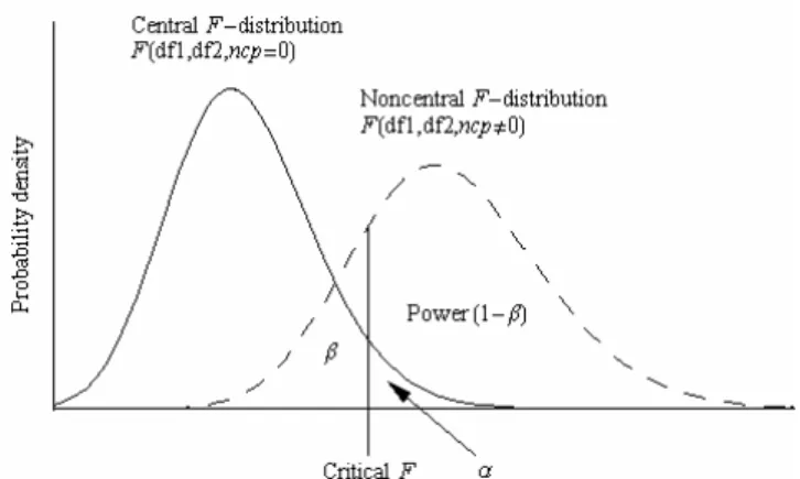
Because it is a central tool in the design of any study, statistical power is introduced in all statistics textbooks. Power reflects the probability of rejecting a false null hypothesis (Figure 1). However, power is often overlooked when designing a multivariate study for the simple reason that it is believed to be too difficult to estimate. Because power is related to sample size, the later must be adjusted accordingly. If the sample size is too small, the study will not be sensitive enough and if the sample size is too big, the study will waste valuable resources. Consequently, estimating power is essential and the choice of power depends on the research question, measurement, design and analysis plan (Cohen, 1988; Muller, LaVange, Landesman Ramey, & Ramey, 1992). In this paper, it is shown that power estimation in multivariate analysis of variance (MANOVA) is a direct generalization of its estimation in univariate analysis of variance (ANOVA) through the general linear model (GLM).
Figure 1. Power and errors illustrative concepts
Power can be estimated before the study or after the study. The first situation will be referred to as prospective (or a priori) power estimation and the second as
The authors
are grateful to an anonymous reviewer for hishelp in preparing this article
retrospective (post hoc) power estimation. Power is important for design, not analysis (Lenth, 2001). Since studies can be statistically significant yet clinically insignificant; time should be spent on what is clinically significant in respect to the study hypothesis. Statistics are used to help in reaching that goal, not the other way around (Lenth, 2001). Post hoc power estimation may be useful for a pilot study where procedures are established and the obtained variance estimates are used for determining sample size or effect size for future experiments. The general procedure for power estimation is:
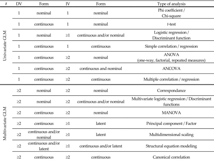
Table 1 Univariate and multivariate representations of the GLM
# DV Form IV Form Type of analysis
1 nominal 1 nominal Phi coefficient / Chi‐square
1 continuous 1 nominal t‐test
1 nominal ≥1 continuous and/or nominal Discriminant function Logistic regression /
1 continuous 1 continuous Simple correlation / regression
1 continuous ≥2 nominal (one‐way, factorial, repeated measures) ANOVA
1 continuous ≥2 continuous and nominal ANCOVA
U
n
iv
ariat
e
GL
M
1 continuous ≥2 continuous Multiple correlation / regression
≥2 nominal ≥2 nominal Correspondance
≥2 nominal ≥2 continuous and/or nominal Multivariate logistic regression / Discriminant functions
≥2 continuous ≥2 nominal MANOVA
≥2 continuous ≥1 latent Principal component / Factor
≥2 continuous and/or nominal ≥1 latent Multidimensional scaling
≥2 continuous and/or latent ≥1 continuous and/or latent Structural equation modeling
Mult
iv
ariat
e
GL
M
≥2 continuous ≥2 continuous Canonical correlation
2‐ Compute the noncentral parameter ncp (as a function of the effect size)
3‐ Compute the power using the noncentral F distribution
Whatever the design (regression, ANOVA, MANOVA, etc.), the same procedure is always applied. Using this procedure, the sample size required to reach a given power can be computed using the Mathematica function provided in Listing 2 (see the Numerical example III section).
Multivariate analysis of variance
When a research design contains two or more dependent variables there is two possible type of analysis: multiple univariate tests or one multivariate test. Performing multivariate analysis of variance (MAOVA) has many advantages (Baguley, 2004; Stevens, 1992). First, MANOVA does not have the problem of inflated overall type I error rate (α) that occurs when using multiple univariate tests. In addition, when multiple univariate tests are used, estimation of the type I error inflation is difficult since the multiple tests are not independents. Second, univariate tests ignore the correlations among the variables. On the other
hand, in multivariate tests, the correlation matrix (via the covariance) is directly incorporated into the analysis. Finally, since the groups are combined in the overall effect, multivariate tests are more powerful than multiple univariate tests; the same argument applies when choosing one ANOVA instead of multiple t tests.
In this paper, attention will be focus on MANOVA. MANOVA requires two or more categorical independent variables (predictors), just like in ANOVA. However, unlike ANOVA, it uses two or more dependent variables (criterions). MANOVA is thus employed to test the main and interaction effects on multiple dependent variables. Like any other linear statistics, Table 1 shows that MANOVA is part of the general linear model (GLM) and is in fact a special case of canonical correlation analysis (Thompson, 1984).
Listing 1. Mathematica function for power estimation
factor (βih) and/or their interaction (αβijh). This is described by the following
yijhr=μh+αih+βjh+αβijh+eijhr (1)
h = 1, 2, …, q; i = 1, 2, …, k; j = 1, 2, …, l; r = 1, 2, …, n.
With an appropriate coding matrix, it is possible to represent this situation in general linear term.
Y=XB+E (2)
where the matrix B contains the coefficients used in Equation 1, such that,
1 11 21 1 1 11 21 1 1 111 121 1 1 1
2 12 22 1 2 12 22 1 2 112 122 1 1 2
1 2 1 1 2 1 11
, , ,..., , , ,..., ,( ) ,( ) ,...,( ) , , ,..., , , ,..., ,( ) ,( ) ,...,( )
, , ,..., , , ,..., ,( ) ,(
μ α α α β β β αβ αβ αβ
μ α α α β β β αβ αβ αβ
μ α α α β β β αβ α
− − −
− − −
− −
=
#
k l k l
k l k
q q q k q q q l q q
B
T
12 1 1
) ,...,( )
β αβ − −
⎡ ⎢ ⎢ ⎢ ⎢
⎢⎣ q k l q⎦
− − l ⎤ ⎥ ⎥ ⎥ ⎥ ⎥
11 12 1
⎡ ⎤
⎢ ⎥
⎥
"
X represents the predictor matrix obtained from a coding matrix (see below), q is the number of dependant variables, k and l are the number of groups for treatment
α
andβ
respectively.The coding matrix X is not different from the one used in univariate analysis. This full matrix is constructed by building two coding matrices for each factor (α and β) and then multiplying each column of the first factor with each column of the second factor to give the interaction coding matrix (αβ). An example of effect coding is shown in Table 2. Although an effect coding matrix is used for full factorial analysis, any other type of coding (e.g. contrast, dummy) can be used as well as any kind of mixed coding (e.g. α: contrast; β: dummy). From the coding matrix in figure 2 the predictor matrix X is constructed as follows.
21 22 2
1 2 ⎢ = ⎢ ⎥ ⎢ ⎥ ⎢ ⎥ ⎣ ⎦ " # # % # " p p i
n n np
x x x
x x x
x x x
X (3)
where i ∈ {full (α, β and αβ); α; β; or αβ}, n is the total number of subject and p is the number of independent predictors. In the full factorial model p will be set to (k×l)‐1. Finally, the criterion matrix Y contains the observed data and is organized as follow:
(4)
where q the number of criterions (dependant variables). These two matrices can be concatenated into a single matrix
11 12 1
⎡ ⎤
⎢ ⎥
⎥
" q
y y y
11 12 1 11 12 1
21 22 2
1 2 ⎢ = ⎢ ⎥ ⎢ ⎥ ⎢ ⎥ ⎣ ⎦ " # # % # " q
n n nq
y y y
y y y
Y
21 22 2 21 22 2
1 2 1 2
⎡ ⎤ ⎢ ⎥ ⎢ ⎥ = ⎢ ⎥ ⎢ ⎥ ⎢ ⎥ ⎣ ⎦ " " # # % # # # % # " "
" p " q
p q
i
n n np n n nq
x x x y y y
x x x y y y
x x x y y y
M (5)
where, xij, represents the ith subject of jth predictor, yih represents the ith subject of the hth criterion, n the number of subjects per groups, p the number of predictor and q the number of criterion. In the case of the full model (Table 2) the sum of square and cross product (SSCP) matrix will be needed. The SSCP matrix is obtained by
T T T T (6)
( ) ( )
= Full Full− Full Full n
SSCP M M 1 M 1 M /
where 1 is defined as the vector in which all the elements are 1, and T denotes the matrix transposition operation. As a further optional processing, when the SSCP is divided by the corresponding degrees of freedom (n ‐ 1) then the variance/covariance matrix is obtained. Therefore, the SSCP is a convenient way to represent all information about variability in one matrix.
By partitioning the SSCP matrix correctly, the canonical correlation matrix, R, can be obtained. The SSCP must be divided in four sections named Spp, Spc, Scp, Scc which represents the sum of squares of the predictors alone, the sum of cross‐product between the predictors and the criterion, the sum of cross‐product between the criterion and the predictors (note that Scp = SpcT) and the sum of squares of Table 2 Effect coding matrix for two‐level factorial ANOVA
1
α
β
αβ
x
1 1 1 21 2 1 1 2 1 1
1 1 2 1 1 1 2 2 2
1 0
0
1
0
0
1
0
0
0 1
0
1
0
0
0
0
0
1 1
1 1
0
0
1
0
0
1 0
0
0
1
0
0
0
0
0 1
0
0
1
0
0
0
0
1 1
1
1
1
1
1
1
αβ
α β
α β
αβ
αβ
α β
+ − + − − + + − + − + −− −
−
−
− −
− − −
−
"
"
"
"
"
"
"
"
"
"
#
# # % # # # % #
#
# % #
"
"
"
"
"
"
"
"
"
#
# # % # # # % #
#
# % #
"
"
"
m m m m n
m m m m n m n m n mn
m
m n
x
xx
x x
Group x x
x
x
x
x
x
x
x
Table 3 Summary table of the m and i symbolic variables.
α
β
HLi
Type of analysis
(i)
αβ
α
β
PBi
Type of analysis (i)
αβ
α
β
Type of statistics (m)Wi analysis Type of
(i)
αβ
the criterion alone respectively This is summarized using: =⎡⎢ ⎤⎥ ⎢ ⎥ ⎣ ⎦ pp pc cp cc SSCPs
s
s
s
(7)The canonical correlation matrix can be obtained by the following matrix multiplication
= T −1 −1
pc pp pc cc
R S S S S (8)
From R, the error matrix (E) can be computed
E= −(I R S) cc (9)
The degree of freedom associated with the error is given by
dferr= − ×n k l (10)
The total variation is the sum of the various hypothesis variation add to the error variation, i.e. T=E+Hα+Hβ+Hαβ. Each matrix H is obtained by
T T 1 T (11)
( )−
=
i i i i i
H Y M M M M Y
where i ∈{α, β, αβ}; the full model is omitted when performing hypothesis testing. In univariate, the statistics used is based on the F‐ratio distribution.
2 2
2 1 (1 ) = − R df F
R df (12)
However, in MANOVA there is no unique statistic. Four statistics are commonly used: Hotelling‐Lawley trace (HL), Pillai‐Bartlett trace (PB), Wilk`s likelihood ratio (W) and Roy’s largest root (RLR). Those statistics can be obtained from Equations 9 and 11, as seen here.
The HL statistic is defined as
1
=1
=tr( −)=
∑
λs
i i
k
HL H E k (13)
where s = min(dfi, q), i represents the tested effect (i ∈{α, β, αβ}), dfi is the degree of freedom associated with the hypothesis under investigation (α, β or αβ) and λk is kth eigenvalue, i.e. the kth nonzero root of the following characteristic equation
H−λE =0 (14)
where |H‐λE| is the determinant of H‐λE. The PB statistic is defined as
1
=1
tr( ( ) )
1 λ λ − = + = +
∑
s ki i i
k k
PB H E H (15)
The W statistic is defined as 1 1 1 λ = = = +
∏
+ s ii k k
W E
E H (16)
Finally, the RLR statistic is defined as ( ) 1 ( λ ) λ = + k i k Max RLR
Max (17)
All the statistics are equivalent when s = 1. In general there is no exact formula for finding the associated p value except on
rare situations1. Nevertheless, a convenient and sufficient approximation exists for all but RLR (Muller et al., 1992). Since RLR is the least robust (Olson, 1974), attention will be focused on the first three statistics: HL, PB and W. These three statistics’ distributions are approximated using an F distribution which has the advantage of being simple to understand. The multivariate F‐ratio is function of their multivariate association coefficient. 2 2 2 1 ( ) ( ) (1 ) η η = − i i m i i m df m F m
df (18)
where df1 represents the numerator degree of freedom (df1 = q*dfi), df2(m) the denominator degree of freedom for each statistic m (m ∈ {HLi, PBi and Wi}) and
η
m2is the multivariate measure of association for each statistic m (see Table 3 for the detailed values of the symbolic indices used in Equation 18).
The multivariate measure of association for HL is given by
η2 =
+ i i HL i HL
HL s (19)
and its denominator df by
df2(HLi)=s df
(
err− − +q 1)
2The multivariate measure of association for PB is given by
(20)
η2 =
i
i PB
PB
s (21)
and its denominator df by
df2(PBi)=s df
(
err− +q s)
The multivariate measure of association for W is given by
(22)
2 1
1
η = − g
i
W Wi (23)
and its denominator df by
1
For example, Tatsuoka (1988) gives the exact formula for
Listing 2. Mathematica function for sample size estimation
1
2( ) 1
2
= + −
i
df
df W og (24)
where
and
( 1 ) / 2
= err− + − i
o df q df
(
) (
(
)
)
12
2 2 2
4 /
= i − i
g q df q +df2−5 .
Equation 23 (like Equations 19 and 21) are related with Cohen effect size f2 (Cohen, 1988) using the following equivalence
2 2
i 2
f 1
η η
= −
i i
W
W
(25)
The only missing information to obtain the power is the value of the noncentral parameter ncp. It is obtained by the following
2
2 2
1 2 i
( )
( ) ( ) f ( )
(1 )
η η
= = =
−
i i
m i
i i
m df m
ncp m df F m df m2 i (26)
Thus power can be estimated if an F‐value (a priori or observed) or a multivariate association coefficient
i
m
2
η
or aCohen’s i is given. Now that all the relevant information has been obtained following the general procedure previously described it is possible to find the estimated power
2
f
(
)
(
1 2)
( i)≈ −1 , , ( i) ,
Power m CDF NoncentralFdistribution df df ncp m Fcrit
(27)
Where Fcrit is given by the inverse of a central F‐distribution
1
(
)
(28)1 α, ,
−
= −
Fcrit CDF df df1 2
The Listing 1 shows a Mathematica function that evaluates the power given the numerator and denominator df, the multivariate association coefficient (
i
m
2
η
) and thetype‐I error (α); the default value is set to α = 0.05.
Numerical example I: Post hoc power
In this section, power estimations are computed for the weight losses data given by Table 5.5 of Morrison (1976) reproduced in Table 4. The two factors are the sex of the rats Table 4 Weight loss and time to complete a maze as a function of the sex of the rat and the type of drug ingested
Drug
A B C
Male
5, 6 5, 4 9, 9 7, 6
7, 6 7, 7 9, 12
6, 8
21, 15 14, 11 17, 12 12, 10
Female
7, 10 6, 6 9, 7 8, 10
10, 13 8, 7 7, 6 6, 9
and the type of drug administered (among three) resulting in 2×3 design (α = 2, β = 3). There were four rats of each sex assigned to each drug. Finally, weight losses in grams and the time to run the maze in second were observed; Therefore, there is two dependent variables (q = 2). Using Table 2 we construct the following coding matrix.
1 1 1 1 0 1 0
1 0 1 0 1
1 2 1 3 2 1 2 2 2 3
1 1 1 1 1
1 1 0 1 0
1 0 1 0 1
1 1 1 1 1
α β αβ
α β α β α β α β α β α β
− − − −
− −
− −
− − −
From this matrix, it is then possible to obtain the matrix M by assigning the corresponding row, and the corresponding criterion value, to each subject. For example, the first row [1, 1, 0, 1, 0] correspond to the “male” subjects that has received the “drug A”. There are four subjects that belong to this category. Therefore, this row will be repeated four times and each one of them will be aggregated with the corresponding subject scores on the two criterions (weight loss and time).
X Y
α β αβ
s1 1 1 0 1 0 5 6
s2 1 1 0 1 0 5 4
s3 1 1 0 1 0 9 9
s4 1 1 0 1 0 7 6
s5 1 0 1 0 1 7 6
s6 1 0 1 0 1 7 7
s7 1 0 1 0 1 9 12
s8 1 0 1 0 1 6 8
s9 1 ‐1 ‐1 ‐1 ‐1 21 15
s10 1 ‐1 ‐1 ‐1 ‐1 14 11
s11 1 ‐1 ‐1 ‐1 ‐1 17 12
M = s12 1 ‐1 ‐1 ‐1 ‐1 12 10
s13 ‐1 1 0 ‐1 0 7 10
s14 ‐1 1 0 ‐1 0 6 6
s15 ‐1 1 0 ‐1 0 9 7
s16 ‐1 1 0 ‐1 0 8 10
s17 ‐1 0 1 0 ‐1 10 13
s18 ‐1 0 1 0 ‐1 8 7
s19 ‐1 0 1 0 ‐1 7 6
s20 ‐1 0 1 0 ‐1 6 9
s21 ‐1 ‐1 ‐1 1 1 16 12
s22 ‐1 ‐1 ‐1 1 1 14 9
s23 ‐1 ‐1 ‐1 1 1 14 8
s24 ‐1 ‐1 ‐1 1 1 10 5
From M the SSCP matrix (Equations 6 and 7) can be obtained
24 0 0 0 0 4 4
0 16 8 0 0 ‐62 ‐24
0 8 16 0 0 ‐58 ‐14
SSCP= 0 0 0 16 8 ‐14 ‐22
0 0 0 8 16 ‐12 ‐16
4 ‐62 ‐58 ‐14 ‐12 410.5 196
4 ‐24 ‐14 ‐22 ‐16 196 183.3
Using Equation 8 the canonical correlation matrix R can be obtained
0.93673 ‐0.349632 R =
0.2258 0.136781 And the error matrix E (Equation 9) is then equal to
94.5 76.5
E =
76.5 114
Finally, the error df (Equation 10) is n‐k×l = 24‐2×3=18. With this last information, each statistics and their corresponding power can be computed. The first step is to test for interaction. Using the interaction part (αβ) of the full coding matrix defined previously, the hypothesis matrix Hαβ is obtained using Equation 11.
14.33 21.33
Hαβ =
21.33 32.33
Hotelling‐Lawley trace
Using Equation 13, HLαβ = 0.2897 and its corresponding effect size (Equation 19) is 0.1265 which gives an F‐value (Equation 18) of 1.1588 (sig = 0.3473) with df1 equal to 4 and df2 (Equation 20) equal to 32. The critical F (Equation 28) is 2.66844 and the ncp (Equation (26) is 4.635. From those outputs, the corresponding power (α = 0.05) is obtained using Equation 27 or the Mathematica algorithm (Listing 1) POWER(HLαβ) = 0.32106
or using the Mathematica function:
power[4, 32, 0.1265, 0.05] = 0. 32106.
Pillai‐Bartlett trace
Using Equation 15, PBαβ = 0.22695 and its corresponding effect size (Equation 21) is 0.11348 which gives an F‐value (Equation 18) of 1.152 (sig = 0.34808) with df1 equal to 4 and df2 (Equation 22) equal to 36. The critical F (Equation 28) is 2.6335 and the ncp (Equation (26) is 4.608. From those outputs the corresponding power (α = 0.05) is obtained using Equation 27 or the Mathematica algorithm (Listing 1) POWER(PBαβ) = 0.32407
or using the Mathematica function:
power[4, 36, 0.11348, 0.05] = 0. 32407.
2 =
Wilk`s likelihood ratio Table 6 Power estimation as a function of sample size when
the estimated effect size
η
2is 0.1, the number of group for the first factor is 3 and the number of group for the second factor is 1 (i.e. there is no second factor) and there are three variables measured
n power 2 0.076 3 0.124 4 0.185 5 0.254 6 0.329 7 0.406 8 0.481 9 0.553 10 0.620 11 0.681 12 0.735 13 0.782 14 0.823
Using Equation 16, Wαβ = 0.7744 and its corresponding effect size (Equation 23) is 0.12 which gives an F‐value (Equation 18) of 1.15933 (sig = 0.3459) with df1 equal to 4 and df2 (Equation 24) equal to 34. The critical F (Equation 28) is 2.6499 and the ncp (Equation (26) is 4.6373. From those outputs the corresponding power (α = 0.05) is obtained using Equation 27 or the Mathematica function (Listing 1) POWER(Wαβ) = 0.32375
or using the Mathematica function:
power[4, 34, 0.12, 0.05] = 0.32375.
In a similar fashion, theses steps are repeated for the main effects α (sex) and β (drug). Table 5 summarized the results.
Numerical example II: A priori power
In this example, it is assumed that there are 3 groups where in each group there are 20 participants (n=60). In the present example, there is only one factor (l =1). Each participant is measured with two variables (q = 2). Now suppose that the expected effect size is η2 = 0.15, what will be the power? The complete details will be given for the Wilk’s likelihood ratio. The required information is
2
0.15 60
3 0.05
2 1
1
α
η α
= =
= =
= = −
=
W n
k
q df k
l
Using Equation 10, the error degree of freedom is dferr = n‐k×l = 60‐3×1 = 57 and df1=dfα× = × =q 2 2 4. From Equation 24,
df2 is obtained
2 2
2 2
4 2 2 4
= 2
5 2 2 5
α α
− = − =
+ − + −
q df g
q df
1 2
1 2 1 2
57 56.5
2 2
4
1 56.5 2 1 112
2 2
α
+ − + −
= − = − =
= × + − = × + − =
err
q df
o df
df df o g
Then the critical F (Equation 28) is computed
(
)
(
)
1 1
1 2
1 α, , 1 0.05, 4,112 2.453
− −
= − = − =
Fcrit CDF df df CDF
Finally, the noncentral parameter is computed according to Equation (26).
2 2
2
( ) 0.15 112
( ) 19.76
(1 0.15)
(1 )
η η
×
= = =
− −
W
W df W
ncp W
The power can then be estimated using Equation 27.
or using the Mathematica function (Listing 1)
power[4, 112, 19.76/4, 0.05] = 0.954
A similar procedure can be repeated for the other two statistics (HL and PB). After the various computations, those results are nearly identical.
( ) 0.95
( ) 0.958
≈ ≈
Power HL Power PB
Numerical example III: Sample size estimation For sample size estimation given a power probability, tables like the one found in statistical book could be used. However, Mathematica can be used to find the appropriate n. The easiest method is to estimated power starting with the smallest possible n (=2) and then, if the resulting power is less than the desired value (e.g. 1‐β = 0.8), the n value is increase by 1 (n=n+1) and the new power is computed. This is repeated until the power is equal or higher of the desired value (ex. 1‐β = 0.8). The Listing 2 illustrated this algorithm using Mathematica for the PB statistic. This algorithm can be extended to the other two methods (W and HL).
For example, assumed that there are 4 groups where each participant is measured with three variables (q = 3). Now suppose that the expected effect size is η2 = 0.1 and the type I error rate is set to 0.05, then what is the minimum sample size if a power of 0.8 is desired? Table 6 indicates the various powers as a function of n. From the articipant per there are 4 groups, the total number of participant needed is 4×14 = 56. The algorithm given in Listing 2 will output only the last row; the other rows were added to show the power
table, the required number of p group is about 14. Thus, since
(
)
(
)
(
)
(
)
1 2
( ) 1 , , ( ) ,
( ) 1 4,112,19.76 , 2.453 0.954
≈ −
≈ − ≈
crit Power W CDF NoncentralFdistribution df df ncp W F
factor (l =1). Table 1: MANOVA Summary
Interaction
Statistics Value η2 df1 df2 F Sig ncp power
HL 0.2897 0.127 4 32 1.1587 0.3473 4.6531 0.321
PB 0.22695 0.114 4 36 1.152 0.3481 4.608 0.324
W 0.7744 0.12 4 34 1.1593 0.3459 4.637 0.324
Effect α (sex)
Statistics Value η2 df1 df2 F Sig ncp power
HL 0.0075 0.0075 2 17 0.6391 0.9383 0.1278 0.0582
PB 0.0075 0.0075 2 17 0.6391 0.9383 0.1278 0.0582
W 0.993 0.0075 2 17 0.6391 0.9383 0.1278 0.0582
Effect β (drug)
Statistics Value η2 df1 df2 F Sig ncp power
HL 4.64 0.699 4 32 18.59 <0.0001 74.23 >0.9999
PB 0.88 0.44 4 36 7.077 0.0003 28.31 0.989
W 0.169 0.589 4 34 12.2 <0.0001 48.8 0.9999
progression as a function of n. Although the Mathematica function is for factorial MANOVA, the present example is simply a special case where there is only one
Discussion and conclusion
Unfortunately there is no single test that is the most powerful if the MANOVA assumptions are not met. If there is a violation of homogeneity of the covariance matrices or the multivariate normality, then the PB statistic is the most robust while RLR is the least robust statistic. If the noncentrality is concentrated (when the population centroids are largely confined to a single dimension), RLR provides the most power test. If on the other hand, the noncentrality is diffuse (when the population centroids differ almost equally in all dimensions) then PB, HT or W will all give good power. However, in most cases, power differences among the four statistics are quite small (<0.06) (Muller et al., 1992; Stevens, 1992), thus it does not matter which statistics is used.
Power estimation is essential in a priori testing. However, for post hoc estimation, careful interpretation must be considered (Lenth, 2001). Since power and p value are inversely proportional (Hoenig & Heisey, 2001) a non significant p value will gives a low power; this is
tautological and uninformative. Thus, it makes no sense to use retrospective power to “enhance” the interpretation of a significance test (Baguley, 2004). In fact, for post hoc analysis, likelihood and Bayesian methods (Gelman, Carlin, Stern, & Rubin, 2004) or equivalence testing (Berger & Hsu, 1996; Chervoneva, Hyslop, & Hauck, 2007; Schuirmann, 1987) should be preferred. Therefore attention should be focused on the effect size. Consequently, a low observed power reflects the absence of an interesting effect rather then a low sample size (Baguley, 2004).
Moreover, standardized effect sizes, like effect sizes proposed by Cohen (1988), should be avoided (Baguley, 2004; Lenth, 2001). Their uses are particularly wrong when they do not provide any information about the practical importance of a given effect. Moreover standardized effect sizes are function of the measurement error. Thus, it is wrongly assumed that studies with similar standardized effect sizes have similar effect amplitude (Baguley, 2004; Lenth, 2001). In power analysis like any other type of statistical analysis, flawed design can never be corrected by a given analysis. Therefore much attention must be spent in the design phase before it is too late.
are carried out as illustrated in Figure 1. Only independent groups were considered here, however the same principles can be applied for repeated measures (Muller et al., 1992).
References
Baguley, T. (2004). Understanding Statistical Power in the Context of Applied Research. Applied Ergonomics, 35, 73‐ 80.
Berger, R. L., & Hsu, J. C. (1996). Bioequivalence Trials, Intersection‐Union Tests and Equivalence Confidence Sets. Statistical Science, 11(4), 283‐319.
Chervoneva, I., Hyslop, T., & Hauck, W. (2007). A Multivariate Test for Population Bioequivalence. Statistics in Medecine, 26, 1208‐1223.
Cohen, J. (1988). Statistical Power Analysis for the Behavioral Sciences (2 ed.). Hillsdale, NJ: Lawrence Erlbaum Associates.
Gelman, A., Carlin, J. B., Stern, H. S., & Rubin, D. B. (2004). Bayesian Data Analysis (2 nd ed.). Boca Raton, Florida: Chapman & Hall/CRC.
Hoenig, J. M., & Heisey, S. M. (2001). The Abuse of Power: The Pervasisve Fallacy of Power Calculations fo Data Analysis. The American Statistician, 55(1), 19‐24.
Lenth, R. V. (2001). Some Practical Guidelines for Effective Sample‐Size Determination. The American Statistician, 55(3), 187‐193.
Morrison, D. F. (1976). Multivariate statistical methods (2nd ed.). New York: McGraw‐Hill.
Muller, K. E., LaVange, L. M., Landesman Ramey, S., & Ramey, C. T. (1992). Power Calculations for General Linear Multivariate Models Including Repeated Measures Applications. Journal of the American Statistical Association, 87(420), 1209‐1226.
Olson, C. L. (1974). Comparative Robustness of Six Tests in Multivariate Analysis of Variance. Journal of American Statistical Association, 69(348), 894‐908.
Schuirmann, D. J. (1987). A Comparison of the Two One‐ Sided Tests Procedure and the Power Approach for Assessing the Equivalence of Average Bioavailability. Journal of Pharmacokinetics and Biopharmaceutics, 15(2), 657‐680.
Stevens, J. (1992). Applied multivariate statistics for the social sciences (2nd ed.). Hillsdale, N.J.: L. Erlbaum Associates. Tatsuoka, M. M. (1988). Multivariate analysis : techniques for
educational and psychological research (2nd ed.). New York: Macmillan.
Thompson, B. (1984). Canonical correlation analysis: Uses and interpretation. Beverly Hills: Sage.