Structure and forcing of the overflow at the Storfjorden sill and its connection to the Arctic coastal polynya in Storfjorden

(1)

OSD

7, 17–49, 2010

Structure and forcing of the overflow at the

Storfjorden sill

F. Geyer et al.

Title Page

Abstract Introduction

Conclusions References

Tables Figures

◭ ◮

Back Close

Full Screen / Esc

Printer-friendly Version

Interactive Discussion Ocean Sci. Discuss., 7, 17–49, 2010

www.ocean-sci-discuss.net/7/17/2010/

Ocean Science Discussions

This discussion paper is/has been under review for the journal Ocean Science (OS). Please refer to the corresponding final paper in OS if available.

Structure and forcing of the overflow at

the Storfjorden sill and its connection to

the Arctic coastal polynya in Storfjorden

F. Geyer1,2, I. Fer3,2, and L. H. Smedsrud2

1

Nansen Environmental and Remote Sensing Center, Thormølensgate 47, 5006 Bergen, Norway

2

Bjerknes Center for Climate Research, All ´egaten 55, 5007 Bergen, Norway

3

Geophysical Institute, University of Bergen, All ´egaten 70, 5007 Bergen, Norway

Received: 26 November 2009 – Accepted: 7 December 2009 – Published: 5 January 2010

Correspondence to: F. Geyer (florian.geyer@nersc.no)

(2)

OSD

7, 17–49, 2010

F. Geyer et al.

Title Page

Tables Figures

◭ ◮

Back Close

Full Screen / Esc

Interactive Discussion

Abstract

The formation of deep and intermediate waters in the Arctic Ocean is primarily due to high salinity shelf waters sinking down the continental slopes. Storfjorden (Svalbard) is a sill-fjord with an active polynya and exemplifies the dense water formation process over the Arctic shelves. Here we report on our simulations of Storfjorden covering the

5

freezing season of 1999–2000 using an eddy-permitting 3-D ocean circulation model with a fully coupled dynamic and thermodynamic sea-ice model. The model results in the polynya region and of the dense water plume flowing over the sill crest are com-pared to observations. The connections of the overflow at the sill to the dense water production at the polynya and to the local wind forcing are investigated. Both the

over-10

flow and the polynya dynamics are found to be sensitive to wind forcing. In response to freezing and brine rejection over the polynya, the buoyancy forcing initiates an abrupt positive density anomaly. While the ocean integrates the buoyancy forcing over several polynya events (about 25 days), the wind forcing dominates the overflow response at the sill at weather scale. In the model, the density excess is diluted in the basin and

15

leads to a gradual build-up of dense water behind the sill. The overflow transport is typically inferred from observations using a single current profiler at the sill crest. De-spite the significant variability of the plume width, we show that a constant overflow width of 15 km produces realistic estimates of the overflow volume transport. Another di_fficulty in monitoring the overflow is measuring the plume thickness in the absence of

20

hydrographic profiles. Volume flux estimates assuming a constant plume width and the thickness inferred from velocity profiles explain 58% of the modelled overflow volume flux variance and agrees to within 10% when averaged over the overflow season.

1 Introduction

The continental shelves of the Arctic Ocean are widest in the world oceans and

con-25

(3)

OSD

7, 17–49, 2010

F. Geyer et al.

Title Page

Tables Figures

◭ ◮

Back Close

Full Screen / Esc

Interactive Discussion Arctic Ocean (Aagaard et al., 1985; Bauch et al., 1995). Wind forcing is a crucial

ele-ment for the chain of events including the preconditioning, the dense water production over shelves and the export of the dense water through shelf-basin interactions. Pre-vailing offshore winds can maintain ice-free areas in winter (coastal polynyas). Strong heat exchange in coastal polynyas leads to ice freezing, brine-drainage and

forma-5

tion of dense, brine-enriched shelf water (BSW). BSW contributes to the cold halocline (Aagaard et al., 1981; Winsor and Bj ¨ork, 2000), to the intermediate and deep layers (Rudels and Quadfasel, 1991), and influences the overall heat and salt budget of the deep basins (Aagaard et al., 1985; Schauer, 1995). In semi-enclosed basins, wind forc-ing can flush the polynya-origin dense water and influence its spreadforc-ing over shelves.

10

Prior to the freezing period, wind driven upwelling of saline Atlantic origin water onto shelves can lead to denser BSW; whereas accumulation of surface melt water can hinder dense water production regardless of significant ice production.

In Storfjorden, a semi-enclosed basin in Svalbard Archipelago (Fig. 1), an active polynya recurs annually. BSW gradually fills the fjord to the sill crest (115 m) and

initi-15

ates a gravity driven overflow (Schauer, 1995; Fer et al., 2003, 2004; Skogseth et al., 2005a). The overflow is dense enough to penetrate below the Atlantic Water in the re-gion, and has been observed in the deep Fram Strait as a thin layer of warm, and high salinity water (Quadfasel et al., 1988). Water mass transformation in the Storfjorden polynya, mechanisms by which the basin is ventilated, and the overflow structure

exem-20

plify the shelf processes in the Arctic Ocean. When compared to the total dense water production estimate of 0.7–1.2 Sv (1 Sv=106m3s−1) in the Arctic coastal polynyas Win-sor and Bj ¨ork (2000), Storfjorden polynya makes a significant contribution with 3–6%. The reader is referred to Skogseth et al. (2005b) for hydrographic characteristics and water mass transformations in Storfjorden, to Skogseth et al. (2007) for the meso-scale

25

surface circulation in Storfjorden and to Skogseth et al. (2008) for recent observations of the polynya processes and the polynya-overflow link.

(4)

OSD

7, 17–49, 2010

F. Geyer et al.

Title Page

Tables Figures

◭ ◮

Back Close

Full Screen / Esc

Interactive Discussion entrainment parameterization (Jungclaus et al., 1995). Fer and ˚Adlandsvik (2008)

con-ducted a high resolution 3-D idealized model study of the descent and mixing of the overflow plume in the absence of tidal and wind forcing. A typical annual cycle of the dense water production, corresponding to a moderate ice production year, was arti-ficially introduced as buoyancy forcing in the basin north of the Storfjorden sill. Both

5

models employed an idealized ambient stratification with horizontal isopycnals in the entire domain and concentrated on the pathway of the overflow, its descent and evolv-ing water mass properties due to mixevolv-ing. Skogseth et al. (2008) studied the fate of the polynya derived water within the Storfjorden basin (i.e., upstream of the sill) in an idealized model setting. The regional ocean model experiment presented here,

includ-10

ing a fully coupled dynamic and thermodynamic sea-ice model, is the most realistic simulation of the dense water production and circulation in the Storfjorden region to date. Results on the ice production in the polynya obtained from the present simulation are reported in Smedsrud et al. (2006). Here, we present analysis of the model results concentrating on the description of the overflow at the Storfjorden sill and its variability

15

due to wind forcing. In addition, the connection between the dense water source at the Storfjorden polynya and the overflow at the sill is explored. This analysis can be compared to and supplements the recent analysis of current profile observations at the Storfjorden sill (Geyer et al., 2009).

The model and the model set-up used in this study are described in detail in

Smed-20

srud et al. (2006) and are summarized in Sect. 2 for completeness. A description of the annual cycle of ice formation, polynya events, the mean picture of the overflow at the sill and the spatial structure connected to the overflow variability are presented in Sect. 3. Subsequently, the results are discussed in Sect. 4 with particular attention to wind forcing and the overflow width at the sill, followed by our conclusions in Sect. 5.

(5)

OSD

7, 17–49, 2010

F. Geyer et al.

Title Page

Tables Figures

◭ ◮

Back Close

Full Screen / Esc

2 Model and model set-up

The Regional Ocean Modeling System (ROMS, Shchepetkin and Williams, 2005) in-cluding a fully coupled dynamic and thermodynamic sea-ice sub-model is set up as described in Smedsrud et al. (2006). The ROMS model is based on the primitive Boussinesq equations and employs a terrain-following coordinate system in the

verti-5

cal (Song and Haidvogel, 1994) and general orthogonal curvilinear coordinates in the horizontal. The sea-ice model uses elastic-viscous-plastic ice dynamics (Hunke and Dukowicz, 1997; Hunke, 2001) and two ice layers and one snow layer for thermody-namic calculations following Mellor and Kantha (1989) and H ¨akkinen and Mellor (1992). The model is split-mode explicit and the step is 200 s, with an external mode

time-10

step of 5 s. As a turbulence closure, the generic length scale scheme (Warner et al., 2005) is used for subgrid-scale mixing of mass and momentum, with the two-equation k-kl model parameters. The k-kl model is a modified form of the Mellor-Yamada 2.5 closure (Mellor and Yamada, 1982). This scheme produced credible results in coastal applications where tidal mixing is important (Warner and Geyer, 2005) and performed

15

well in an ice-ocean interaction process study in the Barents Sea using ROMS and the coupled ice model (Budgell, 2005). The model di_ffusivity profiles from an idealized ROMS simulation of the Storfjorden overflow compared favorably to those inferred from direct turbulence measurements (Fer and ˚Adlandsvik, 2008), giving further confidence on the skill of the k-kl scheme.

20

The ROMS model is used in a three-stage one-way nesting configuration. A basin-scale model for the North Atlantic and Arctic Ocean gives the initial and boundary conditions for an intermediate-scale model with an average grid size of 9.3 km cover-ing the Barents and Kara Seas (Budgell, 2005). This intermediate model provides the initial and boundary conditions for the 2×2 km model for the Storfjorden region

pre-25

(6)

OSD

7, 17–49, 2010

F. Geyer et al.

Title Page

Tables Figures

◭ ◮

Back Close

Full Screen / Esc

Interactive Discussion The fine-scale, 2 km resolution, domain is shown in Fig. 1. The analysis in this

study concentrates on the area shown in Fig. 2. The model domain is obtained by a rotated polar stereographic map projection. The bathymetry is interpolated from the 2′ global dataset of the US National Geophysical Data Center (2001 version; http://www.ngdc.noaa.gov/mgg/fliers/06mgg01.html). The land mask is modified

man-5

ually to fit the global self-consistent, hierarchical, high-resolution shoreline database (GSHHS) coastline (Wessel and Smith, 1996). The bathymetry is smoothed by a Shapiro filter, in order to minimize pressure gradient errors associated with abrupt topography changes. 30 vertical levels are used, with a finer resolution near the sur-face and the bottom. Daily values of wind stress, sensitive and latent heat fluxes, solar

10

and long-wave radiation, and precipitation are obtained from the US National Centers for Environmental Prediction (NCEP)/US National Center for Atmospheric Research (NCAR) re-analysis (Kalnay et al., 1996) to drive the model for a 1 year cycle of ice growth and decay in Storfjorden, starting from ice-free conditions in August 1999.

3 Results 15

3.1 Annual cycle of ice formation and polynya events

The modeled annual cycle of ice growth and decay in Storfjorden started (1 August 1999) and ended (31 July 2000) with open water conditions (Smedsrud et al., 2006). Daily NCEP forcing is in good agreement with observations from the Storfjorden area (Smedsrud et al., 2006; Skogseth et al., 2009). The wind direction, however, is likely

20

biased westward as the coarse horizontal resolution of the NCEP forcing (250 km) does not resolve the Svalbard Archipelago well (Skogseth et al., 2007). This predominant wind direction opens the Storfjorden polynya westward, away from Edgeøya during strong wind episodes. The existing satellite images, on the other hand, indicate that the polynya opens southward (Skogseth et al., 2005a).

25

(7)

OSD

7, 17–49, 2010

F. Geyer et al.

Title Page

Tables Figures

◭ ◮

Back Close

Full Screen / Esc

Interactive Discussion fall below 0◦_{C in Storfjorden. During December the ice cover spreads over the fjord,}

reaching an ice concentration of around 70%. South of Storfjorden, sea ice enters into the model domain from the Barents Sea. This ice partly accumulates on the west-ern side of Storfjorden, increasing the sea-ice concentrations, and partly flows around the southern tip of Spitsbergen and melts in the warmer surface waters of the West

5

Spitsbergen Current (Smedsrud et al., 2006).

During winter (January–April), sea-ice concentration in Storfjorden changes quite rapidly in response to wind forcing. During several events, the sea-ice velocity is di-rected away from land, opening a large polynya. We identify the polynya as grids with a mean ice thickness less than 0.3 m, which is the transition between young and

10

first-year ice (WMO, 1970), consistent with Smedsrud et al. (2006). The polynya area averaged from December to April is 2145 km2, covering 16.5% of Storfjorden area. For comparison, average polynya area inferred from a wind-driven polynya width model constrained by satellite images, wind data and surface hydrography observations, is 26.9% for the freezing period in 2000, and varies between 14–34% for the freezing

15

seasons of 1998 to 2002 (Skogseth et al., 2005a). Polynya activity will also be influ-enced by tides which are not represented in this simulation. Especially close to Free-mansundet north of Edgeøya the tidal currents are strong, however, the contribution to polynya opening and brine production is estimated to be negligible (Ersdal, 2009).

The flux of brine from the ice freezing produces the BSW, and is directly proportional

20

to the sea-ice growth. For the BSW downflow, the polynya events set the location and timing of the strongest brine release. The largest polynya areas occur during the early winter ice formation in December and January and the northern fjord water gradually increases in salinity. During the polynya events in February–April the brine release occurs within 10–20 km offshore of Edgeøya (area indicated in Fig. 2). Following the

25

(8)

OSD

7, 17–49, 2010

F. Geyer et al.

Title Page

Tables Figures

◭ ◮

Back Close

Full Screen / Esc

3.2 Overflow at the Storfjorden sill

The polynya-derived water sinks to the deep pools in Storfjorden and gradually fills the basin to the sill level. Further ice formation and BSW production lead to a dense plume of BSW flowing over the sill crest. The volume transport and the density ex-cess of the overflow are crucial in determining the depth the plume sinks down the

5

continental slope west of Spitsbergen. Recently, the overflow has been monitored by measuring current profiles and the near-bottom temperature at the crest of the sill. The current profiles are collected using a 300 kHz uplooking acoustic Doppler current profiler (ADCP) moored in a bottom frame. Observations covering the period 2003 to 2007 are reported in Geyer et al. (2009). From the ROMS model data, we extract time

10

series at the location corresponding to the mooring position (station 3, Fig. 2) and eval-uate the skill of the simulation. To be consistent with the observation-based analysis, we define the overflow season as the period between the first and the last instance of BSW flowing across the sill, using the standard specifications for BSW (T <−1.5◦C and S>34.8, Loeng, 1991). The modeled overflow season lasted from 6 January to

15

26 July 2000. This duration of 202 days, or about 55% of the year, slightly longer than the season length of 46–53% inferred from the ADCP measuremets.

The magnitude and seasonal cycle of the overflow for the modeled year 1999– 2000 at the sill (Fig. 3) are comparable to the observations (Geyer et al., 2009). The strongest out-fjord current is observed early in the season and then declines gradually,

20

reminiscent of the mean seasonal overflow cycle established from 4 years of obser-vations (Geyer et al., 2009). The mean seasonal modeled overflow flux is 0.07 Sv (0.04 Sv, annual average), larger than the ADCP-inferred annual average between 0.022–0.034 Sv. Strong and persistent cross-sill flow directed out of the fjord is as-sociated with cold bottom temperatures, but becomes intermittent with increasing

tem-25

peratures.

(9)

OSD

7, 17–49, 2010

F. Geyer et al.

Title Page

Tables Figures

◭ ◮

Back Close

Full Screen / Esc

Interactive Discussion gradient across the sill. Skogseth et al. (2005b) describe this regions as the “exchange

zone” between Storfjorden and Storfjordrenna.

The correspondence between the bottom temperatures and the cross-sill current profiles compares well with the observations (compare Fig. 4 with Fig. 4 of Geyer et al., 2009). For the strongest bottom outflow, the bottom temperature is close to the freezing

5

point, while for the inflow, temperature is above 1◦C on average. The most frequent bottom speeds are between 5 and 15 cm s−1and directed out of the fjord. Overlain on a background outfjord flow in the entire water column is a bottom-intensified outflow. A reversal of the surface current is observed only for the strongest inflow ensembles.

The average distribution of temperature and currents along the sill section, averaged

10

over the overflow season, is shown in Fig. 5. BSW, which forms the cold overflow from Storfjorden, is concentrated mainly on the western side of the sill where it hugs the western slope and forms a 15–20 m thick layer on average. Along the bottom a thinner layer of about 5 m thickness also stretches further east. Flow directed out of the fjord is concentrated on the western half of the sill, intensified close to the bottom associated

15

with the BSW plume. The inflow over the eastern part of the sill is primarily connected to the modified Atlantic Water. The BSW is mainly identified by temperature since the simulated salinity over the sill crest S>34.8 throughout the overflow season, biased high (see discussion in Sect. 4.2).

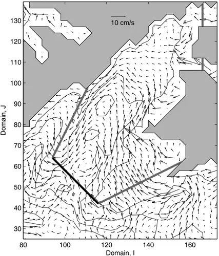
3.3 Circulation in Storfjorden 20

The mean surface circulation is consistent with observations (Skogseth et al., 2005b) and a previous model study (Skogseth et al., 2007). The dominant pattern in the Stor-fjorden basin is a cyclonic surface circulation (Fig. 6), with the main inflow over the eastern half of the sill and across Storfjordbanken, the shallow bank between the sill and Edgeøya. Inflow also occurs through the narrow Freemansundet north of Edgeøya.

25

Surface outflow from the basin is over the western half of the sill and the adjacent ridge stretching northwards toward Spitsbergen.

(10)

OSD

7, 17–49, 2010

F. Geyer et al.

Title Page

Tables Figures

◭ ◮

Back Close

Full Screen / Esc

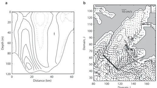
Interactive Discussion across the sill are calculated for strong overflow cases. The average over times with the

strongest overflow identified with bottom cross-sill velocities u_out>20 cm s−1 _(directed

out of the fjord) corresponds to the following flow changes: The outflow leaning on the western slope of the sill is strengthened overall, with an intensification toward the bottom (Fig. 7a). There is a corresponding increase in the inflow strength, both over

5

the middle part of the sill and toward the eastern flank, particularly in the upper 30 m, and through Freemansundet between Edgeøya and Barentsøya. The surface inflow extents further across Storfjordbanken east of the sill (Fig. 7b). The increase in the surface inflow is not balanced by a corresponding increase in the surface outflow over the ridge northwest of the sill.

10

4 Discussion

4.1 Wind forcing of the overflow

Geyer et al. (2009) observed significant coherency between the wind forcing and the dense overflow at the Storfjorden sill for periods longer than 4 days and postulated a wind-driven surface flow into the fjord and a return flow at depth as the

connect-15

ing mechanism. Surface inflow is expected due to Ekman transport in response to wind stress, typically due to winds directed from 45–135◦_{T. We detect the times of}

wind from east-northeast (45–90◦T) and from east-southeast (90–135◦T), and calcu-lated the corresponding ensemble averages. Deviations from the mean circulation are shown in Figs. 8–9. Average surface inflow is enhanced for both east-northeasterlies

20

(Fig. 8) and east-southeasterlies (Fig. 9). The patterns of the two different ensembles, however, vary. The wind from east-southeast transports water infjord across the en-tire southern boundary (Fig. 9), while the wind from east-northeast mainly leads to an increased inflow over the bank east of the sill (Fig. 8). East-northeasterly winds also open the Storfjorden polynya west of Edgeøya (see e.g., Fig. 2 in Smedsrud et al.,

25

(11)

OSD

7, 17–49, 2010

F. Geyer et al.

Title Page

Tables Figures

◭ ◮

Back Close

Full Screen / Esc

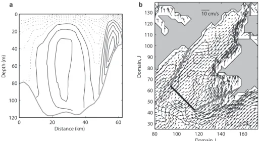
Interactive Discussion The east-northeasterly winds are associated with an increased dense overflow

(Fig. 8a). East-southeasterly winds correspond to enhanced outflow mainly at inter-mediate depths and the weakening of the warm inflow over the eastern part of sill (Fig. 9a). East-northeasterlies push the surface water in Storfjorden westward against the east coast of Spitsbergen. The resulting pileup of water against the coast is the

5

driving force for the southward return flow at depth. This surface response to wind forcing was also observed in a regional model study of the region using fine-scale wind forcing in the absence of ice (Skogseth et al., 2007).

Geyer et al. (2009) suggested that infjord surface Ekman flux had skill to predict overflow strength and variability. The flow distribution over the sill crest for the

east-10

northeasterly winds (Fig. 8a), albeit weaker, closely resembles the distribution for the strongest overflow incidences (Sect. 3; Fig. 7). For the analysis of the model results, the net surface Ekman fluxes in and out of the fjord are calculated from the surface wind stressτ

F_E,x=

τ_y f ρW

;F_E,y=−

τ_x f ρW

(1)

15

integrated across the boundaries of Storfjorden as indicated in Fig. 2. Here

f=1.42×10−4s−1 is the Coriolis parameter andρW=1027 kg m−3is the density of sea

water. The resulting net surface Ekman flux into the fjord is typically strong during the freezing period and is significantly weaker during summer, comparable to the overflow cycle (Fig. 10). During the freezing season large overflow flux is associated with large

20

values ofF_E, however, the opposite is not true. For instance, in early January significant

F_Ehas no discernible overflow flux.

4.2 Polynya events and the overflow

The two main influences on the Storfjorden overflow on time scales longer than the tidal frequencies are the buoyancy forcing from the dense water source at the Storfjorden

25

(12)

measure-OSD

7, 17–49, 2010

F. Geyer et al.

Title Page

Tables Figures

◭ ◮

Back Close

Full Screen / Esc

Interactive Discussion ments in April 2006, during a supercooling event of polynya activity, Skogseth et al.

(2008) trace the high salinity signal and detect it flow past the sill crest 12 to 18 days after the polynya event. This time lag, also consistent with a conservative analytical estimate, compares with the filling time of the basin to the sill level from the start of freezing period. Once the interface has reached the sill level, subsequent events with

5

high salinity pulse are estimated to reach the sill in 1 to 3 days (Skogseth et al., 2008). The ROMS model results do not support a direct polynya-overflow link with a 1–3 days time delay. It is instead dominated by an immediate (one day or less) overflow response to surface winds from east to northeast directions (Fig. 11c).

All seven major polynya events during the freezing season in 2000 can be

con-10

nected to strong easterly wind events (Fig. 11). The polynya opens (gradually increas-ing polynya area,A_P), responding immediately to wind forcing (Fig. 11a). The polynya closes (A_P reduces due to freezing and ice formation) relatively slowly following an opening event. The closing of the polynya occurs a few days to two weeks after the wind forcing ceases. As the ice freezes in the closing polynya, salinity in the polynya

15

region increases (Fig. 11b). Once the polynya has reached freezing temperature, all polynya events lead to ice formation and brine rejection visible as local salinity maxima in the central polynya area (Fig. 11c).

Modeled salinities are too high due to an overestimation of the import of Atlantic Water into the Barents Sea in the intermediate-scale model of the Barents and Kara

20

Seas used in nesting (Budgell, 2005). Relatively saline water entering the polynya region then leads to BSW of high salinity. For comparison, values of maximum salinity observed in the deepest pool of the basin (hence after being diluted from the polynya to the mid-basin) vary between about 34.7 to 35.83 (Skogseth et al., 2005a) with the largest value recorded in April 2002 (Anderson et al., 2004).

25

Salinity maxima typically occurs 5 to 12 days following the maxima inAP. The salinity

(13)

OSD

7, 17–49, 2010

F. Geyer et al.

Title Page

Tables Figures

◭ ◮

Back Close

Full Screen / Esc

Interactive Discussion shown), are dampened out in the center of the basin (station 2, Fig. 11b). The result

is a gradual increase in salinity and density in the basin. Bottom salinity at the sill crest closely follows the salinity at the sill level in the basin but with greater variability (Fig. 11b), possibly due to episodic wind-induced overflow events carrying water from below the sill depth. Some signal propagation from the polynya can of course not be

5

excluded, but the salinity variations at the sill adhere much closer to the wind-driven velocity variations at the sill than to salinity variations upstream. Salinity variations as a cause for the velocity variations at the sill can be excluded as the salinity maxima at the sill are occurring with 1–2 days time lag to the overflow transport maxima.

Lagged-correlation analysis yieldr2=0.78 at 25 days lag between the polynya area

10

and the overflow at the sill. Maximum correlation with the wind stress, on the other hand, is at one day lag (wind leading), 0.55 using wind stress and 0.69 using the favor-able wind stress component from 67.5◦T. All the stated values are significant at 95% confidence. The ocean thus integrates the polynya forcing over several events, consis-tent with Chapman (1999) who found that typical ocean adjustment scale is typically

15

10–20 days depending on the geometry and forcing of the polynya.

The ability of the wind forcing to drive out dense water from behind the sill, visible from strong overflow events not connected to salinity maxima at the sill (Fig. 11) and the dampening of high salinity events in the basin suggest that the dense water production at the polynya acts rather as a background mechanism: The gradual salinity increase

20

in the Storfjorden basin provides the brine-enriched shelf water, which fills up the basin to the sill level and is then flowing over the sill, mainly in the form of wind-driven pulses. Possible excessive mixing in the model could dampen the salinity signal of a polynya event and hinder the detection of propagation from polynya to the sill. The mixing scheme used in this study is state-of-the-art, but Mellor-Yamada schemes typically

25

(14)

OSD

7, 17–49, 2010

F. Geyer et al.

Title Page

Tables Figures

◭ ◮

Back Close

Full Screen / Esc

Interactive Discussion bathymetry in the region (Skogseth et al., 2008).

4.3 Overflow width and height at the sill, and their influence on transport estimates from measurements

The width of the overflow plume is a source of large uncertainty in estimating volume transport from moored observations (Schauer, 1995; Schauer and Fahrbach, 1999;

5

Geyer et al., 2009). Typically a constant width of 15 km is assumed. The model results show that the overflow plume width at the sill crest can vary substantially exceeding 40 km during the overflow maximum in February and early March, thus covering two thirds of the width of the sill and the adjacent slopes (Fig. 12). The episodic wide plume events receive support from the recent observation of BSW over the the easternmost

10

part of the sill (Skogseth et al., 2008). However, if we define the corresponding width,

wcorr, that is required to obtain the overflow volume transport

Q=wcorr

Zz=0

z=−H

uoutd z (2)

from profiles of outflow velocity of BSWu_out at the location corresponding to the sill mooring (station 3), the variability is considerably smaller. Except for a few events

15

when the overflow misses the station, the corresponding overflow width is about 15 km throughout the overflow season (Fig. 12), in agreement with the width assumed in Geyer et al. (2009) and earlier studies (Schauer, 1995; Schauer and Fahrbach, 1999). The extent of the brine-enriched shelf water follows mainly the temperature distribu-tion at the sill (Sect. 3), but cannot be delineated using the velocity distribudistribu-tion. Due

20

to the lack of temperature profiles at the sill, Geyer et al. (2009) estimated the vertical extent of the overflow from velocity profiles. Our model results allow us to assess any systematic errors in the corresponding overflow flux calculations. Figure 13a compares the overflow height at station 3 calculated directly from water-mass characteristics and velocity profiles to that calculated by velocity profiles alone, using the method laid out

25

(15)

OSD

7, 17–49, 2010

F. Geyer et al.

Title Page

Tables Figures

◭ ◮

Back Close

Full Screen / Esc

Interactive Discussion height determined from current profiles agrees reasonably well with the actual height,

so that the method captures the vertical extent of the overflow correctly. For the later and weaker part of the overflow season from May to July, however, the plume thick-ness is substantially overestimated. The overestimation is neither connected to bottom velocities nor temperatures, but rather caused by the outflow of warmer water at

inter-5

mediate layers.

The effects of the plume width and height estimates on the overflow transport are shown in Fig. 13b. The overflow volume transport is calculated in three di_fferent ways. The “actual” overflow volume transport (Q₁) is calculated by integrating the total out-flow of BSW across the sill. Secondly, velocity and hydrographic (T/S) profiles are

ex-10

tracted at station 3 (the mooring location), and the volume transport (Q₂) is calculated using the outflow over the thickness of the BSW identified byT/S properties, assum-ing 15 km width. Finally, the volume transport (Q₃) is calculated using the outflow over the thickness identified by the outflow velocity profiles and assuming 15 km width. The calculation ofQ₃is identical to that from current profile observations from the mooring.

15

Overflow volume transportQ₂is acceptably accurate since the constant width of 15 km is a reasonable approximation and the plume thickness is properly inferred. The over-flow transportQ₃ is correct for a large part of the overflow season, but overestimates the actual transport for the intermittent overflow periods from May to July. Averaged over the 202 days overflow season, overflow volume fluxQ1=0.071±0.076 Sv (±one

20

standard deviation). Current profile based estimate captures both the mean and the variability resulting inQ₃=0.077±0.078 Sv. Q3explains 58% of the variance ofQ1and

on the average agrees to within 10% ofQ1with a standard error of 0.054 Sv.

5 Conclusions

Results from the first realistic simulation of the Storfjorden region are presented. The

25

(16)

OSD

7, 17–49, 2010

F. Geyer et al.

Title Page

Tables Figures

◭ ◮

Back Close

Full Screen / Esc

Interactive Discussion overflow season in Storfjorden. Results are consistent with previously reported

circu-lation patterns and the observations from both the polynya and the overflow region. The overflow volume transport of brine-enriched shelf water (BSW) at the sill is strongly connected to wind forcing. Wind from east-northeast enhances surface inflow across Storfjordbanken between the sill and Edgeøya and a corresponding return flow

5

at depth in the western part of the sill, which strengthens the dense overflow. While the Storfjorden polynya opens in response to easterly winds, causing ice formation and BSW production, the density excess cannot be traced into the basin as a pulse but instead a gradual increase in local salinity and density is seen. The variability of the dense overflow at the sill crest is found to be determined largely by the wind stress. The

10

response of the fjord and hence the overflow to isolated polynya events is at longer time scales (about 25 days), which integrates the buoyancy forcing induced by the polynya over several polynya events. This result suggests that reasonable estimates of ocean response can be obtained from coarse observations of satellite images and surface forcing at steady state or at coarse temporal resolution.

15

The overflow plume width at the sill crest varies, occasionally exceeding 40 km (entire extent of the sill). However, the common constant overflow width assumption used to estimate volume transports from point measurements is shown to hold rather well. Detailed analysis of the model data suggests that, assuming the modeled total overflow transport as benchmark value, the volume flux of the BSW plume can be monitored by

20

a single current profiler at the sill crest capturing 58% of the variability and accurate to within 10% when averaged over the overflow duration.

Acknowledgements. The authors want to thank T. Eldevik for his helpful comments on the manuscript and W. P. Budgell for his support with model runs. This work is funded by the Research Council of Norway, through Bipolar Atlantic Thermohaline Circulation (BIAC) project. 25

(17)

OSD

7, 17–49, 2010

F. Geyer et al.

Title Page

Tables Figures

◭ ◮

Back Close

Full Screen / Esc

References

Aagaard, K., Coachman, L. K., and Carmack, E.: On the halocline of the Arctic Ocean, Deep-Sea Res., 28A, 529–545, 1981. 19

Aagaard, K., Swift, J. H., and Carmack, E.: Thermohaline circulation in the Arctic Mediterranean Seas, J. Geophys. Res., 90, 4833–4846, 1985. 19

5

Anderson, L. G., Falck, E., Jones, E. P., Jutterstr ¨om, S., and Swift, J. H.: Enhanced uptake of atmospheric CO2 during freezing of seawater: a field study in Storfjorden, Svalbard, J.

Geophys. Res., 109, C06004, doi:10.1029/2003JC002120, 2004. 28

Arrigo, K. R., van Dijken, G., and Pabi, S.: Impact of a shrinking Arctic ice cover on marine primary production, Geophys. Res. Lett., 35, L19603, doi:10.1029/2008GL035028, 2008. 10

Bauch, D. P., Schlosser, P., and Fairbanks, R.: Freshwater balance and the sources of deep water and bottom waters in the Arctic Ocean inferred from the distribution of H2

18

O, Prog. Oceanogr., 35, 53–80, 1995. 19

Budgell, W. P.: Numerical simulation of ice-ocean variability in the Barents Sea region towards dynamic downscaling, Ocean Dynam., 55, 370–387, 2005. 21, 28

15

Carmack, E. and Chapman, D. C.: Wind-driven shelf/basin exchange on an Arctic shelf: the joint roles of ice cover extent and shelf-break bathymetry, Geophys. Res. Lett., 30, 1778, doi:10.1029/2003GL017526, 2003.

Chapman, D. C.: Dense water formation beneath a time-dependant coastal polynya, J. Phys. Oceanogr., 29, 807–820, 1999. 29

20

Engedahl, H.: Use of the flow relaxation scheme in a three-dimensional baroclinic model with realistic topography, Tellus, 47A, 365–382, 2009. 21

Ersdal, E. A.: On the tidal forcing of the Storfjorden polynya, M.Sc., Univ. of Bergen, 2009. 23 Fer, I., Skogseth, R., Haugan, P. M., and Jaccard, P.: Observations of the Storfjorden outflow,

Deep-Sea Res. I, 50, 1283–1303, 2003. 19 25

Fer, I., Skogseth, R., and Haugan, P. M.: Mixing of the Storfjorden overflow (Sval-bard Archipelago) inferred from density overturns, J. Geophys. Res., 109, C01005, doi:10.1029/2003JC001968, 2004. 19

Fer, I. and ˚Adlandsvik, B.: Descent and mixing of the overflow plume from Storfjord in Sval-bard: an idealized numerical model study, Ocean Sci., 4, 115-132, 2008, http://www.ocean-30

(18)

OSD

7, 17–49, 2010

F. Geyer et al.

Title Page

Tables Figures

◭ ◮

Back Close

Full Screen / Esc

Geyer, F., Fer, I., and Eldevik, T.: Dense overflow from an Arctic fjord: mean seasonal cycle, variability and wind influence, Cont. Shelf Res., 29, 2110–2121, 2009. 20, 24, 25, 26, 27, 30, 48, 49

H ¨akkinen, S. and Mellor, G. L.: Modeling the seasonal variability of a coupled Arctic ice-ocean system, J. Geophys. Res., 97, 20285–20403, 1992. 21

5

Hunke, E. C. and Dukowicz, J. K.: An elastic-viscous-plastic model for sea ice dynamics, J. Phys. Oceanogr., 27, 1849–1867, 1997. 21

Hunke, E. C.: Viscous-plastic sea ice dynamics with the EVP model: linearization issues, J. Comp. Physiol., 170, 18–38, 2001. 21

Ilicak, M., ¨Ozg ¨okmen, T. M., Peters, H., Baumert, H. Z., and Iskandarani, M.: Performance of 10

two-equation turbulence closures in three-dimensional simulations of the Red Sea overflow, Ocean Model., 24, 122–139, 2008. 29

Jungclaus, J. H., Backhaus, J. O., and Fohrmann, H.: Outflow of dense waters from the Stor-fjord at Svalbard: a numerical model study, J. Geophys. Res., 100, 24719–24728, 1995. 20

15

Kalnay, E., Kanamitsu, M., Kistler, R., Collins, W., Deaven, D., Gandin, L., Iredell, M., Saha, S., White, G., Woollen, J., Zhu, Y., Chelliah, M., Ebisuzaki, W., Higgins, W., Janowiak, J., Mo, K. C., Ropelewski, C., Wang, J., Leetmaa, A., Reynolds, R., Jenne, R., and Joseph, D.: The NCEP/NCAR 40-year reanalysis project, B. Am. Meteorol. Soc., 77, 437–471, 1996. 22 Loeng, H.: Features of the physical oceanographic conditions in the Barents Sea, Polar Res., 20

10, 5–18, 1991. 24

Mellor, G. L. and Yamada, T.: Development of a turbulent closure model for geophysical fluid problems, Rev. Geophys. Space Ge., 20, 851–875, 1982. 21

Mellor, G. L. and Kantha, L.: An ice-ocean coupled model, J. Geophys. Res., 94, 10937–10954, 1989. 21

25

Perovich, D. K., Richter-Menge, J. A., Jones, K. F., and Light, B.: Sunlight, water, and ice: extreme Arctic sea ice melt during the summer of 2007, Geophys. Res. Lett., 35, L11501, doi:10.1029/2008gl034007, 2008.

Quadfasel, D., Rudels, B., and Kurz, K.: Outflow of dense water from a Svalbard fjord into the Fram Strait, Deep-Sea Res., 35, 1143–1150, 1988. 19

30

(19)

OSD

7, 17–49, 2010

F. Geyer et al.

Title Page

Tables Figures

◭ ◮

Back Close

Full Screen / Esc

Schauer, U.: The release of brine-enriched shelf water from the Storfjord into the Norwegian Sea, J. Geophys. Res., 100, 16015–16028, 1995. 19, 30

Schauer, U. and Fahrbach, E.: A dense bottom water plume in the western Barents Sea: down-stream modification and interannual variability, Deep-Sea Res., Pt. I, 46, 2095–2108, 1999. 30

5

Shchepetkin, A. F. and McWilliams, J. C.: The regional oceanic modeling system (ROMS): a split-explicit, free-surface, topography-following-coordinate oceanic model, Ocean Model., 9, 347–404, 2005. 21

Skogseth, R., Fer, I., and Haugan, P. M.: Dense-water production and overflow from an Arctic coastal polynya in Storfjorden, in: The Nordic Seas: An Integrated Perspective, Geophysical 10

Monograph Series, vol. 158, edited by: Drange, H., Dokken, T., Furevik, T., Gerdes, R., and Berger, W., AGU, Washington, DC, 73–88, 2005a. 19, 22, 23, 28

Skogseth, R., Haugan, P. M., and Jakobsson, M.: Watermass transformations in Storfjorden, Cont. Shelf Res., 25, 667–695, 2005b. 19, 25

Skogseth, R., Sandvik, A. D., and Asplin, L.: Wind and tidal forcing on the meso-scale cirulation 15

in Storfjorden, Svalbard, Cont. Shelf Res., 27, 208–227, 2007. 19, 22, 25, 27

Skogseth, R., Smedsrud, L. H., Nilsen, F., and Fer, I.: Observations of hydrography and down-flow of brine-enriched shelf water in the Storfjorden polynya, Svalbard, J. Geophys. Res., 113, C08049, doi:10.1029/2007JC004452, 2008. 19, 20, 28, 30

Skogseth, R., Nilsen, F., and Smedsrud, L. H.: Supercooled water in an Arctic polynya: obser-20

vations and modeling, J. Glaciol., 55(189), 43–52, 2009. 22

Smedsrud, L. H., Budgell, W. P., Jenkins, A. D., and ˚Adlandsvik, B.: Fine-scale sea-ice mod-elling of the Storfjorden polynya, Ann. Glaciol., 44, 73–79, 2006. 20, 21, 22, 23, 26

Song, T. and Haidvogel, D.: A semi-explicit ocean circulation model using a generalized topography-following coordinate system, J. Comp. Physiol., 115, 228–244, 1994. 21

25

Warner, J. C. and Geyer, W. R.: Numerical modelling of an estuary: a comprehensive skill assessment, J. Geophys. Res. 110, C05001, doi:10.1029/2004JC002691, 2005. 21

Warner, J. C., Sherwood, C. R., Arango, H. G., and Signell, R. P.: Performance of four turbu-lence closure models implemented using a generic length scale method, Ocean Model. 8, 81–113, 2005. 21

30

(20)

OSD

7, 17–49, 2010

F. Geyer et al.

Title Page

Tables Figures

◭ ◮

Back Close

Full Screen / Esc

Winsor, P. and Bj ¨ork, G.: Polynya activity in the Arctic Ocean from 1958–1997, J. Geophys. Res., 105, 8789–8803, 2000. 19

(21)

OSD

7, 17–49, 2010

F. Geyer et al.

Title Page

Tables Figures

◭ ◮

Back Close

Full Screen / Esc

Interactive Discussion 0o

6o_E

12oE 18oE 24 o_E

75o

N 76o

N 77o

N 78o

N 79o

N 80o

N 81o

N

Spitsbergen

Storfjordrenna Storfjorden

−3500

−3000

−2500

−2000

−1500

−1000

−500 0

Fig. 1.Map of Storfjorden and the Svalbard archipelago. The ROMS model domain covers the

(22)

OSD

7, 17–49, 2010

F. Geyer et al.

Title Page

Tables Figures

◭ ◮

Back Close

Full Screen / Esc

3

2

1 Spitsbergen

Edgeøya

Domain, I

Domain, J

polynya

Storfjordbanken

Barents

−

øya

80 100 120 140 160

30 40 50 60 70 80 90 100 110 120 130 140

Fig. 2. Storfjorden with stations 1–3 (squares), thick lines delimit the extent of the Storfjorden

(23)

OSD

7, 17–49, 2010

F. Geyer et al.

Title Page

Tables Figures

◭ ◮

Back Close

Full Screen / Esc

Interactive Discussion −2

−1 0 1 2

T (

°

C)

a) T

cm s−1

−20 −15 −10 −5 0 5 10 15 20

Oct99 Jan00 Apr00

−100 −80 −60 −40 −20

mab

b) X−sill

Time (mmmyy)

Fig. 3. Time series of (a) bottom temperature and (b) cross-sill component of the velocity

(24)

OSD

7, 17–49, 2010

F. Geyer et al.

Title Page

Tables Figures

◭ ◮

Back Close

Full Screen / Esc

−120 −100 −80 −60 −40 −20 0

Depth

Inflow Outflow

−300 −25 −20 −15 −10 −5 0 5 10 15 20 25

5 10 15 20 25 30

v (cm s−1)

Occurrence (%)

−3 −2 −1 0 1 2 3 T

T (

°

C)

a

b

Fig. 4. (a)Average current for the cross-sill component of the velocity grouped according to the

bottom current in 5 cm s−1

(25)

OSD

7, 17–49, 2010

F. Geyer et al.

Title Page

Tables Figures

◭ ◮

Back Close

Full Screen / Esc

−1.75

−1.25

−0.75

−0.25 0.25 0.75 1.25

Distance (km)

Depth (m)

BSW

MAW

0 10 20 30 40 50 60

0

20

40

60

80

100

120

T (oC)

Fig. 5. Along-sill section of mean temperature (color-coded) and cross-sill velocity (white

con-tours) for the overflow season. Contour lines are drawn in 2.5 cm s−1

(26)

OSD

7, 17–49, 2010

F. Geyer et al.

Title Page

Tables Figures

◭ ◮

Back Close

Full Screen / Esc

10 cm/s

Domain, I

Domain, J

80 100 120 140 160

30 40 50 60 70 80 90 100 110 120 130

Fig. 6. Mean surface circulation in Storfjorden. Isobaths are drawn at 50 m intervals. Thick

(27)

OSD

7, 17–49, 2010

F. Geyer et al.

Title Page

Tables Figures

◭ ◮

Back Close

Full Screen / Esc

Distance (km)

Depth (m)

0 20 40 60

0

20

40

60

80

100

120

10 cm/s

Domain, I

Domain, J

80 100 120 140 160

30 40 50 60 70 80 90 100 110 120 130

a b

Fig. 7. (a)Difference from mean cross-sill velocity for cases of strong outflow (cross-sill velocity

(28)

OSD

7, 17–49, 2010

F. Geyer et al.

Title Page

Tables Figures

◭ ◮

Back Close

Full Screen / Esc

10 cm/s

Domain, I

Domain, J

80 100 120 140 160 30

40 50 60 70 80 90 100 110 120 130

Distance (km)

Depth (m)

0 20 40 60 0

20

40

60

80

100

120

a b

Fig. 8. (a)Difference from mean cross-sill velocity for times of east-northeasterly winds (45–

90◦_{T, 86 of 365 days). Contour lines are drawn in 1 cm s}−1

(29)

OSD

7, 17–49, 2010

F. Geyer et al.

Title Page

Tables Figures

◭ ◮

Back Close

Full Screen / Esc

10 cm/s

Domain, I

Domain, J

80 100 120 140 160 30

40 50 60 70 80 90 100 110 120 130

Distance (km)

Depth (m)

0 20 40 60

0

20

40

60

80

100

120

a b

Fig. 9. (a)Difference from mean cross-sill velocity for times of east-southeasterly winds (90–

135◦_{T, 64 of 365 days). Contour lines are drawn in 1 cm s}−1

(30)

OSD

7, 17–49, 2010

F. Geyer et al.

Title Page

Tables Figures

◭ ◮

Back Close

Full Screen / Esc

Jan Apr Jul Oct Jan Apr Jul Oct Jan

0 0.05 0.1 0.15 0.2 0.25

0.07

Time (month)

Q (Sv)

Fig. 10.Time series of weekly net surface Ekman fluxF_Einto the fjord (black line) in 1999–2000

(31)

OSD

7, 17–49, 2010

F. Geyer et al.

Title Page

Tables Figures

◭ ◮

Back Close

Full Screen / Esc

0 2 4 6

1000

×

A

P

(km

2 )

A P

34.5 35 35.5 36

P

2

3

S

Jan Feb Mar Apr

0 0.25 0.5

Q

Q (Sv)

0 0.5 1

τ w

(Pa)

−0.5 0 0.5 1

τ ENE

(Pa)

a

c b

Fig. 11.Comparison of daily time series for(a)polynya areaA_P(gray shading) and wind stress

(32)

OSD

7, 17–49, 2010

F. Geyer et al.

Title Page

Tables Figures

◭ ◮

Back Close

Full Screen / Esc

Jan Feb Mar Apr May Jun Jul

0 10 20 30 40 50 60

Time [month]

Width [km]

Fig. 12.Time series of overflow widthw (grey) and corresponding overflow widthw_corr(black)

(33)

OSD

7, 17–49, 2010

F. Geyer et al.

Title Page

Tables Figures

◭ ◮

Back Close

Full Screen / Esc

0 50 100 150

Overflow Height (m)

Jan Feb Mar Apr May Jun Jul

0 0.1 0.2 0.3 0.4 0.5

Volume Flux (Sv)

a

b

Fig. 13. (a)Comparison of overflow height calculated from velocity profiles following the method