FUNDAÇÃO GETÚLIO VARGAS
ESCOLA DE ECONOMIA DE EMPRESAS DE SÃO PAULO
LUCA CAMILLA WERTH
TITLE:
BRAZIL’S 2014 PRESIDENTIAL ELECTIONS: THE INTERCONNECTION BETWEEN ELECTION NEWS AND STOCK MARKET BEHAVIOUR
SÃO PAULO
FUNDAÇÃO GETÚLIO VARGAS
ESCOLA DE ECONOMIA DE EMPRESAS DE SÃO PAULO
LUCA CAMILLA WERTH
TITLE:
BRAZIL’S 2014 PRESIDENTIAL ELECTIONS: THE INTERCONNECTION BETWEEN ELECTION NEWS AND STOCK MARKET BEHAVIOUR
SÃO PAULO
2016
Dissertação apresentada à Escola de Economia de Empresas de São Paulo da Fundação Getúlio Vargas, como requisito para obtenção do título de Mestre Profissional em Economia.
Campo do Conhecimento: International Master in Finance
Werth, Luca Camilla.
Brazil’s 2014 Presidential Elections: The Interconnection between Election News and Stock Market Behaviour / João Mergulhão. - 2016.
50 f.
Orientador: João Mergulhão
Dissertação (MPFE) - Escola de Economia de São Paulo.
1. Mercado financeiro. 2. Ações (Finanças). 3. Eleições – Brasil. I.
Mergulhão, João. II. Dissertação (MPFE) - Escola de Economia de São Paulo. III. Título.
LUCA CAMILLA WERTH
TITLE:
BRAZIL’S 2014 PRESIDENTIAL ELECTIONS: THE INTERCONNECTION BETWEEN ELECTION NEWS AND STOCK MARKET BEHAVIOUR
Dissertação apresentada à Escola de Economia de Empresas de São Paulo da Fundação Getúlio Vargas, como requisito para obtenção do título de Mestre Profissional em Economia.
Campo do Conhecimento: International Master in Finance
Data de Aprovação: ___/___/____.
Banca Examinadora:
_________________________________ Prof Dr João Mergulhão (advisor)
_________________________________ Assoc Prof Dr André Castro Silva (advisor)
RESUMO
Este estudo investiga se houve comportamento anormal no mercado de ações no Brasil
decorrente de notícias sobre as últimas eleições presidenciais brasileiras (através da
utilização de sondagens), realizadas em outubro de 2014. Utilizando uma metodologia
de estudos de evento (event studies), a investigação sobre o Ibovespa e a Petrobras
sugere que, nos períodos em que Dilma melhorava a sua posição nas sondagens
existiram retornos anormais negativos e, nos períodos em que Rousseff piorava a sua
posição, existiram retornos anormais positivos. Além disso, a volatilidade foi bastante
elevada durante o período eleitoral tendo o volume de transações aumentado
ligeiramente.
ABSTRACT
This study researches whether there has been abnormal stock market behaviour in Brazil as a consequence of election news (observed via opinion polls), regarding the last Brazilian presidential election, held in October 2014. Via applying event study methodology, the research on the Ibovespa and Petrobras suggests that events in which Rousseff was gaining in share have been subject to negative abnormal returns, and events where Rousseff was loosing in share have led to positive abnormal returns. Moreover, volatility has been significantly elevated during the election period and volume has been found to have slightly increased.
TABLE OF CONTENTS
1 Introduction p. 9
2 Analytical Framework p. 11
2.1 Theoretical Notions and Literature Review p. 11
2.2 Analytical Framework: Event Studies p. 15
2.3 Application and Data Selection p. 18
2.3.1 Expected Values and Modelling p. 18 2.3.2 Application of Event Studies p. 21
3 Analysis p. 24
3.1 Market Returns p. 25
3.2 Volatility p. 27
3.3 Volume p. 32
3.4 Government Related Stocks p. 35
3.4.1 Petrobras p. 35
3.4.2 Vale p. 35
4 Robustness, Further Research and Concluding Remarks p. 36
Appendices
Appendix 1 – Additional Data on the EEM p. 44
Appendix 2 – Additional Data on Poll Releases p. 45
Appendix 3 – Descriptive Statistics on the Data Sets p. 46
Appendix 4 – Volatility Event Study p. 47
Appendix 5 – Plots of Ibovespa’s post election CAR p. 47
Appendix 6 – Event study: Petrobras p. 48
Appendix 7 – Event study: Vale p. 49
Appendix 8 – Event study: Merval p. 50
1 Introduction
“The Brazilian unit of Banco Santander has fired an analyst and other employees involved in the publication of a client note critical of President Dilma Rousseff's economic policies” (Jelmayer & Magalhaes, 2014).
This statement clearly highlights that there is a controversial point of intersection between the so-called political world and the financial sector. Within a newspaper article of the Wall Street Journal, Jelmayer and Magalhaes (2014) state that the report in question, responsible for the expulsion of several employees, was concerned with a warning of wealthy clients to prepare for the outcome of the (back then) ‘upcoming’ Brazilian elections. It was stated that when the incumbent president Rousseff was re-elected the overall stock market might suffer. This notion is based on the fact that “Brazil's stock market has rallied repeatedly in recent weeks upon the release of a respected public-opinion poll showing Ms. Rousseff's lead slipping” (Jelmayer & Magalhaes, 2014, p.1). The incident received public and political attention, cumulating in former President Lula da Silva’s rather harsh statement: “This girl doesn’t understand squat about Brazil […] they should fire her and give me her Bonus. There’s no place in the world where Santander earns more money than in Brazil” (Margolis, 2014, p.1)1. Santander apologised publicly to Rousseff and laid of the analysts in question; roughly one year later, one of the fired analysts, Sinara Polycarpo, judicially obtained 450 R$2 as an indemnity for moral damages (Globo G1, 2015). These events clearly highlight that the interplay between political and financial systems is contentious, and to gain an
1
The statement above is a translation of Lula’s words, which published within a Bloomberg View article. The Brazilian news network Globo c
ited Lula’s comment as follows: “manter uma mulher dessa num cargo de chefia, sinceramente …Pode mandar embora. E dá o bônus dela pra mim” (G1 Globo, 2014: 1). However, the Brazilian financial news website InfoMoney differently quoted Lula’s statement: “essa moça não entende p***a nenhuma de Brasil e de governo Dilma” (Salomão, 2014: 1).
2
academic perspective on the politically charged and opinionated issue, this paper aims for researching whether pre-election trends are impacting overall stock market behaviour. In this sense, the paper is concerned with answering the subsequent research question:
Have election trends, as observed via opinion polls, been impacting Brazilian market
behaviour, in regard to IBovespa’s returns, volatility and volume, and the returns of
governmentally related stocks?
Within the following, it is investigated whether there is an impact existent, the null hypotheses of no impact (zero abnormal returns, abnormal volume and abnormal volatility) are tested. Furthermore, the two governmentally related stocks of Petrobras and Vale are tested for abnormal returns in relation to election news.
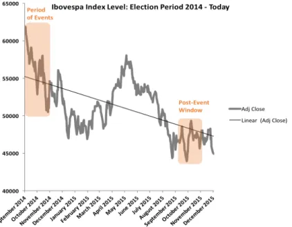
In hindsight, it is observable that since the final presidential election (October 26, 2014) the Ibovespa has been following a downward trend. See Figure 1 below3:
Figure 1: Index Level Ibovespa – September 2014 until December 2015
3
In order to additionally validate the significance, the study introduces a robustness test of running the very same methodology that has been used for testing contingent abnormal returns within the Brazilian pre-election period on the Argentinian stock index MERVAL.
The following section is concerned with providing relevant background information regarding the theoretical frameworks of the subject; further it resumes pertinent background information and outlines the analytical framework and methodology of the study. Second, the analysis section deals with researching the actual impacts of market returns, volatility, volume, and governmentally related stocks in regard to election trends in Brazil. Finally, a concluding part is concerned with making sense of the findings and placing them in the wider context of political environment as well as running the ‘placebo’ study of Argentina’s stock index.
2 Analytical Framework
2.1 Theoretical Notions and Literature Review
There are several theoretical notions and concepts to be found within academic literature, drawing upon different kinds of interplays between politics and financial concerns:
highest possible productivity, otherwise a merger/ acquisition was not necessary or possible. Based on this idea, upcoming elections in a democratic setting bring along the spirit of change, that is hopefully for the better as well, or at least for matching the people’s ideas with governmental composition.
In this regard, the results of Allvine and O’Neill (1980) show that there is a positive correlation between presidential election cycles and stock market behaviour. Their study is concerned with the United State’s election cycle; they found an upward trend over a two-year period prior to presidential elections. This was confirmed by studies of Johnson et al. (1999), who found that within the second part of the presidency stock returns were significantly higher, implying that stock market trends are somehow following election cycles. Panzalis et al. (2000) confirmed these results on an international level. They also found positive abnormal returns when election week has been approaching.
There are several differing theories that are dealing with explaining the relationship of a country’s stock market behaviour and its correlation to political news in general, as well as to elections: In that sense, the model of the political business cycle was developed by Nordhaus in 1975; which is explaining the manipulating influence of political parties in order to attempt wining re-elections. Further, Hibbs (1977) proposed the so-called partisan theory which draws on the differing stresses of labour versus business oriented parties.
the Efficient Market Hypothesis (EMH), may simplified be described as a market environment in which (stock-) prices fully reflect all available information. Fama (1965) was the first to mention the concept and in 1970, Fama classified three distinct forms of market efficiency, a weak, a semi-strong, and a strong form of market efficiency, dependent on the market’s level of information accessibility and spread. In that sense, the possibility of abnormal returns may be misleadingly interpreted as a violation of the efficient market hypothesis: However, since election periods are greatly defined by uncertainty, which is reflected in possibly huge price movements. ‘Abnormal’ returns that might be observed after the release of election related news, such as opinion polls, are rather a confirmation of the EMH’s concept of prices (and price-movements) reflecting the overall market sentiment, as fostered by the available information. The velocity of the market’s intake of the news then defines the level of market efficiency4.
Also related to the subject of political and financial interaction, Goldman, Rocholl and So (2009), show political connection, as in companies with politically linked boards have a compelling impact on the value of these companies5.
Medeiros & Roriz (2014) have been looking into the equity risk premium by means of the 2004 US Presidential Election: They found that stocks which are highly exposed to the market tend to suffer in periods of political uncertainty and that equity prices possibly reflect uncertainty linked to elections.
Moreover, Bialkowski, Gottschalk and Wisniewski (2008) have been looking at stock market volatility during periods of elections, studying 27 countries: They found
4
Additionally, it should be mentioned that defining the actual level of Market Efficiency in the real world is not an easy task, since markets are opaque entities. Nevertheless, there is overall agreement that emerging markets such as the Brazilian market are rather defined by a week or semi-strong form of efficiency.
5
that stock market volatility is indeed substantially increased during periods of national elections. Using a volatility event study within the framework of a GARCH (1,1) volatility model, they examined 134 elections, and found that “a strong abnormal rise starts on Election Day” (Bialkowski et al, 2008, p.1947), whereas the market starts to settle down “after around 15 trading days following the event” (ibid). Additionally, the research drew on the determinants of excess volatility, the authors found, the margin of victory, as in the closeness of the opponents, to be a significant determining factor. Further, “a change in political orientation of the executive also adds to volatility of stock prices” (ibid)6. Drawing upon the compensation of investors taking political risk while holding stock during election periods, they did not find positive abnormal returns: “down and upwards moves occur with almost equal probability” (Bialkowski et al, 2008: 1949).
Bringing the gathered information together leads to somewhat confusing results: on a macro level, financial election cycles with market uplifts around election periods occur (Allvine and O’Neill (1980); Johnson et al. (1999); Panzalis et al. (2000)); however, on a micro level, when looking specifically into small event windows around election day Bialkowski, Gottschalk and Wisniewski (2008) did not find potential for positive abnormal returns on an international level.
Building upon the knowledge studies such as Bialkowski, Gottschalk and Wisniewski’s provided, this study researches the possible impact of the 2014 Brazilian Presidential Elections on overall market behaviour, in depth. Due to the vigorous empirical nature of the research, the data has been analysed by utilising the widely used concept of abnormal returns in an event study context. The following section is
6
concerned with providing theoretical insights into the event study methodology as an underlying concept.
2.2 Analytical Framework: Event Studies
Event studies have been widely used within financial research to investigate investors’ responses to specific events. Mostly, Event study methodology is used to examine the impact of firm specific events such as the issuance of new debt or the announcements of earnings. However, it has also been utilised to investigate the impact of events concerning overall economic condition7. During periods of events, new information is processed by the markets which conceivably leads to abnormal returns, (see Liu, 2007).
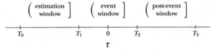
MacKinlay (1997) suggests key steps to follow to successfully conduct an event study: First, the Event has to be defined:
Figure 2: Timeline of an Event Study (see MacKinlay, 1997, p. 20)
Here, the estimation window is the basis of the calculation of a series’ expected values. The event window is the actual period of concern where the possibly abnormal returns may have occurred. The post-event window is considered when it is of interested what happened to the prices after the actual event8.
7
For instance, change in legislation or the impact of elections. 8
Next, the expected or normal values (i.e. returns) of a series are calculated based on data from the estimation window. Here, differing approaches are available, dependent on which type of series is under observation. The most common approach to estimate a series of expected returns is based on the Market Model: Which is an ordinary least square approach of regressing a series of expected returns, by means of an intercept estimation (�!); a market-based beta estimate (�!), which describes the firm’s relationship to overall market-movements; the actual returns of the market (�!,!); as
well as an error term (�!,!)9.
�(�!,!) = �! +�!�!,!+�!,!, �!,! ~ �(0,�!,!!)
After defining the expected returns for a specific period, the abnormal returns have to be calculated: Following logical reasoning, abnormal returns within a certain period can be defined as the difference between actual (observed) returns minus the expected returns (Serra, 2002)10.
��!,! =�!,!−�(�!,!)
Further, the measure of cumulative abnormal returns (CAR) provides the cumulative sum of observed abnormal returns over the event period. The fact that during the period under consideration in this study, right before the election, polls have been released on an almost daily basis, which makes it difficult to calculate CARs. Most of the event periods in use have a length of only one day, to avoid interference of differing events
9
This can be classified as a regression based approach, according to Cable and Holland’s study in 1999. 10
with one-another11. The average abnormal return (AvAR) provides the mean amount of all the abnormal returns within the event period12.
The next step is defining whether the observed abnormal returns as well as their cumulative sum are sufficiently abnormal to be statistically significant. This can be observed via hypothesis testing of the abnormal returns: The null hypothesis of no abnormal returns (AR=0) can be tested against various alternatives of either negative abnormal returns (AR<0), positive abnormal returns (AR>0), or abnormal returns that are different from zero (AR≠0), depending on expectations about the possible impact of the event. Then, a test statistic is computed which has to be compared to a critical value13. The test statistic is computed as follows, whereas SE is the standard error retrieved from the regression14. (see Brooks 2008, Liu, 2007; Bialkowski, Gottschalk & Wisniewski, 2008).
�!
,!
!"= ��!,!
��!
�!"# =
���!"!#$
!"#$%!(! !,!!) �
!−�!+1∗��!
Since this study attempts to not only investigate abnormal returns but also abnormal volatility and abnormal volume, further modelling assumptions have to be clarified.
11
However, the study computes a five-day CAR after the final Election, when no further interference due to other poll releases can be happening.
12
Within this study, the AvAR is the average of all day-one abnormal returns among the different events of poll releases or actual election rounds, this will be further described in the following section.
13
For reasons of simplicity, normality is assumed, (see Appendix 3 for the kurtosis, and skewness results of the data set).
14
Since the null hypothesis can be defined as AR of zero, the numerator of the AR minus its expectation under the null hypothesis (zero) can be simply stated as AR: In stead of: �!"= !"!!!
!"#(!"!) , (the same
In regard to modelling volatility, this paper takes a GARCH(1,1) approach:
�(�!,!)= �! +�!�!,!+�𝑖,!, �!,! ~ �(0,�!,!!)
�!!,!= �+�
!�!!,!!!+�!�!!,!!!
�!,! can be described as the conditional volatility, at time t. The GARCH(1,1) process is
a weighted function of a long term average value (dependent on �), volatility information on the previous day (�!�
!,!!!!) and the model’s fitted variance from the previous day (�!�
!,!!!!), (see Brooks, 2008, Chapter 8). The unconditional volatility is describing the normal volatility and will be discussed in the next section.
Moreover, the study models volume by using a mere mean approach, in that sense, the estimation period’s mean volume is defined as the expected value of volume.
2.3 Application and Data Selection
2.3.1 Expected Values and Modelling
The data is retrieved from www.finance.yahoo.com15. Within this study, the estimation window, which is used to model the expected values of normal returns, has the length of 600 observations, starting on October 10, 2011. Since the Ibovespa is an index itself, the market model has to be applied using another broader market index that has a relation to the index in question: Within this study, two models have been used: First, the S&P500 was used as a market proxy for modelling the Ibovespa’s expected returns as well as for Vale’s and Petrobras’ expected returns, since this is a less biased proxy than the Ibovespa index itself16. As a second model the study uses the exchange traded fund EEM (iShares MSCI Emerging Markets ETF)17 as a market proxy to model expected returns – see Appendix 1 for information on the ETF’s composition.
Using OLS regression, expected returns of IBovespa based on the 600 Observations, starting on October 10, 2011, can be described as follows:
�����!&
!: �[�^!"#$]= −0.001+0.92�!&! ���.�!:35.2%
�����
!!": �[�^!"#$]= −0.0002+0.70�!!" ���.�!:50.3%
Regarding volatility, within the framework of this paper, the conditional volatility �!,! has been used as the ‘actual’ volatility value at time t, whereas the normal/ expected volatility value is defined by the unconditional volatility �. Here, � is defined by the squared variance of !, !"#$%&#$'( !"#$%& using 599 residuals stemming from the
regressions.
15
Index data on the IBovespa: ^bvsp; on the S&P500:^gspc; on Vale: vale; on Petrobras: petr3.sa and
petr4.sa; on iShares MSCI Emerging Markets ETF: EEM
16
The Ibovespa is subject of a great deal of affection by movements of the two stocks, because they make up a large part of the index’s composition.
17
�����!&
!: �^!"#$ =1.10%
�����
!!": �^!"#$ =0.96%
Furthermore, the GARCH(1,1) parameters for conditional volatility have been estimated using a Maximum Likelihood approach18:
�����!&!: �
^!!"#$,!= 0.00001+0.03�^!!"#$,!!!+0.89�^!!"#$,!!!
�����
!!": �^!!"#$,!= 0.00002+0.09�^!!"#$,!!!+0.73�^!!"#$,!!!
In regards to modelling expected volume, academia does not provide a clear-cut way to obtain very accurate results. Hence, this research simply models expected volume by taking the mean of Ibovespa’s trading volume over the estimation period. First, a 600 observations model has been used, starting at October 10, 2011 and ending at April 11, 2014. In mid 2013, Brazil lived through a period of riots and public unrest, which supposedly especially impacted the trading volume, leading to a phase of highly volatile volumes. Since this may bias the expected mean value of the index’s volume, additionally a 400-observation average model has been applied.
����� ø!"#,
!"" !"#$%&'()*+#: �[���!] =3,796,067
����� ø!"#,
!"" !"#$%&'()*+#: �[���!] =3,416,666
Following a similar approach than the one of modelling Ibovespa’s expected returns, Vale’s returns can be described as follows:
�����!&
!: �[�!"#$]= −0.002+1.49�!&! ���.�!:36.3%
�����!!": �[�!"#$]= −0.0009+1.16�!!" ���.�!:55.0%
18
��� =−!
!ln 2� − !
!ln �^!"#$,! − !
! !
^!"#$,! !
!
When considering the returns of Petrobras, the study compares two different types of stocks available on Petrobras, the ‘usual’ (Petr3) stock, which comes with all the features of regular common stock, as well as the preferred stock (Petr4), which comes along with the features of preferred stock, that can very simply be described as privileged remuneration, on the costs of no voting rights. Both stocks can respectively be described as follows:
�����!&!: �(�!"#$!)= −0.002+1.13�!&
! ���.�!:18.2%
�����
!!": �(�!"#$!)= −0.001+0.86�!!" ���.�!:26.7%
�����!&
!: �(�!"#$!)= −0.0007+1.02�!&! ���.�!:16.0%
�����
!!": �(�!"#$!)= −0.0001+0.86�!!" ���.�!:28.4%
The next section is concerned with describing the approach towards the actual testing of abnormality during the election period via applying event study methodology and graphical data analysis.
2.3.2 Application of Event Studies
On the basis of the above-mentioned expected values, several event studies were conducted, to test whether there was indeed abnormal stock market behaviour related to news about the upcoming election. In this regard, eight events have been selected to be tested; two of these eight events are the actual election results (round one, October 5, 2014; and round two, October 26, 2014)19. Further, the eight events stem from a period
19
which is referred to in this study as ‘period of events’, starting on October 03, 2014 and ending on October 31, 2014. Hence, all eight events are part of this ‘period of events’ of 21 observations.
Since opinion polls were published quite frequently, and by several institutions, a system of event selection has been employed that attempts to ensure that the single events are not overly biasing one-another20. Further, the events were categorised into two groups dependent on whether the then-incumbent (and now re-elected) President Dilma Rousseff (PT)21 was relatively gaining or loosing in share. In that sense, the type I events are defined as events when Rousseff was relatively gaining in share. Type II Events, are defined as events when Dilma was relatively loosing in share. Both event types have four observations each, whereas type II events, can be described as events when challenger Aécio Neves (PSDB)22 was relatively gaining in share, apart from the first event, which was still prior the first round of election and more challengers were still in the race. However, only the first two candidates (Rousseff and Neves) were allowed to enter the second round.
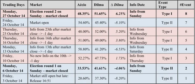
Table 1 below summarises the events that have been selected for the event study tests, whereas Type I events can be observed in red, and Type II Events in blue. The bolded dates refer to the actual first and second election round. New results have been published very frequently, and since it was a close race, the lead has been reversed quite often; therefore, the window length has been set to one day, except for the last event,
20
However in reality, it is extremely challenging to concretely measure the impact of the different poll events upon each other.
21
The PT (Partido dos Trabalhadores), ‘Workers’ Party’ is the Brazilian Labour party, which stresses labour and social political issues.
22
where the event window has a length of two to five trading days23; here, CARs can properly calculated.
The percentage values of the candidates are based on data from
www.eleicoes2014.com.br/pesquisa-eleitoral-para-presidente, as well as other news websites, whereas the mean was taken when more than one poll was published on a given day. Appendix 2 provides a detailed list on which date, at which time and by whom the polls were released, clarifying how the poll release date has been made fit to trading days. When a poll was released during the Bovespa’s opening hours, it enters into market information on the same day, when the release was after market close, the study considers the information to be valid for the next day.
Finally, the abnormal values for each event have been computed and their significance has been tested. For the last event abnormal values have been computed for day one to day five, and on their cumulative sums (CAR/ CAVlm)24.
Table 1: Poll Events (based on Eleições 2014 (2014, a&b); see Appendix 2 for a detailed list of poll releases)
23
Since the last event is already after the final election, there cannot be any interference. 24
Whereas ‘CAR/ CAVlm’ stands for cumulative abnormal returns, and –volume.
Trading Days Market Aécio Dilma ∆ Dilma Info Date Event
Type #Event
Monday, 27 October 14
Election round 2 on
Sunday – market closed 48.35% 51.65% 6.25%
Info from
Sunday Type I 8
Friday,
24 October 14 Market open 54.60% 45.40% -8.10% Type II 7 Thursday,
23 October 14
Info from 23th after market
close –> -1 day 48.00% 52.00% 5.20%
Info from
Wednesday Type I 6 Thursday,
16 October 14
Info from 16th after market
close –> -1 day 51.00% 49.00% 3.80%
Info from
Wednesday Type I 5 Monday,
13 October 14
Info from 13th after market
close –> -1 day 58.80% 41.20% -6.53%
Info from
Saturday Type II 4 Friday,
10 October 14
No new Info on the 10th –>
-1 day 52.27% 47.73% 1.73%
Info from
Thursday Type I 3 Monday,
6 October 14
Election round 1 on
Sunday – market closed 33.53% 41.61% -4.06%
Info from
Sunday Type II 2
Friday, 3 October 14
Market still open but late:
3 Analysis
During the election period, graphs plotting the results of opinion polls, such as the ones below, were everywhere. Politicians, newspapers, as well as to a certain deal academia and many other actors were battling via headlines over headlines. The Brazilian election was receiving a great deal of media attention, not just in Brazil itself but also in the rest of the world. One could argue that the huge level of international media attention was mainly due to the fact that the election results might have an effect on Brazil’s market conditions, which is arguably of great interest to many international investors, who view it as a promising emerging market; this would be inline with the Wall Street Journal’s newspaper article, cited in the introduction25.
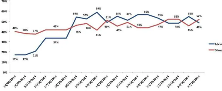
When looking at Figure 3, it becomes obvious that this electoral race was an extremely close head-to-head race with many game changing events and an unusual frequency of changes in the lead.
Figure 3: Opinion poll and first and second election round results (based on Eleições 2014. (2014,a&b))
25
This vacillation of the Brazilian voters (see Figure 3) led to great percussions within the Brazilian markets. However, it has to be academically clarified in how far this period of volatile market behaviour has been significantly related to the publication of election news. The following sections are devoted to researching this relationship.
3.1 Market Returns
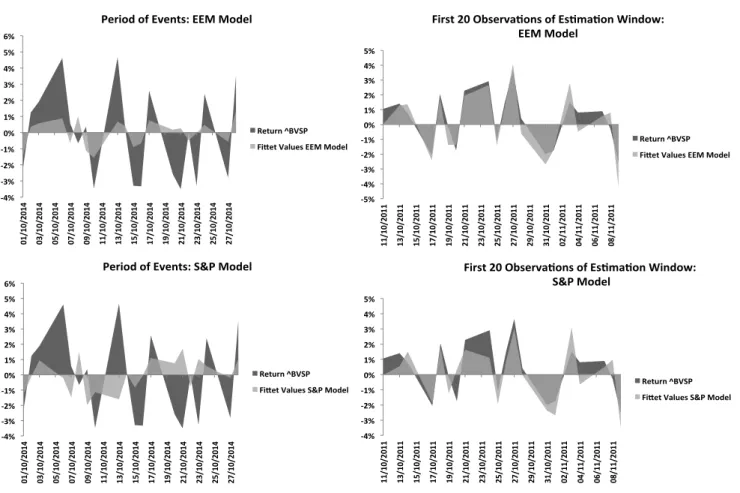
Figure 4 below shows that the fitted vales of both models fit the actual values quite well within the first twenty observations of the estimation window, see right panels of Figure 4 below.
Figure 4: Actual and fitted values: first 20 observation of Estimation Window; Period of Events26
26
It might be confusing that only 16 events are shown on the axis, this is however only due to reasons of style (size), there are indeed 20 observations represented in the graph.
!4%$ !3%$ !2%$ !1%$ 0%$ 1%$ 2%$ 3%$ 4%$ 5%$ 6%$
01/10/2014$ 03/10/2014$ 05/10/2014$ 07/10/2014$ 09/10/2014$ 11/10/2014$ 13/10/2014$ 15/10/2014$ 17/10/2014$ 19/10/2014$ 21/10/2014$ 23/10/2014$ 25/10/2014$ 27/10/2014$ Period$of$Events:$EEM$Model$ Return$^BVSP$ FiDet$Values$EEM$Model$ !5%$ !4%$ !3%$ !2%$ !1%$ 0%$ 1%$ 2%$ 3%$ 4%$ 5%$
11/10/2011$ 13/10/2011$ 15/10/2011$ 17/10/2011$ 19/10/2011$ 21/10/2011$ 23/10/2011$ 25/10/2011$ 27/10/2011$ 29/10/2011$ 31/10/2011$ 02/11/2011$ 04/11/2011$ 06/11/2011$ 08/11/2011$
First$20$ObservaIons$of$EsImaIon$Window:$ EEM$Model$ Return$^BVSP$ FiDet$Values$EEM$Model$ !4%$ !3%$ !2%$ !1%$ 0%$ 1%$ 2%$ 3%$ 4%$ 5%$ 6%$
01/10/2014$ 03/10/2014$ 05/10/2014$ 07/10/2014$ 09/10/2014$ 11/10/2014$ 13/10/2014$ 15/10/2014$ 17/10/2014$ 19/10/2014$ 21/10/2014$ 23/10/2014$ 25/10/2014$ 27/10/2014$ Period$of$Events:$S&P$Model$ Return$^BVSP$ FiDet$Values$S&P$Model$ !4%$ !3%$ !2%$ !1%$ 0%$ 1%$ 2%$ 3%$ 4%$ 5%$
11/10/2011$ 13/10/2011$ 15/10/2011$ 17/10/2011$ 19/10/2011$ 21/10/2011$ 23/10/2011$ 25/10/2011$ 27/10/2011$ 29/10/2011$ 31/10/2011$ 02/11/2011$ 04/11/2011$ 06/11/2011$ 08/11/2011$
First$20$ObservaIons$of$EsImaIon$Window:$ $S&P$Model$
When the period of events is considered, the fitted values do not fit the actual values of the Ibovespa at all, suggesting that there are in deed abnormal returns. When analysing the abnormality of returns for type I events, all four events have negative returns, and two of the four events show significant abnormal returns. On average, it has been confirmed that the returns of the four events within the category of ‘Dilma gaining in share’ have been significantly abnormal. More precisely, for both models, the null hypothesis of zero abnormal returns can be rejected with a 99% level of significance (see Table 2)27.
S&P Model EEM Model
Date R d R y Sign AR d AR y t-stat Sig
1%
Sig
5% AR d AR y t-stat
Sig 1%
Sig 5% 10/10 -3.48% -55.2% - -2.34% -37.2% -2.13 no yes -1.92% -30.5% -1.99 no yes 16/10 -3.33% -52.8% - -3.26% -51.8% -2.97 yes yes -2.67% -42.3% -2.77 yes yes 23/10 -3.29% -52.3% - -4.34% -68.9% -3.95 yes yes -3.25% -51.7% -3.38 yes yes 27/10 -2.81% -44.5% - -2.59% -41.1% -2.36 no yes -2.24% -35.5% -2.32 no yes
Ø -3.23% -51.2% -3.13% -49.8% -2.85 yes yes -2.52% -40.0% -2.62 yes yes
Table 2: Abnormal Returns Ibovespa – Type I Events
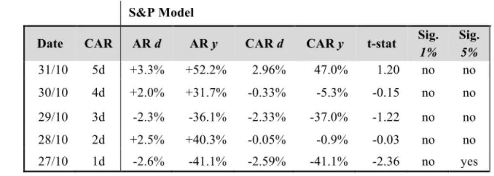
For the last event, the final election round, CARs have been calculated, see Table 3 and 4. However, none of those CARs from either model, (although having different length:
from 2 days to 5 days, see second column of Table 3 and 4 for the length), can be seen as significantly abnormal.
S&P Model
Date CAR AR d AR y CAR d CAR y t-stat Sig.
1%
Sig.
5%
31/10 5d +3.3% +52.2% 2.96% 47.0% 1.20 no no
30/10 4d +2.0% +31.7% -0.33% -5.3% -0.15 no no
29/10 3d -2.3% -36.1% -2.33% -37.0% -1.22 no no
28/10 2d +2.5% +40.3% -0.05% -0.9% -0.03 no no
27/10 1d -2.6% -41.1% -2.59% -41.1% -2.36 no yes
Table 3: CARs Ibovespa Type I Events S&P Model
27
EEM Model
Date CAR AR d AR y CAR d CAR y t-stat Sig.
1%
Sig.
5%
31/10 5d +4.0% +63.6% 3.26% 51.7% 1.51 no no
30/10 4d +1.9% +29.6% -0.75% -12.0% -0.39 no no
29/10 3d -2.6% -40.6% -2.61% -41.5% -1.57 no no
28/10 2d +2.2% +34.6% -0.06% -0.9% -0.04 no no
27/10 1d -2.2% -35.5% -2.24% -35.5% -2.32 no yes
Table 4: CARs Ibovespa Type I Events EEM Model
Due to the change of signs over consecutive trading days, the cumulative sum approaches zero at the 2-day CAR and the 4-day CAR. (Appendix 5 graphically shows the post election CARs for Ibovespa’s returns).
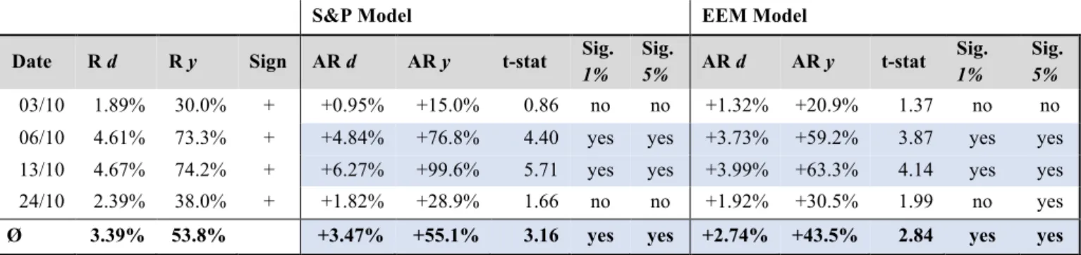
When looking at type II events, when Dilma is relatively loosing in share, all events show positive returns. There are significant abnormal returns to be found, more precisely, for two of four events, as well as for the average of all four events, the null hypothesis of zero abnormal returns can be rejected at a significance level of 99%, see Table 5 for details.
S&P Model EEM Model
Date R d R y Sign AR d AR y t-stat Sig.
1% Sig.
5% AR d AR y t-stat
Sig. 1%
Sig. 5% 03/10 1.89% 30.0% + +0.95% +15.0% 0.86 no no +1.32% +20.9% 1.37 no no 06/10 4.61% 73.3% + +4.84% +76.8% 4.40 yes yes +3.73% +59.2% 3.87 yes yes 13/10 4.67% 74.2% + +6.27% +99.6% 5.71 yes yes +3.99% +63.3% 4.14 yes yes 24/10 2.39% 38.0% + +1.82% +28.9% 1.66 no no +1.92% +30.5% 1.99 no yes
Ø 3.39% 53.8% +3.47% +55.1% 3.16 yes yes +2.74% +43.5% 2.84 yes yes
Table 5: Abnormal Returns Ibovespa – Type II Events
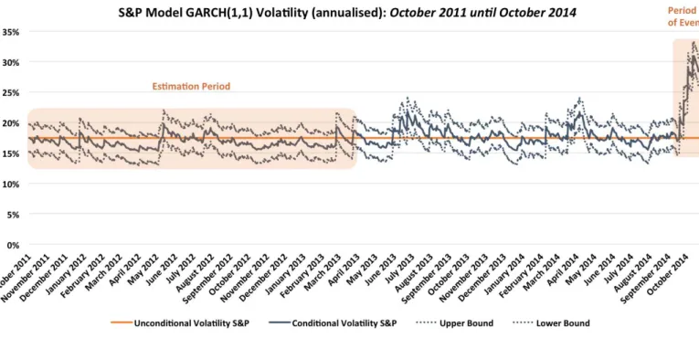
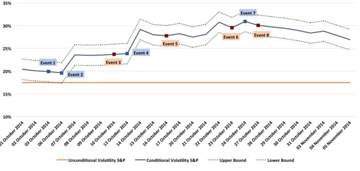
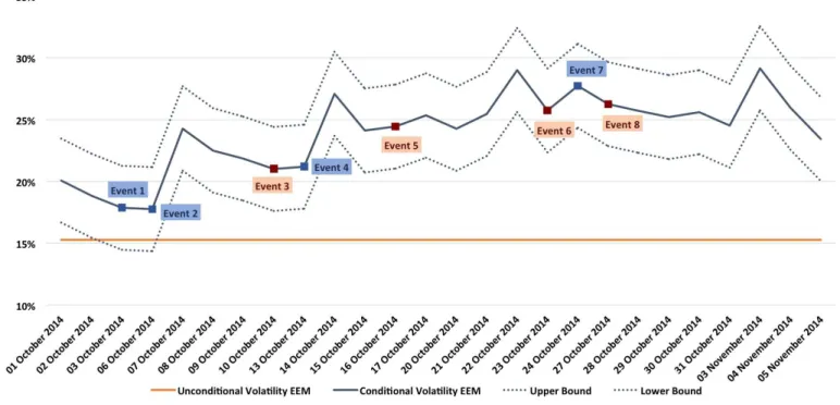
3.2 Volatility
study is looking at the entire period of events, rather than single type I and type II events, to research whether volatility is increased over the election period as a whole. Within the last section, it became obvious that during the election period returns have been switching signs very frequently, almost on a daily basis, which already implies that there should be increased volatility, when seen as the second moment of return. Due to an election period being subject to general market uncertainty, it is assumed that independent of which candidate takes the lead, at any point in time during the election period, volatility is probably increased. Ibovespa’s volatility has been proxied by the above described GARCH(1,1) model using the S&P regression’s residuals as well as the EEM regression’s residuals, see Figures 5 & 6.
Figure 6: GARCH(1,1) EEM Model annualised Volatility: Estimation Period - Period of Events
Both models show that when the election period is approaching volatility is clearly rising. Even when considering a band of ±2 standard deviations during the period of events, volatility is clearly rising far above the natural level of volatility.
Figure 8: GARCH(1,1) EEM Model annualised Volatility – Period of Events
Figure 7 and 8 display the two models’ precise evolvement of volatility during the period of events. Both models show that after October 7, Ibovespa’s volatility proxy exceeds its natural level by far, leading to a maximum annualised volatility level of 29.13% (1.84% in daily terms) within the period of events, considering data from the EEM Model28.
When conducting an event study, the graphical results can be approved. For the first two events an abnormal volatility of zero cannot be rejected, however, for the other six events, an abnormal volatility of zero can be rejected at a 99% significance level, see Appendix 4 for details.
It can be concluded that volatility reaches extremely high levels during the period of events, but slowly comes back to a normal level over time (see Figures 9 &
28
10, which show volatility in 2014 and 2015). The S&P model and the EEM model show
reversion, whereas within the EEM model, the unconditional volatility level is reached faster (after 10 trading days, precisely). Within the S&P Model approximately two month passed until abnormal volatility of zero cannot be rejected any more.
Figure 9: GARCH(1,1) S&P Model: 2014 - 2015
3.3 Volume
As already described in the modelling section, it is difficult to accurately model and forecast trading volume, therefore, a mean approach has been applied within this study. Hence, the normal level of volume, based on the mean of a 600-observation-long estimation window, is set to be approximately 3,800,000. Whereas the normal level, based on an estimation window length of 400 observations, is set to be approximately 3,400,000, (see Section 2.3.1 for the exact values).
Figure 11 and 12 below summarise the period of events of the two models. It becomes clear that trading volume in general has rather risen than decreased, since for both models the period of event average lies slightly above the estimation window averages.
Generally, the 600-observation estimation window average is higher than the 400-observation average, due to times of very high volume levels as well as variation in volume in the second half of 2013. Therefore, it follows that the slightly increased level of volume during the election period can be considered to be more abnormal when looking at the 400-obsevation average, with a lower natural level of volume.
Figure 12: Volume Ibovespa (ø 400 Obs.) – Period of Events
Based on the statistical tests below (see Table 6 and 7), it becomes obvious that, on average, there is no increased volume for Type I events, nor for Type II events.
Table 6: Abnormal Volume Ibovespa – Type I Events
ø 600 Obs. ø 400 Obs.
Date Vlm d AVlm d t-stat Sig. 1% Sig. 5% AVlm d t-stat Sig. 1% Sig. 5%
03/10 3,708,600 -87,467 -0.06 no no 291,934 0.27 no no 06/10 6,714,000 2,917,933 1.95 no no 3,297,334 3.05 yes yes 13/10 4,544,400 748,333 0.50 no no 1,127,734 1.04 no no 24/10 5,852,100 2,056,033 1.37 no no 2,435,434 2.25 no yes
øAVlm 5,204,775 1,408,708 0.94 no no 1,788,109 1.65 no no
Table 7: Abnormal Volume Ibovespa – Type II Events
However, when looking at the CAVlms after the final election day, the cumulative sum of the volume becomes significant for the 600-observation model for CAVlm(1,1) until
ø 600 Obs. ø 400 Obs.
Date Vlm d AVlm d t-stat Sig. 1% Sig. 5% AVlm d t-stat Sig. 1% Sig. 5%
10/10 3,635,700 -160,367 -0.11 no no 219,034 0.20 no no 16/10 5,427,800 1,631,733 1
.09 no no 2,011,134 1.86 no no
23/10 6,346,100 2,550,033 1.70 no no 2,929,434 2.71 yes yes 27/10 7,999,300 4,203,233 2.81 yes yes 4,582,634 4.23 yes yes
CAVlm(1,5), and stops being significantly different from zero after the 5th day. For the 400-observation model, the cumulative sum stays significantly abnormal until CAVlm(1,12); from the 13th day onwards, an hypothesis of zero abnormal returns of the cumulative sum cannot be rejected anymore. Figure 13 plots the 5-day CAVlm in its upper panel, which shows a clear upward trend; the 15-day CAVlm in the lower panel, shows that the 600-Observation Model starts to revert its cumulative sum after the 5th day; see Appendix 9 for details on the CAVlms.
3.4 Governmentally Related Stocks
3.4.1 Petrobras
The same abnormal return event study methodology that has been applied on the Ibovespa, has also been deployed on Petrobras’ common stock (Petr3.sa), as well as on its preferred version (Petr4.sa). The results are very much in line with the previous findings and even more extreme: Type I events for both stocks exhibit only negative returns. Moreover, For three out of four single type I events abnormal returns of zero can be rejected on a 99% confidence level as well as their average, for both models.
Similarly, all type II events show positive returns, with a significant abnormal average (see Appendix 6 for details on Petr3.sa and Petr4.sa’s performance). Hence, it can be concluded that Petrobras does react strongly on political news, more precisely, news regarding governmental composition.
3.4.2 Vale
Since, neither type I nor type II events yield any significant results on average, when conducting and analysing the event studies of Vale’s abnormal returns, it can be concluded that Vale’s stock did not lead to any abnormal returns during the election period. This suggests that it is not as dependent or related to governmental/ and political news as for instance Petrobras, see Appendix 7 for statistical data29.
29
4 Robustness, Further Research and Concluding Remarks
The above stated research question of whether there has been abnormal stock market behaviour as a consequence of election news regarding the last Brazilian presidential election has been confirmatively answered. The study found that there have been abnormal returns; that volatility has been significantly increased during the election period, which is in line with Bialkowski et al.’s findings (2008); and that volume was slightly elevated during the election period.
The Brazilian stock index Ibovespa, as well as the governmentally related company Petrobras, reacted with negative abnormal returns to poll releases in favour of Rousseff. When Rousseff was relatively loosing in share, there have been positive abnormal returns on the day of the release itself, or on the subsequent trading day, when the poll results have been released after market close.
In order to preclude that these abnormal values are subject to an overall South American trend, the same event study methodology was conducted on Argentina’s stock index MERVAL: As one might have expected, the results were not significant30 (see Appendix 8 for statistical data).
In order to additionally validate the study, further research on the subject may be conducted: Option strategies are one way of dealing with (electoral-) uncertainty. I.e. a straddle31, which basically bets on market movement, would be a wise strategy when considering that this research, as well as Bialkowski et al., conclude that there is an
30
On average, type I and type II events have not yielded any significant results, whereas none of the single type I events have been significantly abnormal. However, within the type II events, two single events show abnormality, whereas one of them shows a significant negative abnormal return and the second one a significant positive abnormal return. Due to differentiation in signs, other causes of abnormality are assumed.
31
overall increased level of volatility during election phases. Hence, one could look at the evolvement of option prices and underlying option strategies to further conclude about the market participants’ expectations in relation to elections.
Moreover, improvements could be made especially in regard to more accurately modelling volume. Additional governmentally related stocks, such as utilities, may also be considered to strengthen the results. Furthermore, it would be interesting to research whether there has been any abnormal behaviour in relation to foreign investment within Brazil during the election period and, consequently, in a post event window.
Another interesting evolvement can be observed when looking at the number of IPOs launched in Brazil: As Levin (2015) puts it, “these days, Brazilian companies are more likely to de-list than go public as … a crippling recession and political turmoil wipe out $290 billion in market vale this year alone” (p.1). In fact, the number of companies going public within Brazil has heavily decreased over the last two years (see Figure 14 below), a development, that may also suggest, that the political environment
does not inspire companies to go public. Within a framework of further research, it would be interesting to study the relationship of political environment and election phases and IPOs.
All in all, this study concludes that in this particular setting abnormal returns (positive as well as negative) have been possible – in this setting depending on who takes the lead. This could also be researched in an international cross-sectional setting, using for instance, Bialkowski et al.’s determinant of closeness of the electoral race. Hence, looking into elections considered to be close, and whether they reveal opposite direction of abnormal returns, more precisely, one candidate’s lead in polls is answered with positive abnormal returns while another is connected to negative abnormal returns.
Bibliography
Allvine, F., O’Neill, D. (1980). Stock Market Returns and the Presidential Election Cycle. Finacial Analysts Journal, 36(5), 49-56.
Bialkowski, J., Gootschalk, K., and Wisniewski T. P., (2008). Stock market volatility around national elections. Journal of Banking & Finance, 32, 1941–1953.
Brooks, C. (2014). Introductory econometrics for finance. (2nd Ed). Cambridge:
Cambridge University Press.
Cable, J., & Holland, K. (1999). Modelling normal returns in event studies: a
model-selection approach and pilot study. The European Journal of Finance,5(4), 331-341.
Eleições 2014. (2014,a). Resultados para Presidente do Brail (2° turno). 7Graus. Retrieved December 12, 2015, from: http://www.eleicoes2014.com.br/candidatos-presidente/
Eleições 2014. (2014,b). Pesquisa Eleeitoral para Presidente. 7Graus. Retrieved December 12, 2015, from: http://www.eleicoes2014.com.br/pesquisa-eleitoral-para-presidente/
Elliott, L. (2015). Brazil faces IPO shutdown. Financial Times, Retrieved December 11, 2015, from:
Fama, E.F. (1965). Random Walks in Stock Market Prices. Finacial Analyst Jounal, 21, 55-59.
Fama, E.F. (1970). Efficient Capital Markets: A Review of Theory and Empirical Work. Journal of Finance, 25(2), 383-417.
FES (2014). Nach der Wahl ist vor der Wahl. FES Brasilien.
Goldmann, E., Rocholl, J., and So, J. (2008). Do Politically Connected Boards Affect Firm Value?. Oxford: Oxford University Press.
G1. (2015). Juíza manda Santander indenizar demitida por texto contra Dilma. Globo, Retrieved December 12, 2015, from:
http://g1.globo.com/economia/noticia/2015/09/juiza-manda-santander-indenizar-demitida-por-texto-contra-dilma.html
Hibbs, D. (1977). Political Parties and Macroeconomic Policy. American Political Science Review. 71, 1467-1487.
Jelmayer, R., Magalhaes L. (2014). Banco Santander's Brazil Unit Fires Analyst, Others After Political Comment. The Wall Street Journal. Retrieved December 12, 2015, from:
http://online.wsj.com/articles/banco-santanders-brazil-unit-fires-analyst-others-after-political-comment-1406665764
Kothari, S. P., Warner, J. B. (2006). Econometrics of Event Studies. Centre for Corporate Governance. Tuck School of Business: Dartmouth.
Lahy, J., Pearson S. (2014). Brazil markets rally on election results. Financial Times.
Retrieved January 7, 2016, from: http://www.ft.com/intl/cms/s/0/107d2e74-4c98-11e4-a0d7-00144feab7de.html
Levin, Jonathan. (2015). Latest Symptom of Brazil’s Misery: Once-Great IPO Market Is Dead. Bloomberg, Retrieved December 13, 2015, from:
http://www.bloomberg.com/news/articles/2015-10-15/latest-symptom-of-brazil-s-misery-once-great-ipo-market-is-dead
Lucchesi, C., Hayashi, N., and Marcelino, F. (2014). Brazil’s Bankers Mute After Santander Apology to Rousseff. Bloomberg, July 30. Retrieved December 12, 2015, from: http://www.bloomberg.com/news/articles/2014-07-29/brazil-s-bankers-mute-after-santander-apology-to-rousseff
Margolis, M. (2014). Brazil Threatens Banks for Honesty. Bloomberg View, Retrieved December 12, 2015, from: http://www.bloombergview.com/articles/2014-08-01/brazil-threatens-banks-for-honesty
Medeiros, M. C., Roriz, F. (2014). Political Uncertainty and Equity Risk Premium: Evidence from the 2004 U.S. Presidential Elections. Pontifical Catholic University.
MacKinlay, A. (1997). Event Study in Economics and Finance. Journal of Economic Literature, 35(1), 13-39.
Nordhaus, W. (1975). The Political Business Cycle. Review of Economic Studies, 42, 169-190.
Pantzalis, C., Stangeland, D. and Turtle, H. (2000). Political Elections and the
Resolution of Uncertainty: The International Evidence. Journal of Banking & Finance, 42, 1575-1604.
Riley, W. B., and Luksetich, W. A. (1980). The market prefers republicans: myth or
reality. Journal of Financial and Quantitative Analysis, 15(03), 541-560.
Salomão, T. (2015). Analista do Santander demitida por projeção “polemica” recebe indenização de R$ 450 mil. InfoMoney. Retrieved December 12, 2015, from:
http://www.infomoney.com.br/mercados/politica/noticia/4278822/analista-santander-demitida-por-projecao-polemica-recebe-indenizacao-450-mil
Serra, A. P. (2002). Event Study Tests. Universidade do Porto: Porto.
Statman, M. (1999). Behaviorial finance: Past battles and future engagements.
Appendix 4 – Volatility Event study
S&P Model
EEM Model
Date ��
d �� y AV d AV y t-stat
Sig. 1%
Sig.
5% �� d �� y AV d AV y t-stat
Sig. 1%
Sig. 5% 03/10 1.25% 19.9% +0.15% +2.5% 2.18 no yes 1.13% 17.9% +0.16% +2.6% 1.53 no no 06/10 1.23% 19.6% +0.13% +2.1% 1.89 no no 1.12% 17.8% +0.16% +2.5% 1.46 no no 13/10 1.50% 23.8% +0.40% +6.4% 5.67 yes yes 1.34% 21.2% +0.37% +5.9% 3.49 yes yes 10/10 1.49% 23.7% +0.39% +6.2% 5.54 yes yes 1.32% 21.0% +0.36% +5.7% 3.38 yes yes 16/10 1.75% 27.8% +0.65% +10.3% 9.15 yes yes 1.54% 24.4% +0.58% +9.2% 5.39 yes yes 24/10 1.95% 30.9% +0.85% +13.5% 11.94 yes yes 1.62% 25.7% +0.66% +10.5% 6.16 yes yes 23/10 1.86% 29.5% +0.76% +12.1% 10.72 yes yes 1.75% 27.7% +0.78% +12.4% 7.33 yes yes 27/10 1.89% 30.0% +0.79% +12.6% 11.18 yes yes 1.65% 26.3% +0.69% +11.0% 6.46 yes yes
Ø 1.62% 25.6% +0.52% +8.2% 7.28 yes yes 1.43% 22.8% +0.47% +7.5% 4.40 yes yes
Appendix Table 1: Abnormal Volatility Ibovespa – Period of Events
Appendix Graph 1: Post-Election (15 trading days) CAV Ibovespa – after day 10 (November 11, 2014) EEM AV is not significantly abnormal anymore; CAV curve for EEM Model flattens.
Appendix 5 – Plots of Ibovespa’s post election CAR
Appendix 6 – Event study: Petrobras
S&P
Model
EEM Model
Date R d R y Sign AR d AR y t-stat Sig.
1% Sig.
5% AR d AR y t-stat
Sig. 1%
Sig. 5% 10/10 -5.99% -95.0% - -4.52% -71.7% -2.16 no yes -3.99% -63.4% -2.02 no yes 16/10 -7.53% -119.6% - -7.38% -117.1% -3.53 yes yes -6.64% -105.5% -3.36 yes yes 23/10 -6.43% -102.1% - -7.64% -121.3% -3.66 yes yes -6.31% -100.2% -3.20 yes yes 27/10 -10.96% -174.0% - -10.62% -168.6% -5.09 yes yes -10.19% -161.7% -5.15 yes yes
øAR -7.73% -122.7% -7.54% -119.7% -3.61 yes yes -6.78% -107.7% -3.43 yes yes
Appendix Table 2: Abnormal Returns Petr3.sa – Type I Events
S&P
Model
EEM Model
Date R d R y Sign AR d AR y t-stat Sig.
1% Sig.
5% AR d AR y t-stat
Sig. 1%
Sig. 5% 03/10 5.34% 84.8% + +4.26% +67.6% 2.04 no yes +4.70% +74.6% 2.38 no yes 06/10 9.27% 147.2% + +9.62% +152.7% 4.61 yes yes +8.24% +130.9% 4.17 yes yes 13/10 9.87% 156.7% + +11.91% +189.1% 5.70 yes yes +9.10% +144.4% 4.60 yes yes 24/10 4.23% 67.1% + +3.61% +57.2% 1.73 no no +3.71% +58.9% 1.88 no no
øAR 7.18% 113.9% +7.35% +116.6% 3.52 yes yes +6.44% +102.2% 3.26 yes yes
Appendix Table 3: Abnormal Returns Petr3.sa – Type II Events
S&P
Model
EEM Model
Date R d R y Sign AR d AR y t-stat Sig.
1% Sig.
5% AR d AR y t-stat
Sig. 1%
Sig. 5% 10/10 -5.58% -88.5% - -4.33% -68.8% -2.07 no yes -3.67% -58.2% -1.90 no no 16/10 -7.74% -122.8% - -7.68% -122.0% -3.68 yes yes -6.93% -110.1% -3.59 yes yes 23/10 -7.50% -119.0% - -8.68% -137.8% -4.15 yes yes -7.47% -118.5% -3.87 yes yes 27/10 -11.56% -183.6% - -11.34% -180.1% -5.43 yes yes -10.88% -172.6% -5.64 yes yes
øAR -8.09% -128.5% -8.01% -127.1% -3.83 yes yes -7.24% -114.9% -3.75 yes yes
Appendix Table 4: Abnormal Returns Petr4.sa – Type I Events
S&P
Model
EEM Model
Date R d R y Sign AR d AR y t-stat Sig.
1% Sig.
5% AR d AR y t-stat
Sig. 1%
Sig. 5% 03/10 5.89% 93.5% + +4.83% +76.6% 2.31 no yes +5.17% +82.0% 2.68 yes yes 06/10 10.54% 167.3% + +10.77% +171.0% 5.15 yes yes +9.43% +149.7% 4.89 yes yes 13/10 9.87% 156.7% + +11.64% +184.7% 5.57 yes yes +9.01% +143.1% 4.67 yes yes 24/10 5.61% 89.1% + +4.96% +78.8% 2.38 no yes +5.01% +79.6% 2.60 yes yes
øAR 7.98% 126.7% +8.05% +127.8% 3.85 yes yes +7.16% +113.6% 3.71 yes yes
Appendix 7 – Event Study: Vale
S&P
Model
EEM Model
Date R d R y Sign AR d AR y t-stat Sig.
1% Sig.
5% AR d AR y t-stat
Sig. 1%
Sig. 5% 10/10 -3.16% -50.2% - -1.26% -20.0% -0.73 no no -0.52% -8.3% -0.36 no no 16/10 -3.70% -58.7% - -3.54% -56.2% -2.06 no yes -2.55% -40.5% -1.76 no no 23/10 0.09% 1.5% + -1.55% -24.6% -0.90 no no +0.21% +3.3% 0.14 no no 27/10 -5.34% -84.7% - -4.93% -78.3% -2.86 yes yes -4.34% -68.9% -3.00 yes yes
øAR -3.03% -48.0% -2.82% -44.8% -1.64 no no -1.80% -28.6% -1.25 no no
Appendix Table 6: Abnormal Returns Vale – Type I Events
S&P
Model
EEM Model
Date R d R y Sign AR d AR y t-stat Sig.
1% Sig.
5% AR d AR y t-stat
Sig. 1%
Sig. 5% 03/10 -0.63% -10.1% - -2.11% -33.5% -1.23 no no -1.54% -24.4% -1.06 no no 06/10 2.60% 41.2% + +3.01% +47.8% 1.75 no no +1.17% +18.6% 0.81 no no 13/10 5.10% 80.9% + +7.76% +123.1% 4.51 yes yes +4.01% +63.7% 2.77 yes yes 24/10 3.00% 47.6% + +2.13% +33.9% 1.24 no no +2.26% +35.9% 1.56 no no
øAR 2.52% 39.9% +2.70% +42.8% 1.57 no no +1.48% +23.5% 1.02 no no
Appendix Table 7: Abnormal Returns Vale – Type II Events
S&P
Model
EEM Model
Date R d R y Sign AR d AR y
t-stat Sig. 1%
Sig.
5% AR d AR y t-stat
Sig. 1%
Sig. 5%
10/10 -1.80%
-28.6% - -0.99% -15.7% -0.40 no no -0.53% -8.4% -0.22 no no 16/10 -2.93% -46.4% - -2.92% -46.4% -1.16 no no -2.41% -38.3% -0.99 no no 23/10 1.88% 29.8% + +1.05% +16.7% 0.42 no no +1.87% +29.7% 0.77 no no 27/10 -4.09% -64.9% - -3.97% -63.0% -1.58 no no -3.65% -58.0% -1.49 no no
øAR -1.73% -27.5% -1.71% -27.1% -0.68 no no -1.18% -18.7% -0.48 no no
Appendix Table 8: Abnormal Returns Vale5.sa – Type I Events
S&P
Model
EEM Model
Date R d R y Sign AR d AR y t-stat Sig.
1% Sig.
5% AR d AR y t-stat
Sig. 1%
Sig. 5% 03/10 -1.70% -27.0% - -2.46% -39.0% -0.98 no no -2.23% -35.4% -0.91 no no 06/10 -0.13% -2.0% - -0.00% -0.1% 0.00 no no -0.92% -14.6% -0.38 no no 13/10 4.24% 67.3% + +5.40% +85.7% 2.15 no yes +3.62% +57.4% 1.48 no no 24/10 0.38% 6.0% + -0.09% -1.4% -0.04 no no -0.06% -1.0% -0.03 no no
øAR 0.70% 11.1% +0.71% +11.3% 0.28 no no +0.10% +1.6% 0.04 no no
Appendix 8 – Event Study Abnormal Returns: Merval (Placebo Study)
S&P
Model
EEM Model
Date R d R y Sign AR d AR y t-stat Sig.
1% Sig.
5% AR d AR y t-stat
Sig. 1%
Sig. 5% 10/10 -1.62% -25.7% - -0.66% -10.5% -0.40 no no -0.35% -5.6% -0.22 no no 16/10 3.32% 52.7% + +3.20% +50.8% 1.95 no no +3.75% +59.6% 2.35 no yes 23/10 -2.69% -42.7% - -3.92% -62.2% -2.38 no yes -2.83% -45.0% -1.77 no no 27/10 -2.50% -39.6% - -2.46% -39.1% -1.50 no no -2.15% -34.1% -1.34 no no
øAR -0.87% -13.8% -0.96% -15.2% -0.58 no no -0.39% -6.3% -0.25 no no
Appendix Table 9: Abnormal Returns Merval – Type I Events
S&P
Model
EEM Model
Date R d R y Sign AR d AR y t-stat Sig.
1% Sig.
5% AR d AR y t-stat
Sig. 1%
Sig. 5% 03/10 6.48% 102.8% + +5.36% +85.0% 3.26 yes yes +5.77% +91.6% 3.61 yes yes 06/10 -4.42% -70.2% - -4.38% -69.5% -2.67 yes yes -5.42% -86.0% -3.39 yes yes 13/10 0.00% 0.0% + -0.19% -3.0% -0.11 no no -0.16% -2.5% -0.10 no no 24/10 2.76% 43.9% + +2.02% +32.0% 1.23 no no +2.15% +34.1% 1.34 no no
øAR 1.20% 19.1% +0.70% +11.1% 0.43 no no +0.58% +9.3% 0.37 no no
Appendix Table 10: Abnormal Returns Merval – Type II Events
Appendix 9 – CAVlm Event Study
ø 600 Obs.
ø 400 Obs.
Date CAVlm Avlm d CAVlm d t-stat Sig. 1% Sig. 5% Avlm d CAVlm d t-stat Sig. 1% Sig. 5%
14/11 15d -6,767 4,437,497 0.77 no no 372,634 10,128,510 2.42 no yes 13/11 14d -763,167 4,444,264 0.79 no no -383,766 9,755,876 2.41 no yes 12/11 13d -597,467 5,207,431 0.97 no no -218,066 10,139,642 2.60 yes yes 11/11 12d -1,117,567 5,804,898 1.12 no no -738,166 10,357,708 2.76 yes yes 10/11 11d -822,367 6,922,465 1.40 no no -442,966 11,095,874 3.09 yes yes 07/11 10d -203,467 7,744,832 1.64 no no 175,934 11,538,840 3.37 yes yes 06/11 9d -103,567 7,948,298 1.77 no no 275,834 11,362,906 3.50 yes yes 05/11 8d -894,467 8,051,865 1.90 no no -515,066 11,087,072 3.62 yes yes 04/11 7d -266,267 8,946,332 2.26 no yes 113,134 11,602,138 4.05 yes yes 03/11 6d -130,867 9,212,599 2.51 no yes 248,534 11,489,004 4.33 yes yes 31/10 5d 1,552,133 9,343,466 2.79 yes yes 1,931,534 11,240,470 4.64 yes yes 30/10 4d 503,633 7,791,333 2.60 yes yes 883,034 9,308,936 4.30 yes yes 29/10 3d 1,119,233 7,287,700 2.81 yes yes 1,498,634 8,425,902 4.49 yes yes 28/10 2d 1,965,233 6,168,466 2.92 yes yes 2,344,634 6,927,268 4.53 yes yes 27/10 1d 4,203,233 4,203,233 2.81 yes yes 4,582,634 4,582,634 4.23 yes yes