FUNDAÇÃO GETULIO VARGAS ESCOLA DE ECONOMIA DE SÃO PAULO
AUGUSTO DE BARROS LISBOA DE CARVALHO
PRICING THE COST OF AN ELECTION: THE IMPACT OF THE 2014
ELECTIONS ON STOCK MARKETS
FUNDAÇÃO GETULIO VARGAS ESCOLA DE ECONOMIA DE SÃO PAULO
AUGUSTO DE BARROS LISBOA DE CARVALHO
PRICING THE COST OF AN ELECTION: THE IMPACT OF THE 2014
ELECTIONS ON STOCK MARKETS
Dissertação apresentada à Escola de Economia de São Paulo da Fundação Getulio Vargas como requisito para obtenção do título de Mestre em Economia de Empresas
Campo de Conhecimento: Macroeconomia e Finanças
Orientador: Prof. Dr. Bernardo Guimaraes
Carvalho, Augusto de Barros Lisboa de.
Pricing the cost of an election : the impact of the 2014 elections on stock markets / Augusto de Barros Lisboa de Carvalho. - 2016.
37 f.
Orientador: Bernardo de Vasconcellos Guimarães
Dissertação (mestrado) - Escola de Economia de São Paulo.
1. PETROBRÁS. 2. Eleições – Aspectos econômicos. 3. Presidentes –
Brasil - Eleições. 4. Mercado financeiro - Brasil. I. 3Guimarães, Bernardo de Vasconcellos. II. Dissertação (mestrado) - Escola de Economia de São Paulo. III. Título.
AUGUSTO DE BARROS LISBOA DE CARVALHO
PRICING THE COST OF AN ELECTION: THE IMPACT OF THE 2014
ELECTIONS ON STOCK MARKETS
Dissertação apresentada à Escola de Economia de São Paulo da Fundação Getulio Vargas como requisito para obtenção do título de Mestre em Economia de Empresas
Campo de Conhecimento: Macroeconomia e Finanças
Data de aprovação
/ /
Banca Examinadora:
Prof. Dr. Bernardo Guimaraes (Orientador) FGV-EESP
Professor Bruno Cara Giovannetti, Ph.D. USP-FEA
Professor Marcelo Fernandes, Ph.D. EESP-FGV
ABSTRACT
What is the effect of elections on real assets? Can we measure the effect on price only observing one outcome? This dissertation attempts to estimate these effects using a methodology based in stock options. The model developed adapts the benchmark Black-Scholes model to incorporate two new parameters: a perfectly anticipated jump in price (∆) and a series of daily probabilities (Θ) reflect-ing beliefs about outcomes of the election. We apply this method to 2014 Brazilian Presidential Elections and Petrobras - an important oil company in Brazil - using market data from the second election round. The results found show 65-77% difference in company valuation, depending on election outcome. This is equivalent to approximately 2.5% of Brazil’s GDP in 2014.
RESUMO
Qual o efeito de eleições em ativos reais? É possível mensurar diretamente a diferença de preços mesmo que só possamos enxergar um dos resultados potenciais? Essa dissertação estima esses efei-tos utilizando metodologia baseada em opções sobre ações. O modelo aqui desenvolvido adapta o tradicional Black-Scholes para incorporar dois novos parâmetros: um salto no preço do ativo perfei-tamente antecipado (∆) e uma série de probabilidades diárias (Θ) refletindo as crenças sobre quem venceria a corrida eleitoral. Aplicamos esse método para o caso brasileiro das Eleições Presiden-ciais de 2014 e a Petrobras - uma importante companhia do setor petrolífero do país - utilizando dados de bolsa do segundo turno das eleições. Os resultados encontrados mostram uma diferença de 65-77% para o valor da companhia, dependendo de quem vencesse nas urnas. Isso é equivalente a aproximadamente 2.5% do PIB de 2014 do país.
Contents
1 Introduction 6
1.1 Literature Review . . . 7
2 Elections and Petrobras 11
2.1 Presidential Candidates and the First Election Round . . . 11 2.2 The Second Election Round and Petrobras . . . 12 2.3 Petrobras Politics . . . 13
3 Proposed Methodology 15
3.1 Empirical Model . . . 15 3.2 Data and Estimation . . . 18 3.3 A Discussion on Identification . . . 19
4 Results 22
4.1 Robustness to Other Specifications . . . 28
5 Extension 29
5.1 The Heston model . . . 29 5.2 Estimation Results . . . 30
6 Concluding Remarks 32
A Appendix 37
6
1 Introduction
How important are elections to economic outcomes? This is the million dollar question to any-one faced with a ballot and in need to make a decision. But answering it in a precise and objective manner is not straightforward. Analyzing the election effect on asset prices is not enough to answer it since there is no counterfactual with which to compare. Additionally, it is often that election results are partially (sometimes completely) expected which makes detecting these effects increas-ingly difficult.
This dissertation proposes a method to estimate these effects and applies it to Brazil’s 2014 presidential elections. We will rely on stock options with different strikes to estimate the probability distribution of the underlying asset price under different incumbent presidents. By using market expectations to recreate the counterfactual we can compare the possible outcomes and isolate the election effect.
Our model is an extension of the original Black-Scholes (BS) with two extra elements. The first, a fixed difference parameter to be interpreted as the gap in valuation of the asset if a president had already been elected. And the second, a time series of daily probabilities reflecting the constantly changing market expectations regarding the election outcome.
We use our model to study Petrobras, the largest oil company in Brazil and a state controlled business. With increased volatility from oil prices during the period and a very close presidential race, there was plenty anecdotal evidence that the potential election outcome was affecting the company’s stock prices.
The findings reported show a difference of 65-78% in stock prices had a different president been elected. This translates to U$ 50.6-57.7 million difference in company valuation, equal to 2.1-2.5% of the country’s 2014 GDP. This price drop could reflect how the market expected the company’s future profitability in face to the elected president’s public policies, such as subsidised gas prices or local-content laws. Reported results for the election outcome probabilities are in general agree-ment to the moveagree-ments in presidential polls. Reassuringly, from the Election Day on, the estimate attributes 1 probability that the elected president would win the race.
Introduction 7
The results suggest that the election outcome indeed affected Brazil’s economic outcome. More-over, the magnitude of the estimated impact is relevant to future discussions of the country’s eco-nomic policies. The proposed methodology, however, is not limited to the Brazilian case. It could be used to analyze other close election races with potentially big economic impacts.
1.1
Literature Review
Evaluating the impact of elections and politics on real assets has been motivating several re-searchers and fueling many debates for a few decades now. The question whether or not different partisan orientations and policies affect market returns is a natural one to make, but separating the effects of economic policies from macroeconomic variables in expected returns has proven to be a hard task for researchers. The two traditional problems faced by the literature are the lack of counterfactuals, which would allow isolating policy effects from business cycles and; explain-ing economic outcome through politics is an endogenous problem by nature. Nevertheless, both theoretical models and observational studies tried to assess whether equity market “preferred low inflation right-wing governments or low unemployment policies from left-wing incumbents (see Hibbs (1977)).
Several traditional studies tried to shed light on the issue from an aggregate stock market return approach, looking for predictable cycles. Analyzing a specific period, these studies tried to match past high and low average market returns to political orientation of the incumbent president (or equivalent). In Niederhoffer et al. (1970), Allvine and O’Neill (1980) and Tufte (1980) the authors found evidence strongly suggesting the existence of a business cycle revolving the election periods in the US stock market, whereas Hensel and Ziemba (1995) showed that stocks from small-caps enjoyed higher returns during Democratic administrations. Analysis such as these cannot infer the causal nature of the cycles or market preferences (to left and right-wing governments) due to endogeneity problems and the because long periods analyzed usually span very different (and most likely not comparable) macroeconomic scenarios. Gärtner and Wellershoff (1995) expanded previous studies augmenting the estimation by using ARMA models and macroeconomic variables, arguably reducing the latter problem.
Introduction 8
higher average returns around election date and Roberts (1990) assesses the effect of expected pub-lic popub-licies in stock markets during the 1980 US general election period. Studies of how markets react to the political orientation of the winning parties of presidential elections are conducted in Santa-Clara and Valkanov (2003a) and Bialkowski et al. (2007a), for the US stock market and 23 other OECD countries, respectively.1 Leblang and Mukherjee (2005) present a theoretical model explaining how average returns and market volatility react to the elected presidents position in the political spectrum and uses the predictions to engage in an initial welfare discussion. Białkowski et al. (2008) rigorously tested and found evidence of volatility spikes during election periods in 27 OECD countries and; studies such as Jensen and Schmith (2005) and Füss and Bechtel (2008) further expand the robustness of the event-study approach by utilizing GARCH models to assess election impacts.
The event study methodology was undeniably important to the advances of the political econ-omy literature, but it has a chink in its armor. It estimates political effects in equity market assuming that, close to the analyzed event, market reacts only to political news. However, that requires ratio-nal investors to be surprised by elections results every time, otherwise the reaction would already have been priced. Although Bialkowski et al. (2007a) claimed that their results are consistent with investor surprise, an objective measurement is needed to produce an unbiased estimate of market reaction magnitudes. It is roughly at this point, amongst other studies that try to gauge the level of investor surprise given the political scenario, that this paper should be placed. Herron et al. (1999) finds that approximately a fifth of the American economic sectors significantly reacted to movements in the Iowa Electronic Market2-based measures related to the presidential race of 1992. Attempting to estimate the impact of a Bush reelection in 2004, Snowberg et al. (2007) matches high frequency financial data to the market-based probability of the candidates reelection from TradeSports.com.3The results suggests a 2-3% increase in equity prices. Our paper will approach the estimation much like these last two studies, trying to uncover election probabilities implicit in market prices, and use them to estimate the election effects.
When it comes to addressing beliefs about the future, the market could be a rich source of in-formation since prices today should reflect investors’ expectations for tomorrow. But to actually extract these beliefs from prices, the development of some tools was required. The idea that traded options carry forward-looking information and using them to extract implied probability density
1For other applications and estimates of how new legislation affected the market and the price of traded companies,
refer to Gilligan and Krehbiel (1988) and Boardman et al. (1997).
2The Iowa Electronic Markets (IEM) is a market in which traders can buy and sell securities contingent to political
election results and economic indicators. It is operated by the University of Iowa Tippie College of Business.
3Betting website that allows its users to bet on the outcome of different sports. In 2004 the website created a security
Introduction 9
functions (PDFs)4 was first explored in Breeden and Litzenberger (1978). They elegantly showed how to extract such Risk-Neutral Densities (RNDs)5 by observing the derivatives price reaction
with respect to the strike price, making no assumptions on either the underlying asset price dy-namics or on the PDF itself. This approach allow us to look at probabilities of different outcomes, something that the event study methodology usually cannot do.
Nonparametric approaches were used to infer expectations about several exchange rates in Campa et al. (1998) and Campa et al. (2002a), bond market in Germany in Söderlind and Svens-son (1997) and the S&P 500 stocks in Figlewski (2008) and Aït-Sahalia and Lo (1998).6Although
theoretically sound, extracting these probabilities non-parametrically is data-intensive,7 thus may yield poor results for illiquid markets (small samples).
An alternative way of estimating risk-neutral densities when data is limited is to impose a structure on the data generating processes: the asset price dynamic, the volatility dynamics or on the implied density itself (or, possibly, on a combination of all previous mentions). The most famous example of a parametric option pricing model is, of course, the one proposed by Black and Scholes (see Black and Scholes (1973a)), in which the geometric Brownian motion assumption of the asset price implies a log-normal density. Although arguably outdated, it is still a benchmark model in the sense that many contributions in parametric estimation are generalizations of diffusion-based models. Merton generalized the model for options of dividend paying stocks in Merton (1973), in Merton (1974) he proposed a parametric approach for bond pricing and on Merton (1976) he extends the model to accommodate jump probabilities of the underlying. In parallel, Heston (1993) and Hull and White (1987) proposed parametric models with stochastic volatility to further relax restrictive assumptions of the original Black-Scholes model.
Several applied studies relied on parametric models to approach a wide range of questions. Melino and Turnbull (1990) proposed a model to estimate foreign currency option prices whereas Malz (1996), Mizrach (1996) and Bates (1996) used similar models with jumps to estimate implied realignment probabilities of European exchange rates. Saa-Requejo and Santa-Clara (1997) studied bond pricing while Bahra (1997), Bakshi et al. (1997) and Bates (2000) (among others) inferred expectations about equity markets. Parametric models require only a small quantity of parameters
4General Equilibrium models proposed by Lucas Jr (1978) and Rubinstein (1976) will describe these PDFs as the
probabilities of possible outcomes weighted by the marginal rates of substitution for each outcome. In practice, these probability densities can be very different from an assets payoff probabilities.
5These PDFs are sometimes referred to as Risk-Neutral Densities in reference to the researchers from Christie
(1982) and Cox and Ross (1976). They assumed all investors were risk-neutral, thus all assets in such a world had to yield the risk-free return rate. That assumption can be used to derive the Black-Scholes option pricing formula.
6Further contribution to nonparametric estimation methods using probability densities to draw implied binomial
trees can be found in Dupire et al. (1994) and Rubinstein (1994), to name a few.
7As described in Breeden and Litzenberger (1978), if we could observe options with a continuous of strike prices,
Introduction 10
11
2 Elections and Petrobras
The presidential election we are about to analyze was a convoluted one: this race was the closest one since 1989, when direct elections reappeared in Brazil after over 20 years of military govern-ment. This means it was the closest election most of the Brazilian voters have seen.
The fierceness of the race was reflected by the behaviour of the candidates, the frailty of the last minute alliances formed and the overall tense political climate of the country. The constant cross-fire of graft accusations between candidates, a tragedy that reshaped the political field (Eduardo Campos incident) and heated debates in open TV: all exacerbated the uncertainty. From political warfare to candidates dancing tofunk1/Capoeira2 and attempting the ice bucket challenge3, it was
a convoluted yet fun election period.
Later on, we argue that the degree of uncertainty created by this race will greatly improve ability of our model to identify what we are looking for. Thus a quick recap of the election’s facts seems fitting, although if the reader is already acquainted to the Brazilian political scenario, feel free to skip to the next section.
2.1
Presidential Candidates and the First Election Round
In June 2014, each party officially announced their presidential candidates. Out of the 11 total canditates, we will focus on 3 specific ones since they held over 90% of the valid votes at all times: Dilma Roussef from the Worker’s Party (PT), reelection candidate with a left-wing progressive government plan; Aécio Neves from the Brazilian Social-Democratic Party (PSDB), regarded as the center-right candidate in direct opposition to the Worker’s Party and; Eduardo Campos/Marina Silva from the Brazilian Socialist Party (PSB), whom brought to the table a more legitimate social-democratic speech and were perceived as the “middle-ground” party compared to the previous two. PT’s candidate advantage to her peers was undeniable prior to the first election round, as Ms. Roussef enjoyed ratings of 40 to 50% of valid votes across all polls throughout the period.
Achiev-1Music genre with origin attributed to the slums inRio de Janeiro, hence the namefunk carioca. Not to be confused
with then American funk genre, which has influences from jazz, rhythm and blues and others.
2Martial art developed in Brazil by African descendants which combines aspects of music, dance and acrobatics. 3Campaign aiming to promote awareness of the Lou Gehrig’s Disease. Went viral in social medias during
Elections and Petrobras 12
ing the majority of valid votes would mean no second round and, on several occasions, the chances of a one-round election seemed very high.
At the same time Ms. Roussef was shooting for reelection straight from the first round and competing againsteveryone, the other two candidates were competing amongst themselves. Since
victory was impossible for them, Aécio and Marina were fighting to be Dilma’s adversary while hoping for a second round to take place. This dispute became especially uncertain when PSDB lost its six months long advantage a little over three weeks from election day.
Since the beginning of the year, polls have been published every now and then and PSDB had always held second place. Until then, it was natural to expect that the second round (if it were to happen) would present a face off between PT and PSDB. This notion drastically changed after Eduardo Campos’ tragic death in August 14th, amidst the presidential campaign. Marina Silva, PSB’s coalition vice-president candidate, stepped up to take Mr. Campos’ place as candidate for presidency and was eloquently supported. Marina held her ground against the PSDB opponent for over 2 weeks, with poll differences sometimes reaching up to 10 percentage points over Aécio. It was only two days prior to voting day that Mr. Neves overtook Ms. Silva in polls.
On election day, Dilma did not achieve majority of valid votes (41.59%) and Aécio beat Marina by a substantial margin (33.55% to 21.32%).4 The second round was going to be the stage for the
dispute between PT and PSDB and was scheduled to take place on October 26th.
2.2
The Second Election Round and Petrobras
The second round proved to be the closest presidential race since direct voting was reinstated in Brazil and. From day one, it was abundantly clear that this round wouldn’t be a repeat of the PT hegemony from the first. As expected, the majority of Marina’s voters shifted their support to the PSDB candidate during the second round. This drastically boosted Aécio’s popularity and polls from the beginning of the second round already showed the PSDB candidate slightly overtaking Dilma. During the first week of this 18 day period it looked like Aécio would take the election. At the time, this outcome took most of us by surprise since it was so disconnected from the reality seen during the period that preceded the first round.
It was only after the first week when the PT candidate started to show the favoritism seen in the first round ballots, even if only by a slight margin. This slight poll advantage did build up towards the election day, but never to a comfortable point: the average difference between the two candidates during these 10-12 days was approximately 4 percentage points. To further add to the
Elections and Petrobras 13
political noise, 2 days prior to election day a new poll result was published showing Aécio closing the gap5in the last moment of this presidential race.
On October 26ththe convoluted race came to a closing with Dilma being reelected president of Brazil, beating Aécio 51.64% to 48.36% and marking the fourth PT elected president in a row. The biggest take-away from this second period for the intents and purposes of this study is that, during the whole period, there was no clear favorite to win this race. As a matter of fact, since the error margins in polls overlapped and until the last moment, this race could have been taken by either side (both candidates were technically tied for most of the period).
2.3
Petrobras Politics
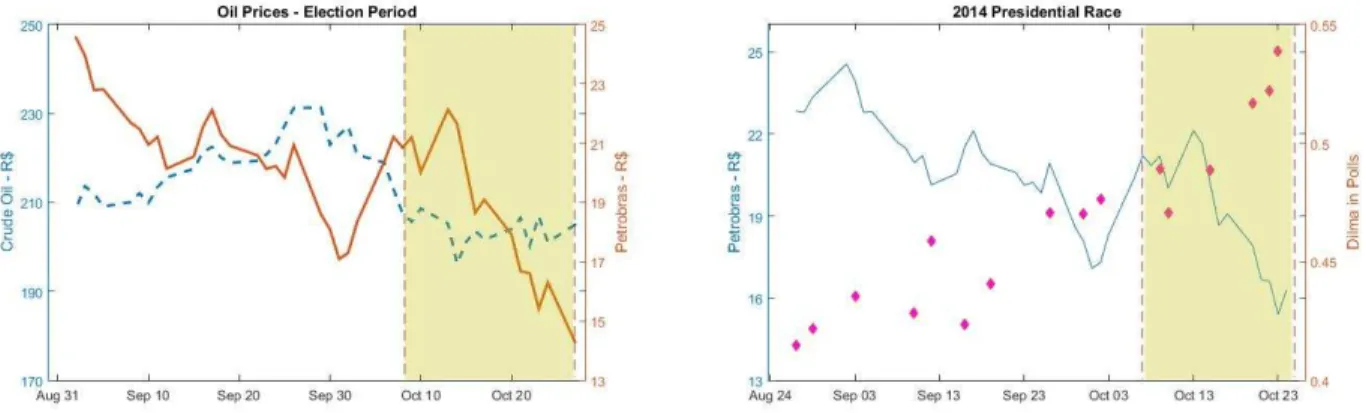
In the 2 months ranging from early September to late October of 2014, Petrobras’ stocks (BM&F: PETR46) went all the way from R$ 24.56 to R$15.28. Petrobras was created in the mid 50’s with the objective of concentrating all of the country’s oil extraction and refinement under one huge, state-owned enterprise. Fast-forwarding half a century, Petrobras was the largest company in Brazil: it is state-controlled yet listed, so part of its capital is privately held, and its net revenues exceed the R$ 330 billion mark (even no longer holding monopoly rights over the country’s oil re-serves) making it one of the most important companies for the country’s economy. So, when stock prices of such a company plummet like that, it can be quite concerning.7
Figure 1:Petrobras’ share price during the election period in contrast to the per barrel price of oil and trajectory in polls of the PT candidate. The shaded areas indicate the second round of the 2014 Presidential Elections
5Some polls released by smaller institutes actually showed Aécio overtaking Dilma during these last days prior to
ballots.
6Prefered stock with no voting rights.
7The stock currently (Feb-2016) trades at under R$ 5.00 in the Brazilian stock exchange after struggling with a
Elections and Petrobras 14
In 2014, the company faced lower than expected oil prices,8weak demand and several delays in the completion of refinement projects throughout the country. Moreover, a graft scandal9involving
Petrobras and several Brazilian politicians contributed negatively to the company’s profitability. It is clear that 2014 was far from being the best year for business. However, these were not particularly intense during the second round period. As a matter of fact, even oil prices seemed stable (Figure 1) while Petrobras’ share price fell. Whatever was affecting Petrobras doesn’t seem to be affecting
oil prices.
On the other hand, there is plenty anecdotal evidence pointing to the fact that the presidential elections also affected Petrobras’ valuation. During the first election round, the stock price reached its highest when Marina and Dilma were technically tied, and the lowest when polls showed Dilma with twice as many votes as the candidate coming in second. The biggest overnight price increase happened right after the reelection of Ms. Roussef did not materialize in the first round and the second round was confirmed. And, during the second round, the biggest price drop happened at the same time polls showed Aécio’s support starting to falter. The reason why Petrobras is so exposed to the election outcome stems from the conflict of interests intrinsic to its capital structure. As a shareholder, the government will benefit from company profits and, as a political player, it will benefit from using the company as a tool to gain political support. Since it is a state controlled business, it is completely up to the incumbent government to choose “which hat” the company will wear.
There is little that the private shareholder can do in the case of Petrobras (other than trade the stock at a higher or lower price) and his investment returns are highly correlated to the choices of the incumbent government. For example, inefficient public policies such as local-content laws and capped gas prices compromise profitability and should impact share price. Policies that a re-elected PT government seemed very inclined to keep promoting. In this sense, the market might have viewed other candidates (especially Aécio) as much less likely to intervene by promoting pub-lic popub-licies at the expense of the shareholders. Another aspect that could be affecting the market valuation of the company was political corruption, since the graft scandal that was hitting Petrobras appeared to involve the PT party to a greater degree if compared to its adversaries.
It was likely that the market valued the company very differently under different administrations. The question is, by how much?
8The year’s weak global economic growth, drastic increase in US oil production and further use of shale oil and
other substitutes are likely culprits.
9In March of the same year, the Federal Police of Brazil initiatedOperação Lava-Jato: an investigation of a money
15
3 Proposed Methodology
The next sections will describe the first model we propose. After the election in Brazil, we observed one of the potential outcomes for the presidential election (Dilma’s reelection) and the associated stock price. This model will utilize stock option prices to reconstruct the counterfactual and will focus on the second round of the Presidential Election. First, we describe the environment of the model and assumptions made, followed by the data and estimation, and close this section by discussing the identification process.
3.1
Empirical Model
To think about the impact of the second round of the presidential election we propose an econ-omy with two possible future outcomes. Each outcome associated to the victory of a specific candi-date and a valuation for the company. The existence of forward looking investors imply that before Election Day, the stock price must somehow reflect:1)the market’s valuation difference between the two outcomes and;2)the market subjective probability associated with each outcome.
Before Election Day (labeledT¯), both prices are still potential realizations. After a president is elected, only one price out of the two is chosen.
Assumption 1. For every t < T¯, there exist two potential outcomes: Sthigh and Stlow such that
Sthigh ≥Stlow, and a constant∆defined by:
∆=. S high t
Slow
t
These two values1are to be interpreted as the price that the asset would have if either president had been electedtoday(or at any other timet). Notice that the variable∆is not indexed bytand
plays the role of a proportionality constant through the whole second round. This approximation follows from the fact that voter’s expectations about each candidate’s goals and preferred policies did not significantly change in only 3 weeks. Thus, even if exogenous factors change during the
1The choice of words is purely for illustration purposes. Since no restrictions will be made to these values the result
Proposed Methodology 16
race which impact the value of the asset, these shocks will not change the relative value between the potential prices.
Assumption 2. The asset price Slow
t , without loss of generality,2 follows a Geometric Brownian
motion of the type:
dSlow
t =µS low
t dt+σS low t dWt
Additional technical assumptions are made in order to restrict ourselves to the BS environment. These are constant volatility σ during the analyzed period as well as availability of risk-free rate
financing.
The event defining which outcome is chosen is the second round election day itself and will happen at a known timeT¯. In timet < T¯, there is no perfect forecast of which president will be elected (which future state will be realized), but the market can attribute probabilitiesθtand1−θt for each outcome and update those as time passes and new information (e.g.: presidential polls, TV debates, etc.) is made available.
Assumption 3. There exists a series of probabilitiesθt, with 0 ≤ θt ≤ 1for all t < T¯), which
relate to one of the potential outcomes. These probabilities are martingale in the sense that, given
timet, we haveE[θt∗] =θt, for allt
∗
> tand independent ofS(•)
t .
Much in the spirit of Cox and Ross (1976), we will assume that agents in this economy are risk neutral. This will help in adapting BS original formula to our environment.
Assumption 4. Investors are informed about the potential outcomes and exhibit risk-neutral
be-havior. Thus, for anyt <T¯, the observed stock priceS∗
t is a probability weighted combination of
all the potential priceskgiven by
S∗ t = ∑ iθ k tS k t
Similarly to the bulk of the literature, our objective is to retrieve risk-neutral densities of the stock price during this period. As the original Black-Scholes model, we will take a parametric approach to model the price dynamic.
It follows from the definition of an European call option that today’s price of this deriva-tive C, with strike K, maturity T and given all the information I known up until today (labeled
2Notice that the price one can writeSthigh= ∆Slow
Proposed Methodology 17
C(S∗
t, K, T)) is the future expected value of this derivative brought to the present using the
risk-free rate:
C(S∗
t, K, T) =e
−∫T
t ruduE[S∗
T −K|S
∗
T ≥K, It] (1) The right-hand side of equation (1) represents what is the expected present value of the profit of holding that call option until maturity. It follows that it can be rewritten substituting the underlying asset price from Assumption 4:
E[S∗
T −K|S
∗
T ≥K, It] = E
[
θtSlow+ (1−θ)∆Slow−K
S
∗
T ≥K, It
]
=E[θt(Slow −K) S
∗
T ≥K, It
]
+
+E[(1−θt)(∆Slow−K)S
∗
T ≥K, It
]
If the maturity date of this call option is such thatT >T¯,3then one of the outcomes has already
been chosen by the time the call is exercised (in this case, the election was already won by either candidate), henceθT ={0,1}. Without loss of generality, assume thatθT = 1indicates the state in which the asset is worthSlow. Only the algebra for the first expected value operator on the previous equation is shown since the reasoning is very similar for the second one:
E[θt(Slow−K)S
∗
T ≥K, It
]
=
∫ ∞
K
θt(Slow−K)dF(S∗
T)
=
∫ ∞
K
θt(Slow−K)dF(θTSlow + (1−θT)∆Slow)
=
∫ ∞
K
θt(Slow−K)dF(Slow)
From Assumption 3,θtcan be removed from the integral. We can then repeat the previous steps for the second expected value operator and an analogous result can be found. We can use these
3Strictly speaking, convergence ofθ→1is possible beforeT¯, which would mean that the outcome of election is
Proposed Methodology 18
results and substitute them in equation (1):
C(S∗
t, K, T) =e
−∫T t rudu
[
θt
∫ ∞
K
(Slow −K)dF(Slow) +
+ (1−θt)
∫ ∞
K
(∆Slow−K)dF(∆Slow)
]
=θtC(Stlow, K, T) + (1−θt)C(S high
t , K, T) (2)
It follows that the the price of the derivative can be written as the combination of option prices associated to the potential underlying asset prices weighted by the outcome probabilities.4 Notice
that other than the probability weighting, each option price on the RHS of the previous equation can be evaluated independently using the BS formula. The results can be easily interpreted.
3.2
Data and Estimation
To estimate last section’s model we are using a data set of Petrobras’ stock options negotiated at São Paulo’s stock exchange, BM&FBovespa. In BM&FBovespa, stock options are issued once a month5 (every3rd business Monday) and issuances are identified by a capital letter (A through L for calls and M through X for puts). Issuances J/V and K/W were used in agreement to the election period and had exercise dates of Oct20th and Nov17th, respectively. Our data base counts with over 3,200 daily observations of stock option prices, strike prices as well as underlying asset prices spanning approximately 2 months (late September to mid November). We then proceed in the following way:
(i) For each observed stock option in timet, the BS formula is used to describe the derivative
priceVBS(S∗
t)as a function of each potential outcome for the underlyingS
∗
t ∈ {Stlow, S high t }:
Vi,t(low) =V BS i,t (S
low t )
Vi,t(high) =V BS i,t (S
high t )
Proposed Methodology 19
(ii) Using equation (2) and these functions, we write the theoretical option price for each
ob-served derivative:
Vth
i,t =θtVi,tBS(S low
t ) + (1−θt)V BS i,t (∆S
low t )
(iii) Assuming the theoretical price mimics the observed one (labeledVobs
i,t ), we define the error term:
ϵi,t =. Vi,tobs−Vi,tth
(iv) We minimize a non-linear sum of squares using Matlab seeking recover a scalar∆, a vector of underlying stock pricesSlow
t and a vector of probabilitiesθtfor allt <T¯: Min
∆,S,Θ
∑
iϵ
2
i
3.3
A Discussion on Identification
In the previous section we proposed a method for estimating the hypothetical parameters. Be-fore addressing the estimation itself we will use this section to elaborate on the identification mech-anism, arguing that the results we find do have economic meaning. A stock option is a particular case of a contingent claim, i.e. it is only used if a particular outcome happens and, naturally, its price depends on the probability of it being exercised. We do not observe probabilities but we do observe option prices, and their movements carry information about probabilities and expectations regarding future values of the underlying asset.6
The parameter∆is an unobserved constant andθtis a probability between 0 and 1, thus there is an infinite amount of combinations that will result in the observed price. This is why options are needed, since they carry information about different moments of the price distribution. The estimation relies on the fact that themoneynessof options and the magnitude of the∆term itself will change the way options across different strikes respond to changes in the likeliness that they will be exercised. In general terms, there are two sources of volatility in this model affecting the exercise probability of options:
1. Business as usual: new information regarding the company business, such as asset’s revalu-ation, different than expected monthly/quarterly/YTD results, success or failure of some big project, etc. This source of volatility is unrelated to the winner of the election, i.e. the failure of a project will affect the company regardless of who wins the presidential race;
6To formally prove this claim, one can differentiate twice with respect to K the integral version of equation (1) and
Proposed Methodology 20
2. Election news: new information from polls, newspapers, debates or any other media regarding candidates’ acceptance and/or chances to win. This effectively changes the probabilityθand affects observed price by giving a bigger weight to the low or high price outcomes.7
What is key for the model to estimate parameters properly is that options prices can react differently for each source of volatility.
By the means of an example, consider a put option P in our hypothetical world with strike KP such that Stlow < KP << St∗ and some unexpected good news about the increased range of applications and overall effectiveness of shale oil (“type 1” news, as previously defined). And before we proceed notice that we haveKP << Sthighwhich implies that we are implicitly assuming ∆ to be large. Petrobras extracts and refines crude oil and this unexpected news may be bad for
business so we could expectS∗
t to drop. Our put started outveryout of the money and, since∆is big, most likely we are still far from triggering our puts strike and the probability it will be exercised is still very small, thus it is still out of the money. Its price should not have moved a lot and it is still very low, which means it didnt react much to “type 1 volatility. On the other hand, if we considered a heated debate, pretty much assuring the victory of theSlow
t −candidate, then new price of our put would approachP ≈KP −Stlow. So it seemsP is very sensitive to changes inθt, namely “type 2” volatility.
We could repeat the same thought exercise in the case of smaller and smaller∆and we would notice that the options would respond less and less to “type 2 volatility and more to “type 1. This is actually very intuitive since a small∆(close to 1) means that under either president, Petrobras is valued approximately the same thus changes in chances of winning the election do not impact the stock price by a lot.8 In this case, the model is not successful in estimating any meaningful parameters. Much in the same way, an at the money option (strike price close toS∗
t) would also not be able to produce clean estimates, even if we had a large∆. Such an option would react to both types of volatility since both are likely candidates to trigger the strike price making the estimation less reliable.9
To wrap up this discussion, we would like to restate the two characteristics that will increase the quality of the estimation. The first is the existence of a large∆: the larger it is, the clearer option prices will respond to changes in the unobservable candidate election probability θt, and a close election race provided us with many opportunities to observe these movements. The second is the
7Additionally, to avoid a potential endogeneity problem, we will assume that the change in stock price itself has
minimal impact in peoples choice for president.
8The limiting case of this, when∆ = 1, impliesSlow
t =S∗t =S high
t and takes us back to the usual “Black-Scholes world.
9Even in this case the nature of the movement in price is arguably different and estimation would still be possible,
Proposed Methodology 21
moneynessof the options: out of the money options can “distinguish between the types of volatility
22
4 Results
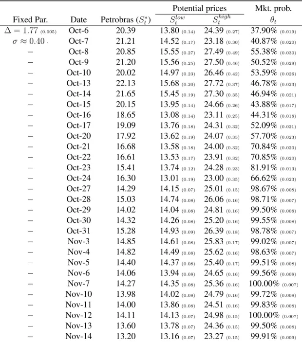
As in the BS model, stock price volatility is constant and could be either inputed or estimated. We will try both approaches. Starting by the former, the initial guess for the volatility is similar to historical averages (σ ≈ 0.40) and the probability parameters are restricted to the unit interval. Results are reported1 in Table 1 and numbers in parenthesis denote the 95% confidence interval.
Figures that follow (2 and 3) show the trajectories found for estimated parameters.
The model is capable of distinguishing between two potential outcomes, but it cannot put a nameon each one, therefore is important that we quickly address the last column of the previous
table. During the last few days the parameter was estimated to be consistently above the 70-75% mark. Moreover, after Election Day, the parameter seems to “lock” on 100.0% suggesting that there is no more doubt about who’s to be elected. According to its trajectory, we conclude that the election winner was the candidate associated to the outcomeSlow. Thus, from this point forward, we will associate the poor outcome of Petrobras to the reelection of the PT candidate, Ms. Roussef.
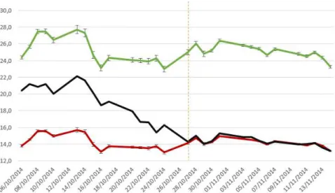
Figure 2:Estimated potential outcomes for Petrobras during the 2014 Brazilian presidential election. Historical volatility. Favorable outcome (green), least favorable outcome (red) and observed price (black). Dashed line indicates
first trading day after Election Day.
This interpretation forθtseems to be a reasonable assumption. Its trajectory depicts very well the political climate in Brazil (figure 2). Some of the movements in this series seem to relate closely to how the presidential race developed and are worth mentioning. The probability of reelection
Results 23
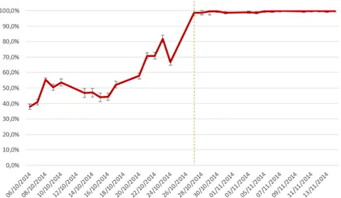
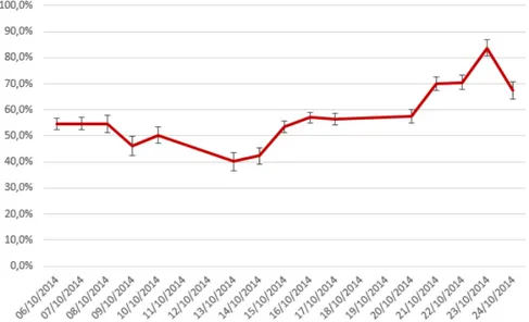
Figure 3:Estimated market probability of Dilma’s reelection. Historical volatility. Dashed line indicates first trading day after Election Day.
starts out low due to the last minute response from Aécio (PSDB) in the first round, preventing Dilma from taking the race then. A week into the second round, Dilma builds up electoral strength, taking the race through a highly uncertain couple of weeks until effectively surpassing Aécio in polls and taking the lead for the rest of the period. As the second round comes closer to an end, it seems more and more likely that Ms. Roussef was going to take the race. The last “dip” in the series reflect poll results published a couple of days prior to the election day, showing Aécio in the lead and impacting the “market certainty” of reelection. Finally, reaching the 100.0% mark and not moving, indicates the model is capturing that the election was over, and Dilma won.
We estimate that the market valued the company at a discount of approximately 77.0% (figure 3) under a PT incumbent president. This difference in price multiplied for the 13.0+ billion out-standing company shares (across ordinary and preferential shares), translates into anElection Cost
of approximately R$ 150.8 billion (equivalent to U$ 60.9 billion using Oct−27th FX rate). There are two important points to be made about this result. First, the number itself is surprising. To put it in perspective, it corresponds to roughly the market value of a Bradesco, one of the biggest banks in the country2. Second, this result is very different from previous studies that found not more than single digit percentage differences in returns for large-capitalization stocks, if any at all (see Santa-Clara and Valkanov (2003b) and Bialkowski et al. (2007b), respectively).
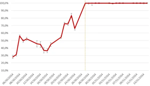
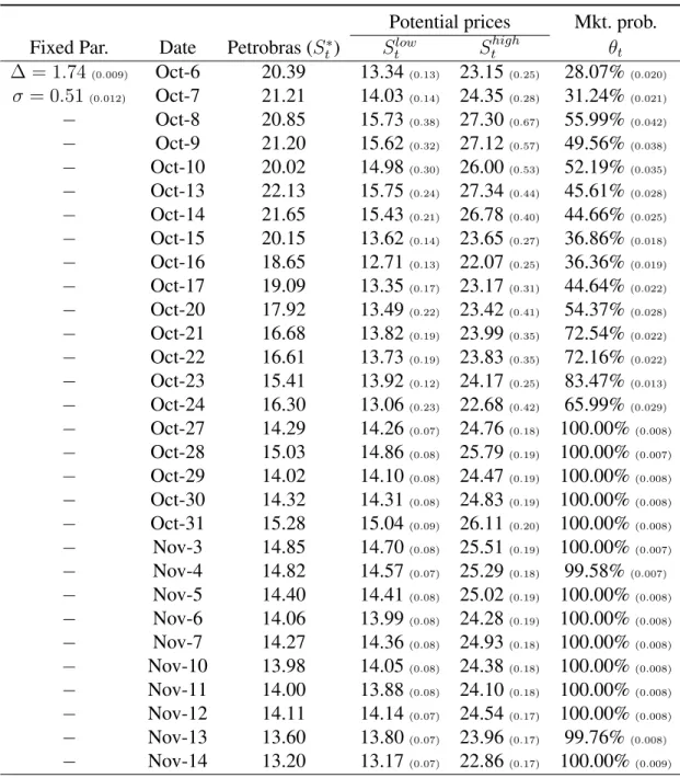
Estimating the model with a free, constant volatility parameter returns similar findings. Results are shown3 in Table 2 and numbers in parenthesis denote the 95% confidence interval. Figures 4 and 5 show the graphs for these estimates.
2Please refer to the appendix to a comprehensive list ofThings we can compare to the Cost the of 2014s Election.
Results 24
Each potential value for the underlying was estimated separately and the potential outcomes can be interpreted as independent assets. As in the original BS model, the price for each of these “assets” follow a log-normal distribution with known variance and mean (Slow
t and S high
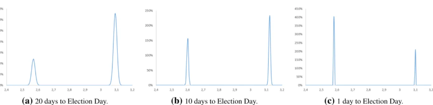
t , respectively). Thus, for any time t in our sample, we can draw two risk-neutral densities of the exercise day simply by multiplying the daily variance by the number of days to exercise. By weighting the densities byθt and(1−θt)and adding them together, we recover the risk-neutral density for the future price of Petrobras. The recovered densities are shown in figure 6.
Figure 4:Estimated potential outcomes for Petrobras during the 2014 Brazilian presidential election. Estimated (free) volatility. Favorable outcome (green), least favorable outcome (red) and observed price (black). Dashed line indicates
first trading day after Election Day.
Figure 5:Estimated market probability of Dilma’s reelection. Estimated (free) volatility. Dashed line indicates first trading day after Election Day.
Results 25
(a)20 days to Election Day. (b)10 days to Election Day. (c)1 day to Election Day.
Figure 6:Recovered risk-neutral densities for the future price (log) of Petrobras at Election Day. Free (estimated)
volatility. Distributions’ variance increase with numbers of days until election.
Results 26
Table 1:Parameter estimates using historical volatility.
Potential prices Mkt. prob. Fixed Par. Date Petrobras (S∗
t) Stlow S high
t θt
∆ = 1.77(0.005) Oct-6 20.39 13.80(0.14) 24.39(0.27) 37.90%(0.019)
σ ≈0.40- Oct-7 21.21 14.52(0.17) 23.18(0.30) 40.87%(0.020) − Oct-8 20.85 15.55(0.27) 27.49(0.49) 55.38%(0.030)
− Oct-9 21.20 15.56(0.25) 27.50(0.46) 50.52%(0.029) − Oct-10 20.02 14.97(0.23) 26.46(0.42) 53.59%(0.026) − Oct-13 22.13 15.68(0.20) 27.72(0.37) 46.78%(0.023)
− Oct-14 21.65 15.45(0.19) 27.30(0.35) 46.94%(0.021) − Oct-15 20.15 13.95(0.14) 24.66(0.26) 43.88%(0.017) − Oct-16 18.65 13.08(0.14) 23.11(0.25) 44.31%(0.018)
− Oct-17 19.09 13.76(0.18) 24.31(0.32) 52.09%(0.021) − Oct-20 17.92 13.62(0.19) 24.07(0.35) 57.70%(0.023) − Oct-21 16.68 13.58(0.18) 24.00(0.32) 70.84%(0.020)
− Oct-22 16.61 13.53(0.17) 23.91(0.32) 70.85%(0.020) − Oct-23 15.41 13.74(0.12) 24.28(0.23) 81.91%(0.013) − Oct-24 16.30 13.01(0.19) 23.00(0.35) 66.62%(0.023)
− Oct-27 14.29 14.15(0.07) 25.01(0.15) 98.67%(0.008) − Oct-28 15.03 14.74(0.08) 26.06(0.16) 98.71%(0.007) − Oct-29 14.02 14.04(0.08) 24.81(0.16) 99.50%(0.008)
− Oct-30 14.32 14.26(0.08) 25.20(0.16) 99.55%(0.008) − Oct-31 15.28 14.93(0.09) 26.39(0.18) 98.78%(0.007) − Nov-3 14.85 14.61(0.08) 25.83(0.17) 99.02%(0.007)
− Nov-4 14.82 14.49(0.08) 25.62(0.16) 98.63%(0.007) − Nov-5 14.40 14.37(0.08) 25.40(0.17) 99.51%(0.008) − Nov-6 14.06 13.94(0.08) 24.65(0.16) 99.56%(0.008)
− Nov-7 14.27 14.35(0.08) 25.36(0.16) 100.00%(0.007) − Nov-10 13.98 14.02(0.08) 24.79(0.16) 99.72%(0.008) − Nov-11 14.00 13.86(0.08) 24.51(0.16) 99.83%(0.008)
Results 27
Table 2:Parameter estimates using free volatility.
Potential prices Mkt. prob. Fixed Par. Date Petrobras (S∗
t) Stlow S high
t θt
∆ = 1.74(0.009) Oct-6 20.39 13.34(0.13) 23.15(0.25) 28.07%(0.020)
σ = 0.51(0.012) Oct-7 21.21 14.03(0.14) 24.35(0.28) 31.24%(0.021) − Oct-8 20.85 15.73(0.38) 27.30(0.67) 55.99%(0.042)
− Oct-9 21.20 15.62(0.32) 27.12(0.57) 49.56%(0.038) − Oct-10 20.02 14.98(0.30) 26.00(0.53) 52.19%(0.035) − Oct-13 22.13 15.75(0.24) 27.34(0.44) 45.61%(0.028)
− Oct-14 21.65 15.43(0.21) 26.78(0.40) 44.66%(0.025) − Oct-15 20.15 13.62(0.14) 23.65(0.27) 36.86%(0.018) − Oct-16 18.65 12.71(0.13) 22.07(0.25) 36.36%(0.019)
− Oct-17 19.09 13.35(0.17) 23.17(0.31) 44.64%(0.022) − Oct-20 17.92 13.49(0.22) 23.42(0.41) 54.37%(0.028) − Oct-21 16.68 13.82(0.19) 23.99(0.35) 72.54%(0.022)
− Oct-22 16.61 13.73(0.19) 23.83(0.35) 72.16%(0.022) − Oct-23 15.41 13.92(0.12) 24.17(0.25) 83.47%(0.013) − Oct-24 16.30 13.06(0.23) 22.68(0.42) 65.99%(0.029)
− Oct-27 14.29 14.26(0.07) 24.76(0.18) 100.00%(0.008) − Oct-28 15.03 14.86(0.08) 25.79(0.19) 100.00%(0.007) − Oct-29 14.02 14.10(0.08) 24.47(0.19) 100.00%(0.008)
− Oct-30 14.32 14.31(0.08) 24.83(0.19) 100.00%(0.008) − Oct-31 15.28 15.04(0.09) 26.11(0.20) 100.00%(0.008) − Nov-3 14.85 14.70(0.08) 25.51(0.19) 100.00%(0.007)
− Nov-4 14.82 14.57(0.07) 25.29(0.18) 99.58%(0.007) − Nov-5 14.40 14.41(0.08) 25.02(0.19) 100.00%(0.008) − Nov-6 14.06 13.99(0.08) 24.28(0.19) 100.00%(0.008)
− Nov-7 14.27 14.36(0.08) 24.93(0.18) 100.00%(0.008) − Nov-10 13.98 14.05(0.08) 24.38(0.18) 100.00%(0.008) − Nov-11 14.00 13.88(0.08) 24.10(0.18) 100.00%(0.008)
Results 28
4.1
Robustness to Other Specifications
Before closing this section, we would like to elaborate on the volatility assumption. The con-stant volatility used in our model is a strong assumption, and likely does not hold in practice. However we will argue that it may be, at least, a good enough approximation.
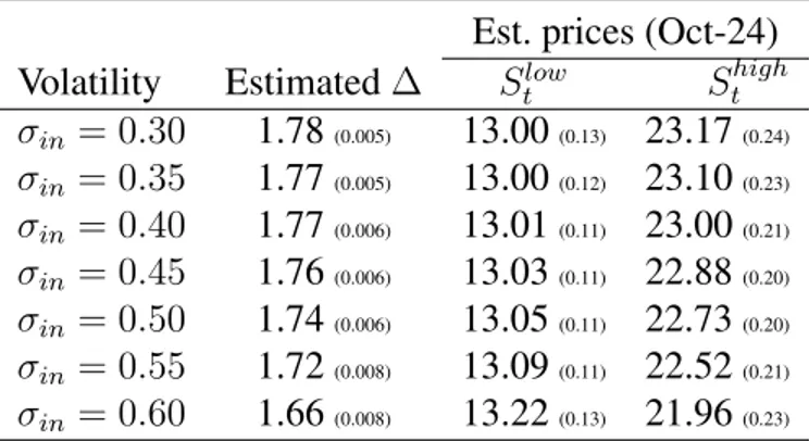
In the previous estimation, we took two approaches to estimate the parameters of interest: using inputed historical volatility and simultaneously estimating a volatility parameter. The choice of approach impacted our findings, even if just by a small amount. Trying to address the magnitude of this potential bias, we estimated the model inputting a range of different values for volatility. Their choice was oriented by observation of the past and the electoral period itself. The values chosen cover a wide, yet “reseonable” range, in which to evaluate the parameters of interest. Results are shown in table 3.
Table 3:Robustness to other values of inputed volatility.
Est. prices (Oct-24) Volatility Estimated∆ Slow
t S
high t
σin= 0.30 1.78(0.005) 13.00(0.13) 23.17(0.24)
σin= 0.35 1.77(0.005) 13.00(0.12) 23.10(0.23) σin= 0.40 1.77(0.006) 13.01(0.11) 23.00(0.21) σin= 0.45 1.76(0.006) 13.03(0.11) 22.88(0.20)
29
5 Extension
While the Black-Scholes model is the benchmark model for option pricing, it’s restrictive as-sumptions create some biases that limit how well it fits real data (see Rubinstein (1985)). The constant volatility assumption has always been frowned upon and in our case, it did affect the re-sults. The uncertain moment the company was going through could further increase this reported bias, jeopardizing the estimation. It felt natural to extend our estimation using a stochastic volatility assumption to verify if the results would still hold.
5.1
The Heston model
In his 1983 paper, Heston provided a closed form solution for option prices when the volatility parameter itself is assumed to follow a diffusion process. A call optionCHespriced by the Heston model, with underlying volatility√
v(t), strikeK and maturityT looks like:
CtHes(S
∗
t, v, T) =S
∗
tP1−K(t, T)P2 (3)
The formula shown above for a call option is guessed in analogy to the original Black-Scholes model. ParametersP1andP2are cumulative probabilities that change with respect to the moneyness
of the option. We still have to incorporate our own assumptions about the stock price, i.e. the existence of a∆and a vector of probabilitiesΘ. In the previous section we showed how the BS model can be adapted to reflect our own hypothesis. In similar fashion, we will write the solution for the theoretical call option with stochastic volatility as:
Ctth(S
∗
t, v, T) =θtCtHes(S low
t , v, T) + (1−θt)C
Hes t (S
high
t , v, T) (4)
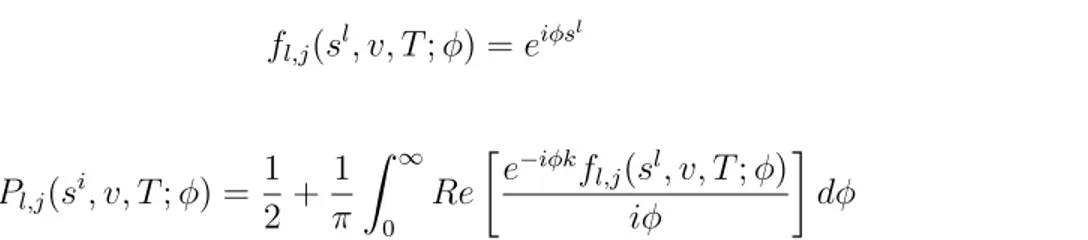
Extension 30
fl,j(sl, v, T;ϕ) = eiφsl
(5)
Pl,j(si, v, T;ϕ) = 1 2+
1
π
∫ ∞
0
Re
[
e−iφk
fl,j(sl, v, T;ϕ)
iϕ
]
dϕ (6)
Just like in the original model, we can find the solution for the price of a call option from equations (3), (5) and (6). The theoretical price is calculated by substituting the call prices just found in equation (4). The price for the put can be recovered from the put-call parity. Definition of the error term as well as the estimation process are similar to the previous section.
5.2
Estimation Results
We used the same sample of stock options as our first estimate of the adapted BS model. The objective is to guarantee results comparability. The results are reported in table 41 and trajectories depicted in figures 7 and 8.
Figure 7:Estimated potential outcomes for Petrobras during the 2014 Brazilian presidential election. Stochastic volatility. Favorable outcome (green), least favorable outcome (red) and observed price (black).
The simple BS model could be under-equipped to deal with the period’s high volatility and this could lead us to detect misleading effects. Hence the motivation to apply Heston’s model. However, the previously detected effect is still present and very significant, even in the presence of a more robust structure.
Extension 31
Figure 8:Estimated market probability of Dilma’s reelection. Stochastic volatility.
Table 4:Parameter estimates using stochastic volatility.
Potential prices Mkt. prob. Vol. Fixed Par. Date Petr (S∗
t) Stlow S high
t θt
√
v(t) ∆ = 1.65 Oct-6 20.39 15.77 26.07 54.53% 0.03
− Oct-7 21.21 16.32() 26.98 54.76% 0.26
− Oct-8 20.85 16.03 26.49 54.63% 0.69
− Oct-9 21.20 15.82 26.14 46.21% 0.70
− Oct-10 20.02 15.27 25.24 50.31% 0.67
− Oct-13 22.13 15.83 26.16 40.27% 0.72
− Oct-14 21.65 15.77 26.06 42.40% 0.66
− Oct-15 20.15 15.38 25.42 53.49% 0.37
− Oct-16 18.65 14.65 24.21 57.12% 0.28
− Oct-17 19.09 14.69 24.27 56.49% 0.48
− Oct-20 17.92 14.13 23.35 57.61% 0.61
− Oct-21 16.68 13.86 22.91 69.86% 0.61
− Oct-22 16.61 13.87 22.92 70.55% 0.65
− Oct-23 15.41 14.10 23.30 83.62% 0.67
− Oct-24 16.30 13.46 22.24 67.41% 0.78
32
6 Concluding Remarks
In Economics, more often than not, objective analysis of a problem is hindered by the lack of counterfactual evidence. The case of Presidential Elections and how its outcome influences eco-nomic output is a simple yet traditional example of such. This dissertation developed a method to approachs this problem. By extracting information about the potential outcomes from the probabil-ity densities embeded in stock options prices, we attempt to recreate the counterfactual evidence. We can compare this estimate with the realized outcome to infer the impact.
Although our focus has been on presidential races, this empirical model relies only on the assumption that agents are informed about general potential outcomes and will act accordinly. This framework is not limited to politics and can be used to estimate the impact on financial markets of other, more general, binary and perfectly anticipated events.
We have applied this methodology to the Brazilian case of the 2014 Presidential Elections and found 65-77% difference in value for Petrobras, conditional on election results. These results are surprising. The magnitude of the effect estimated is very different (larger) from what has usually been found by studies addressing similar questions, but using other methods. In particular, the intense variability of the Brazilian presidential race, caused stock options to drastically move in and out of the money and this contributed to the precision of our estimates.
33
Bibliography
Aït-Sahalia, Y. and Lo, A. W. (1998). Nonparametric estimation of state-price densities implicit in financial asset prices. The Journal of Finance, 53(2):499–547.
Allvine, F. C. and O’Neill, D. E. (1980). Stock market returns and the presidential election cycle: Implications for market efficiency. Financial Analysts Journal, 36(5):49–56.
Bahra, B. (1997). Implied risk-neutral probability density functions from option prices: theory and application.
Bakshi, G., Cao, C., and Chen, Z. (1997). Empirical performance of alternative option pricing models. The Journal of finance, 52(5):2003–2049.
Bates, D. S. (1991a). The crash of’87: Was it expected? the evidence from options markets. The journal of finance, 46(3):1009–1044.
Bates, D. S. (1991b). The crash of’87: Was it expected? the evidence from options markets.Journal of Finance, pages 1009–1044.
Bates, D. S. (1996). Jumps and stochastic volatility: Exchange rate processes implicit in deutsche mark options. Review of financial studies, 9(1):69–107.
Bates, D. S. (2000). Post-’87 crash fears in the s&p 500 futures option market. Journal of Econo-metrics, 94(1):181–238.
Bialkowski, J., Gottschalk, K., and Wisniewski, T. P. (2007a). Political orientation of government and stock market returns. Applied Financial Economics Letters, 3(4):269–273.
Bialkowski, J., Gottschalk, K., and Wisniewski, T. P. (2007b). Political orientation of government and stock market returns. Applied Financial Economics Letters, 3(4):269–273.
Białkowski, J., Gottschalk, K., and Wisniewski, T. P. (2008). Stock market volatility around na-tional elections. Journal of Banking & Finance, 32(9):1941–1953.
Black, F. and Scholes, M. (1973a). The pricing of options and corporate liabilities. The journal of political economy, pages 637–654.
Black, F. and Scholes, M. (1973b). The pricing of options and corporate liabilities. The journal of political economy, pages 637–654.
Boardman, A., Vertinsky, I., and Whistler, D. (1997). Using information diffusion models to es-timate the impacts of regulatory events on publicly traded firms. Journal of Public Economics,
BIBLIOGRAPHY 34
Breeden, D. T. and Litzenberger, R. H. (1978). Prices of state-contingent claims implicit in option prices. Journal of business, pages 621–651.
Campa, J. M., Chang, P. K., and Refalo, J. F. (2002a). An options-based analysis of emerging market exchange rate expectations: Brazil’s real plan, 1994–1999. Journal of Development Eco-nomics, 69(1):227–253.
Campa, J. M., Chang, P. K., and Refalo, J. F. (2002b). An options-based analysis of emerging market exchange rate expectations: Brazil’s real plan, 1994–1999. Journal of Development Eco-nomics, 69(1):227–253.
Campa, J. M., Chang, P. K., and Reider, R. L. (1998). Implied exchange rate distributions: evidence from otc option markets. Journal of International Money and Finance, 17(1):117–160.
Chittenden, W., Jensen, G. R., and Johnson, R. R. (1999). Presidential politics, stocks, bonds, bills, and inflation. Journal of Portfolio Management, 26(1):27–32.
Christie, A. A. (1982). The stochastic behavior of common stock variances: Value, leverage and interest rate effects. Journal of financial Economics, 10(4):407–432.
Cox, J. C. and Ross, S. A. (1976). The valuation of options for alternative stochastic processes.
Journal of financial economics, 3(1-2):145–166.
Dupire, B. et al. (1994). Pricing with a smile. Risk, 7(1):18–20.
Figlewski, S. (2008). Estimating the implied risk neutral density.
Füss, R. and Bechtel, M. M. (2008). Partisan politics and stock market performance: The effect of expected government partisanship on stock returns in the 2002 german federal election. Public Choice, 135(3-4):131–150.
Gärtner, M. and Wellershoff, K. W. (1995). Is there an election cycle in american stock returns?
International Review of Economics & Finance, 4(4):387–410.
Gilligan, T. W. and Krehbiel, K. (1988). Complex rules and congressional outcomes: An event study of energy tax legislation. The Journal of Politics, 50(03):625–654.
Hensel, C. R. and Ziemba, W. T. (1995). United states investment returns during democratic and republican administrations, 1928-1993. Financial Analysts Journal, 51(2):61–69.
Herbst, A. F. and Slinkman, C. W. (1984). Political-economic cycles in the us stock market. Finan-cial Analysts Journal, 40(2):38–44.
Herron, M. C., Lavin, J., Cram, D., and Silver, J. (1999). Measurement of political effects in the united states economy: a study of the 1992 presidential election.Economics & Politics, 11(1):51–
81.
BIBLIOGRAPHY 35
Hibbs, D. A. (1977). Political parties and macroeconomic policy.American political science review,
71(04):1467–1487.
Hull, J. and White, A. (1987). The pricing of options on assets with stochastic volatilities. The journal of finance, 42(2):281–300.
Jensen, N. M. and Schmith, S. (2005). Market responses to politics the rise of lula and the decline of the brazilian stock market. Comparative Political Studies, 38(10):1245–1270.
Leblang, D. and Mukherjee, B. (2005). Government partisanship, elections, and the stock market: examining american and british stock returns, 1930–2000.American Journal of Political Science,
49(4):780–802.
Lucas Jr, R. E. (1978). Asset prices in an exchange economy. Econometrica: Journal of the Econometric Society, pages 1429–1445.
Malz, A. M. (1996). Using option prices to estimate realignment probabilities in the european mon-etary system: the case of sterling-mark.Journal of International Money and Finance, 15(5):717–
748.
Melino, A. and Turnbull, S. M. (1990). Pricing foreign currency options with stochastic volatility.
Journal of Econometrics, 45(1):239–265.
Merton, R. C. (1973). Theory of rational option pricing. The Bell Journal of economics and
management science, pages 141–183.
Merton, R. C. (1974). On the pricing of corporate debt: The risk structure of interest rates. The Journal of finance, 29(2):449–470.
Merton, R. C. (1976). Option pricing when underlying stock returns are discontinuous. Journal of financial economics, 3(1-2):125–144.
Mizrach, B. (1996). Did option prices predict the erm crises? Technical report, Working Papers, Department of Economics, Rutgers, The State University of New Jersey.
Niederhoffer, V., Gibbs, S., and Bullock, J. (1970). Presidential elections and the stock market.
Financial Analysts Journal, pages 111–113.
Pantzalis, C., Stangeland, D. A., and Turtle, H. J. (2000). Political elections and the resolution of uncertainty: the international evidence. Journal of banking & finance, 24(10):1575–1604.
Roberts, B. E. (1990). Political institutions, policy expectations, and the 1980 election: a financial market perspective. American Journal of Political Science, pages 289–310.
Rose, A. K. and Svensson, L. E. (1994). European exchange rate credibility before the fall.
Euro-pean Economic Review, 38(6):1185–1216.
BIBLIOGRAPHY 36
Rubinstein, M. (1985). Nonparametric tests of alternative option pricing models using all reported trades and quotes on the 30 most active cboe option classes from august 23, 1976 through august 31, 1978. The Journal of Finance, 40(2):455–480.
Rubinstein, M. (1994). Implied binomial trees. The Journal of Finance, 49(3):771–818.
Saa-Requejo, J. and Santa-Clara, P. (1997). Bond pricing with default risk. Finance.
Santa-Clara, P. and Valkanov, R. (2003a). The presidential puzzle: Political cycles and the stock market. The Journal of Finance, 58(5):1841–1872.
Santa-Clara, P. and Valkanov, R. (2003b). The presidential puzzle: Political cycles and the stock market. Journal of Finance, pages 1841–1872.
Snowberg, E., Wolfers, J., and Zitzewitz, E. (2007). Partisan impacts on the economy: evidence from prediction markets and close elections. Quarterly Journal of Economics, 122(2):807–829.
Söderlind, P. and Svensson, L. (1997). New techniques to extract market expectations from finan-cial instruments. Journal of Monetary Economics, 40(2):383–429.
37
A Appendix
A.1
Comprehensive list of comparisons
Table 5:Things we can compare to the Cost of the 2014s Election. Values indicated in Reais from 2014, unless stated otherwise.
Things Worth Cost of Election equivalent to
Barrel of oil -Oct-24 201.05 746,070,000
barrels of crude oil
Brazil’s GDP 5,918tn 2.53%
of the year’s production
Average Mercosul’s GDP 1.51tn 9.9%
of the year’s production
Luxembourg’s GDP 1.52bn 101%
of the year’s production
Bradesco Bank 144.5bn 1.01
private national banks
Programa Bolsa Família 27.0bn 5.5
years of cash transfers
EESP M.Sc scholarships 36.0k 4.16mn
master program’s students
Booking your favorite band 350k to3,0mn 25,580 private concerts
Funds raised to charity in U2 concert 6.7mn 21,500 U2 fund raising events
Anticipated soccer match in Brazil 14.7mn 10,190
Corinthians’ games combined revenues
World Cup in Brazil 8.33bn 217.2