Evidence on the Incentive Properties of Share
Contracts
Luís H. B. Braido
∗University of Chicago
February 18, 2002
Abstract
Ever since Adam Smith, economists have argued that share contracts do not provide proper incentives. This paper uses tenancy data from India to assess the existence of missing incentives in this classical example of moral hazard. Sharecroppers are found to be less productive than owners, but as productive as fixed-rent tenants. Also, the productivity gap between owners and both types of tenants is driven by sample-selection issues. An endogenous selection rule matches tenancy contracts with less-skilled farmers and lower-quality lands. Due to complementarity, such a matching affects tenants’ input choices. Controlling for that, the contract form has no effect on the expected output. Next, I explicitly model farmer’s optimal decisions to test the existence of non-contractible inputs being misused. No evidence of missing incentives is found.
Keywords: econometric test, agency theory, moral hazard, tenancy data, selection bias. JEL Classification: C52, D82, O12, Q15.
1
Introduction
Moral hazard is the term used to describe situations where individuals change non-contractible behaviors in response to changes in their personal insurance. The-oretical modeling of those situations is one of the most active areas of research in economics, and many mathematical models have been in dispute for the pro-fession’s attention. The models vary from the standard textbook case with one principal, one agent, and two possible levels of effort, to more complex scenar-ios with intertemporal features (Townsend, 1982), random devices (Prescott and Townsend, 1984), double-sided incentives (Bhattacharyya and Lafontaine, 1995), and non-exclusive relationships (Bisin and Guaitoli, 2000, and Braido, 2001).
In spite of the elegance of using mathematical tools to model human behavior, the beauty of that is mostly due to the possibility of performing empirical tests. This paper uses tenancy data from India, collected by the International Crops Research Institute for Semi-Arid Tropics (ICRISAT), to empirically assess the existence of missing incentives in one of the classical examples of moral hazard: the landlord-tenant relationship.
Consider a situation where a landlord (principal) hires a tenant (agent) to manage a farm. The level of effort exerted by the tenant is unobservable and affects the farm’s expected output. Since agricultural activities are subject to random shocks (such as climatic changes and plagues), it is not possible to infer the tenant’s dedication by the farm’s outcome. Therefore, the landlord must provide incentives to induce the tenant to voluntarily choose a desirable level of effort. The theoretical literature argues that the ideal compensation contract must provide incentives by making the tenant’s salary conditional on the farm’s output.
Farms are usually cropped under three basic contract forms: ownership (where the plot is cropped by its owner); fixed-rent tenancy (where the tenant pays an upfront rent and collect the entire revenue); and sharecropping tenancy (where the landlord supplies the land, the tenant bears the costs of labor and non-labor inputs, and they share the output).1 Owners and fixed-rent tenants bear the marginal costs and receive the marginal benefit of their actions. Therefore, their plots must achieve the maximum expected output. Share contracts balance effort incentives and risk sharing (i.e., the landlord insure tenants at the cost of reducing effort incentives). Consequently, sharecropped farms would tend to be less productive than those owned or rented.
A first goal of this paper is to test if the expected output is affected by the tenancy contract in the way predicted by theory. Controlling for the area cropped,
sharecroppers are found to be less productive than owners, but as productive as
fixed-rent tenants (contradicting the theoretical predictions). Moreover, the pro-ductivity gap between owners and both types of tenants is driven by observable variables. Sharecroppers andfixed-rent tenants usually cultivate lands with lower value. Due to complementarity, they would naturally use less of all other inputs (including managerial effort). Controlling for observable inputs, onefinds no pro-ductivity difference among owned, sharecropped, and rented lands.
It is important to notice that, typically, the optimal input choice depends non-linearly on fixed factors (such as the quality of land). Therefore, introducing the value of land in the regression does not capture the indirect effects of this fixed factor on the optimal use of other inputs.
Sample selection is an important issue in the data set, since privately observed characteristics of lands and households are not expected to be orthogonal to the contract choice. Accounting for this, I use a subsample of households cropping the same product under different contract forms in the same year and season. I find that the contract form has no effect on the expected output, which suggests that share contracts provide enough incentives to induce tenants to choose thefirst-best level of any existing unobservable action.2
A second issue raised in this paper is the existence of misused inputs. In all villages studied, sharecroppers bear alone the cost of some inputs. Although observable for the researcher, it might be very costly for the landlord to monitor the farm. In that case, sharecroppers would tend to misuse these inputs, since they face distorted marginal incentives (i.e., they share the marginal benefit and bear alone the marginal cost).
It is shown that sharecroppers use less of labor and non-labor inputs per area cropped than owners. Previous works have interpreted this as evidence of moral hazard. However, it is noticed thatfixed-rent tenants also use less inputs per area cropped than owners, contradicting the moral hazard interpretation. I suggest that, since sharecroppers andfixed-rent tenants use lands with lower quality, com-plementarity among inputs would explain the evidence. Then, I explicitly model farmers’ optimal decisions and show that the degree of complementarity inherent in the Cobb-Douglas production function is able to justify sharecroppers’ input choices as optimal. Once again, the results suggest the inexistence of missing incentives associated with share contracts.
Since Adam Smith, share contracts have been condemned by many economists
2Inexistence of hidden actions would be another possible interpretation. However, the absence
because of its lack of incentives. In spite of this, these contracts have prevailed over the last five centuries and still accounts for an important fraction of agricultural leases in developing and developed countries.3 The literature on moral hazard argues that the lack of incentives is compensated by the risk-sharing properties of these contracts. The results in this paper suggest that no such a lack of incentives is present in the Indian villages studied.
Dynamic incentives may be a theoretical explanation for these findings. As stressed by Johnson (1950), landlords provide strong indirect incentives by granting only short-term leases. Moving is costly for tenants (especially if there is risk of unemployment), and landlords tend to renew those leases based on relative performance (i.e., by comparing sharecropper’s output with those of adjoining farms). Moreover, landlords and tenants are sometimes very close to each other in small villages, which would simplify the monitoring activities and make tenants concerned about their reputation.
The remainder of this paper is organized as follows. Section 2 briefly reviews the related empirical literature. Section 3 discusses the methodology and describes the data set. Section 4 introduces a simple log-linear econometric model and presents the OLS results. Section 5 uses a difference regression model to take selection bias into account. Section 6 shows that sharecroppers use less input than owners due to complementarity, rather than imperfect monitoring. Section 7 presents a sensitivity analysis, and section 8 serves as a conclusion.
2
Literature Review
Many recent articles have focused on testing the empirical predictions of models with imperfect information (adverse selection and moral hazard). Tests for models of adverse selection (hidden information) are usually based on data from diff er-ent insurance markets. Evidence from automobile insurance contracts is found in Puelz and Snow (1994), Dionne and Vanasse (1992), Dionne and Doherty (1994), Richaudeau (1999), and Chiappori and Salanié (2000). In this same vein, Chiap-pori, Durand, and Geoffard (1998), and Cardon and Hendel (2001) use data on health insurance; and Hendel and Lizzeri (2001) uses data on life insurance.
On the other hand, empirical studies on moral hazard (hidden action) have mostly focused on tenancy data. Closely related to this paper, Shaban (1987) uses
3Share contracts are largely used throughout the United States of America. In the state of
a subsample of the ICRISAT’s village level studies to show that mixed sharecrop-pers (those who also own some land) use statistically more of all inputs in their own lands. This suggests the existence of monitoring problems. One cannot forget however that complementarity between land and other inputs might be another source of explanation for this (which is precisely one of the contributions of this work). Shaban’s paper also shows that the average per acre production of share-cropped plots is lower than the one in owned plots. Variables accounting for the quality of land are linearly introduced in the regressions, but non-labor and labor inputs are not. (As mentioned before, the quality of land have non-linear effects on the amount of other inputs used.)
In a different line, Laffont and Matoussi (1995) access Tunisian data and show that sharecroppers are less productive than owners and fixed-rent tenants. They define a log-linear specification for the production function, where the plot’s area, the cost of non-labor inputs, and family and hired labor (in days) are used as regressors. Information on the household’s characteristics and the type of crop are used, but no control for the quality of land is available. Also, sample-selection issues are not fully considered.
Cheung (2002) provides a historical survey of sharecropping studies. A large number of aggregate statistics from Asian countries are suggested as evidence that the percentage share and area cropped are competitively determined in the market and that investments leading to higher rental annuities are always enforced by the landlord.
Other related references include Bandiera (1999), who presents evidence on the relationship between the form and the duration of contracts, in 19th century Sicily; Ackerberg and Botticini (2001), who use data from early Renaissance Tuscany to study whether the endogenous contract choice is affected by landlords’ and agents’ characteristics and crop’s riskiness; and Pandey (2001), who uses Northern Indian villages to study how share contracts change when technology varies.
3
Preliminaries
3.1
Testable Implications
that the production function isfirst-order stochastically increasing in a real-valued hidden action,4 owners and fixed-rent tenants must be strictly more productive than sharecroppers. Therefore, I test if the contract form affects the conditional expected output in the way predicted by theory.
Topic 1. What is the effect of the contract form on the conditional expected output?
An important methodological consideration must be made here. Theoretical models on moral hazard do not distinguish between actions that are unobservable (such as managerial effort) and actions that are only observable at prohibitive monitoring costs. However, such a distinction is important for empirical research. Many actions that might be non-observed by the landlord (principal) are usually available in the data set (i.e., they are observed by the researcher). As a conse-quence, procedures to test the importance of hidden actions must differ from those to test the existence of monitoring problems.
In particular, some empirical works have ignored variables such as the amount of non-labor and labor inputs used by tenants, since it is not clear that those variables are monitorable. However, by disregarding those variables, one ignores important complementarity effects. Share contracts are usually associated with lower-quality lands, which would naturally affect the choice of all other inputs (due to complementarity). Typically, the optimal amount of each input is a non-linear function of the amount of fixed factors (such as the quality of land and the farmer’s ability). Therefore, introducing thosefixed inputs in the regression is not sufficient to capture the indirect effects that they have over production.
Remark 1. Differences in households’ and plots’ characteristics impact, in a non-linear way, the optimal choice of all other inputs. Also, information about many potentially non-monitorable inputs may be available for the researcher. Therefore, procedures intending to test the importance of hidden actions must differ from those used to test the existence of imperfect monitoring.
The existence of imperfect monitoring is another important topic studied in this paper. In section 6, I explicitly model the production function and farmers’
first-order conditions to test if sharecroppers use an efficient level of non-labor and
4The assumption that the hidden action takes value in the real line is intended to avoid
labor inputs (i.e., I test if plots’ expected marginal productivity equals marginal cost regardless of the contract form).
Topic 2. Are sharecroppers’ input choices optimal?
3.2
Data Description
The data set used is part of the longitudinal village level studies (VLS) conduced by the International Crops Research Institute for Semi-Arid Tropics (ICRISAT), in India. The study was conduced from 1975 to 1984 in villages intended to represent major agroclimatic zones of India.
Initially, six villages were selected in two different states. They are: Aurapalle and Dokur (in the state of Andhra Pradesh); Kanzara, Kinkheda, Shirapur, and Kalman (in the state of Maharashtra Akola). Later, in 1980, the villages of Boriya and Rampura (in the state of Gujarat) were also included in the study.
The sample is divided into four categories (large, medium, and small farmers, and landless workers) with ten households randomly selected in each category. Random replacement within each category occurs whenever a household emigrates from the village. Resident investigators collected information on farming activities in each of the plots cultivated by the selected households. The schedule used, PS
files, contains information on the value of output, type of tenancy contract, area cropped, value of land, irrigated area, value of labor and non-labor inputs, village, season, year, and cropping patter. Table 1 describes the variables used and Table 2 presents the summary statistics. Details about the data collection method can be found in Jodha, Asokan, and Ryan (1977), and Binswanger and Jodha (1978).
[INSERT TABLE 1]
[INSERT TABLE 2]
4
Econometric Speci
fi
cation
Consider the standard Cobb-Douglas technology:
yi =Ai K
Y
k=1
xαk
where yi represents the value of plot i’s output; xik is the value of input k used in plot i; Ai accounts for observable characteristics of the plot and household who cultivates it; and εi is an unobserved error term (which accounts for
possi-ble hidden actions as well as households’ unobserved abilities, lands’ unobserved characteristics, climatic shocks, plagues, etc.).
The log-linear version of the production function is:
ln (yi) = ln (Ai) + K
P
k=1
αkln (xik) +εi. (2)
As already mentioned, the error term εi captures the effect of hidden actions
on production and the economic theory predicts that those actions are correlated with the tenancy contract. Dummy variables are used to capture the effect of the contract form on the output. Namely, those variables are the ownership dummy (i.e.,do
i such thatdoi = 1if plotiis owned anddoi = 0otherwise), and thefixed-rent
dummy (i.e.,dfi s.t. dfi = 1if plot iis rented and dfi = 0otherwise). It is assumed that the unobserved error is such that:
εi = ¯ε+δ1dio+δ2dfi +ui, (3)
where ¯ε is a constant term; δ1 and δ2 measure the mean effect of the respective contract form on production; andui accounts for other unobserved variables. (The constant term,¯ε, allows us to assume thatE(ui) = 0.)
From(2)-(3), one has:
ln (yi) = δ1doi +δ2dfi +
K
P
k=1
αkln (xik) + ln (Ai) + ¯ε+ui. (4)
The standard moral hazard theory predicts that δ1 = δ2 > 0 (i.e., owners and fixed-rent tenants are equally productive, and they both are strictly more productive than sharecroppers). Then, one must obtain a consistent estimate for δ1 andδ2, and test their statistical significance.
4.1
OLS Estimates
Many variables in the ICRISAT’s data set are available to be used as covariates. Village, year, and season dummies account for the technological factor,ln(Ai). The estimated value of each acre of land and the irrigated are account for the quality of land (afixed factor). The other productive factors include the area cropped and the value of non-labor and labor inputs. Moreover, clusters are used to account for the fact that the observations are not be independently drawn among the plots cropped by the same household. Table 3 summarizes the OLS results.
[INSERT TABLE 3]
Regression (a) shows that, controlling for the village, year, season, and area cropped, owners are more productive than sharecroppers and renters. This already contradicts the theoretical prediction that sharecroppers should be less productive thanfixed-rent tenants. Moreover, the other regressions show that the productivity difference between owners and the two types of tenants is explained by observable variables, such as the value of land, irrigated area, and the value of non-labor and labor inputs.
Regressions (b) shows that adding the value of land and the irrigated area reduces considerably the productivity gap between owners and tenants. In (c)-(e), one observes that there is no productivity difference between owners and tenants when the value of non-labor and labor inputs are added as control.
Result 1. Sharecroppers are less productive than owners, but as productive as
fixed-rent tenants (contradicting the theoretical predictions). Moreover, controlling for observable variables, the contract form does not affect the conditional expected output.
5
Accounting for Ability Bias
One can always model a random variable as a linear function of some covariates plus an unobserved error (by definition of the error term). However, it is not always the case that one can assume that such an error is independent of the covariates, which is a necessary condition for consistency of OLS. The bias caused by non-randomly selected samples is known in the literature as selection bias (see Heckman, 1979).
Therefore, one would expect owners to be more skilled and to crop the best plots. In that scenario, the OLS method would overestimate the parameter δ1.
A unique characteristic of the data set is the presence of households cropping multiple plots of the same product, under different contract forms, in the same year and season. By comparing the output of plots cropped by the same household, one accounts for ability bias (i.e., the bias caused by the fact that household’s skills might not be independent of the contract form). Unfortunately, the quality of plots cropped by the same household under each contract form is not homogeneous. As already mentioned, this affects their optimal input choices, as well as the optimal level of effort, in a monotonic but non-linear way (i.e., better lands are associated with more inputs and more effort, but the quality of land is not collinear to these variables).
The subsample of mixed tenants is divided in three categories: (i) mixed owner & sharecropper (i.e., households cropping the same product in owned and share-cropped plots, in the same year and season); (ii) mixed owner &fixed-rent tenant; and (iii) mixedfixed-rent tenant & sharecropper. The analysis is concentrated on the subsample of mixed owner & sharecropper, since it is relatively large (1,194 plots from 338 households) and allows us to identify the parameter δ1. Unfortu-nately, the size of the subsample of mixed owner & fixed-rent tenant is very small (which restricts the analysis), and there are only 8 observations of mixedfixed-rent tenant & sharecropper. Table 4 describes the three subsamples.
[INSERT TABLE 4]
5.1
Mixed Owner & Sharecropper
Initially, let us consider the subsample of mixed owner & sharecropper. An observation is now defined by a household cropping the same product in a certain year and season. Index these observations by h, and let Oh (respectively, Sh) be the number of plots owned (respectively, sharecropped ) byh. Also, defineOh and Sh as the respective sets of those plots.
Next, define the difference operator, ∆h (or Diffo-s), to be such that for any
generic variableZ:
Diffo-sZ =∆hZ =
P
i∈O
hZi
Oh −
P
i∈S
hZi
Sh .
∆hln(y) = δ1+
K
P
k=1
αk∆hln(xk) +νh, (5)
where νh =
P
i∈Ohui
Oh −
P
i∈Shui
Sh .
As usual, grouped data presents heterocedasticity due to the difference in the number of elements in each group. Whenevervar(ui) =σ2
, one has:
V ar(νh) =³ 1
Oh +
1
Sh
´
σ2 .
Although the OLS estimator remains unbiased and consistent, heterocedasticity would cause inefficiency. This problem would be easily solved if one divides each observation by q 1
Oh +
1
Sh (GLS procedure). Moreover, clusters are recommended
since there are observations drawn from the same household (in different seasons, year, etc). Table 5 summarizes the clustered GLS results.
[INSERT TABLE 5]
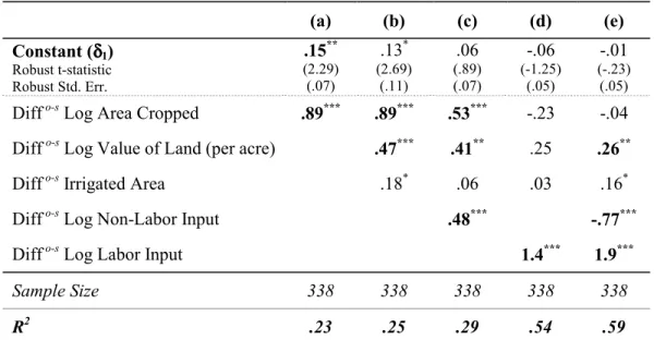
By comparing coefficients in Tables 3 and 5 one observes that correcting for the ability bias reduces the estimates forδ1. The results are consistent with those from section 4. Controlling for observable variables, there is no productivity gap between owned and sharecropped plots of the same household.
5.2
Mixed Owner & Fixed-Rent Tenant
Now, let us consider the subsample of households who owns and rent plots of the same product in the same year and season. Similarly to last section, the difference operator is defined to be such that:
Diffo-fZ = ˆ∆hZ =
P
i∈OhZi
Oh −
P
i∈FhZi
Fh ,
where Z is a generic variable; h indexes the observations; Oh (respectively, Fh) is the number of plots owned (respectively, rented) by h; and Oh and Fh as the
respective sets of those plots.
ˆ
∆hln(y) = (δ1−δ2) +
K
P
k=1
αk∆hˆ ln(xk) + ˆνh, (6)
where ˆνh =
P
i∈Ohui
Oh −
P
i∈Shui
Sh andV ar(ˆνh) =
³
1
Oh +
1
Fh
´
σ2 .
In Table 6, the constant term identifies the term (δ1−δ2). One cannot reject the hypothesis that owned and rented plots are equally productive. One must however be careful when interpreting those results, since the sample size is very small. (This implies a large standard deviation for the proposed estimator, so that the null hypothesis would hardly be rejected).
[INSERT TABLE 6]
Result 2. This section takes the ability bias into account. The results are con-sistent with those from section 4; suggesting that plots cropped under the three tenancy contracts are equally productive.
6
Complementarity vs. Imperfect Monitoring
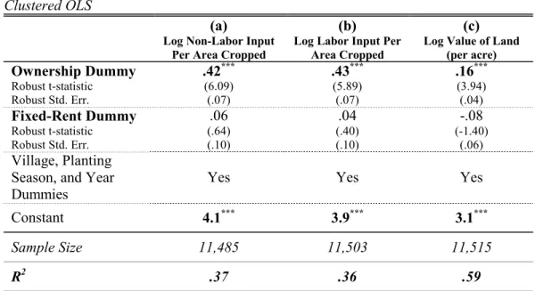
For all villages studied, share contracts are such that the tenant alone bears the cost of some inputs. This creates a distortion in the intensive margin (i.e., one bears the entire marginal cost and receives only a fraction of the marginal revenue), which would induce non-monitored sharecroppers to use less than the optimal level of non-labor and labor inputs. Sharecroppers indeed use less of those inputs per area cropped than owners, as shown by regressions (a) and (b) in Table 7. However, this may not be related to incentive problems, since fixed-rent tenants also use less inputs per area cropped than owners, and about as much as sharecroppers (see those same regressions). Moreover, sharecropping and fi xed-rent contracts are both associated with lower-quality lands −see regression (c) in Table 7. Therefore, complementarity among factors would explain why both types of tenants use less of those inputs.
[INSERT TABLE 7]
farmers’ optimal decisions and test if a standard degree of complementarity would be able to justify sharecroppers’ choices of inputs.
Efficient Input Level
The farmer’s ability and the quality of land are fixed factors. Also, the size of the farm is a decision made in the extensive margin (at the time of buying or renting the farm). Therefore, in each season, farmers choose the amount of labor and non-labor inputs. Since output and factors are measured in monetary units, the profit maximization problem faced by owners and fixed-rent tenants is:
maxxi3,xi4E{yi−xi1−xi2−c},
where yi =Ai K
Q
k=1
xαk
ik exp (εi), xi1 and xi2 are the value of non-labor and labor in-puts, andcstands for the rent (in the case offixed-rent tenants) or the opportunity cost of the farm (in the case of owners).
The necessary and sufficient first-order conditions are:
E
(
αjAix
αj−1
ij
Q
k6=j xαk
ik exp (εi)
)
= 1, j ∈{1,2}.
Alternatively, the above conditions can be rewritten as:
E
½
αj yi xij
¾
= 1, j ∈{1,2}. (7)
Non-Monitored Choices of Sharecroppers
In many villages, the landlord also shares the cost of some inputs, in which case there is no marginal distortion to be studied. However, when sharecroppers bear alone the cost of outputs, and if there is no informal agreement regarding the amount of inputs to be used, sharecroppers would maximize:
maxxi3,xi4E{siyi−xi1−xi2},
where yi = Ai
4
Q
k=1
xαk
ik exp (εi) and si is the fraction of output received by the
The necessary and sufficient conditions for the maximum are:
E
½
siαj yi xij
¾
= 1, j ∈{1,2}. (8)
Since 0< si <1 (by definition of sharecropping), the existence of monitoring problems would imply a higher expected productivity,E
n
αjxyiji
o
, in sharecropped plots.
6.1
Econometric Test
Whenever complementarity explains tenants’ input choices, the expected marginal productivity,Enαjxyi
ij
o
, should be the same across the different contracts. On the other hand, if monitoring is indeed a problem, one should observe a larger expected marginal productivity in the sharecropped plots.
Notice that the coefficientαj may differ across households, years, seasons, and
cropping patterns. For that reason, I restrict the analysis to the subsample of mixed tenants. It is implicitly assumed that αj is the same for each household
cropping the same product in a certain year and season. Therefore, one can use the ratio yi
xij to test the existence of monitoring imperfections.
Let us model the output-input ratio as a constant associated with the contract form plus an error term and, then, test if these constants are the same across contracts. Thus:
yi
xij =c1d o i +c2d
f
i +c3dsi +ηi, (9)
where c1, c2, and c3 are constants; doi, dfi, and dsi are the dummy variables for the tree contract forms (ownership, fixed rent, and sharecropping); and ηi is a error
term with zero mean and constant variance.
Remark 2. Under the null hypothesis that there is no monitoring problems, one must have c1 = c2 = c3. The alternative hypothesis is c1 = c2 < c3 (i.e., if
sharecroppers were not monitored, their expected marginal productivity would be higher).
Mixed Owner & Sharecropper
∆h yi
xij = (c1−c3) +∆hηi,
where var(∆hηi) =
³
1
Oh +
1
Sh
´
var(ηi).
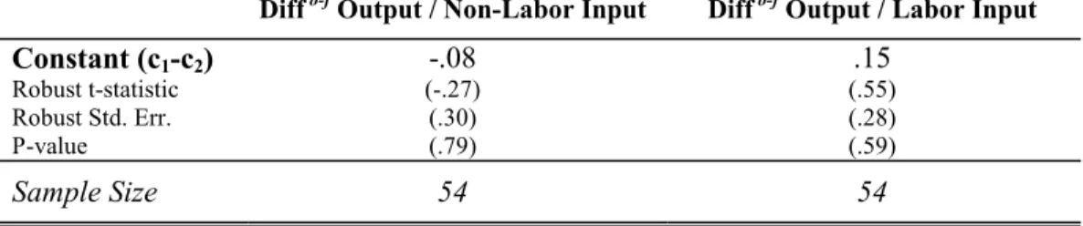
Table 8 presents the GLS estimations. The estimates for (c1 −c3) are non-significant, so that one cannot reject the hypothesis of perfect monitoring (i.e., the marginal productivity of non-labor and labor inputs are equal in owned and sharecropped plots of the same household).
[INSERT TABLES 8]
Mixed Owner & Fixed-Rent Tenant
Let us use now the subsample of mixed owner & fixed-rent tenant to identify the term(c1−c2). As in section 5.2, apply the operator ∆hˆ on (9), so that:
ˆ ∆h yi
xij = (c1−c2) + ˆ∆hηi,
where var(∆hηi) =
³
1
Oh +
1
Fh
´
var(ηi).
Table 9 shows that one cannot reject that the marginal productivity of non-labor and non-labor inputs are equal in owned and rented plots of the same household (i.e., c1 =c2).
[INSERT TABLES 9]
Result 3. No evidence of monitoring problems is found in the data set. The type of complementarity inherent in the Cobb-Douglas production function is able to justify sharecroppers’ input choices.
7
Sensitivity Analysis
This paperfinds no missing incentives associated with share contracts, and this result drastically differs from those in the current literature. As stated before, this paper is closely related to the one by Shaban (1987). We assess similar questions, with a similar data set, and obtain opposite conclusions. It is natural then to have some considerations about this.
(while Shaban uses a linear regression model for the output per area cropped). Second, I argue that non-labor and labor inputs must be taken into account, since complementarity implies that those choices are non-linearly affected by the quality of land (which is not randomly assigned to each contract form). Third, by using the benefit of addressing the same problem more than one decade later, I am able to access a larger number of years (from 1975 to 1984). Finally, my definition of mixed tenant is finer, which generates a more homogeneous sample.
Regarding this last difference, I compare plots of the same product cropped by the same household in a certain year and season, while Shaban does not control for the cropping pattern. This section is intended to show that the results are not sensitive to the definition of mixed tenants.
7.1
Mixed* Tenants
Let us use an asterisk to represent another possible way to aggregate the data. Mixed* tenants are those cropping multiple plots under different contracts in the same year and season (without controlling for the cropping pattern). As before, the sample is divided in three categories: (i) mixed* owner & sharecropper; (ii) mixed* owner &fixed-rent tenant; and (iii) mixed*fixed-rent tenant & sharecropper. This new grouping criteria generates more observations in each of these subsamples, which allows us to analyze them all.
7.1.1 Mixed* Owner & Sharecropper
Table 10 presents some characteristics of the subsample of households cropping owned and shared plots in a certain year and season.
[INSERT TABLE 10]
As in section 5, let us estimate the difference regression model in order to identify the parameter δ1. Table 11 presents the GLS results. Mainly, when one does not control for the cropping pattern, one gets larger estimates for δ1 (which indicates that owners crop product with higher value). However, as before, these estimates are non-significant when observable inputs are used as covariates.
Village Dummies
This new subsample is large enough to allow one to see the mean effect of the share contract across the different villages (notice however, from Table 10, that the number of observations is very small for some villages). In order to do that, let us replace the constant term with village dummies (see Table 12).
[INSERT TABLE 12]
For the villages of Aurapalle (A), Dokur (B), Shirapur (C), Boriya (G), and Ramputa, the productivity difference between owned and sharecropped lands is not statistically significant even without controlling for the quality of land and level of inputs. For the villages of Kalman (D) and Kanzara (E), the productivity gap is not significant when one controls for observable inputs. The results are not conclusive for the 26 observations from the village of Kinkheda (F).
7.1.2 Mixed* Owned & Fixed-Rent Tenant
As in section 5, one can identify the term (δ1−δ2) through the set of house-holds who own and rent plots in the same year and season. The composition of this subsample is described in Table 13 and the results are in Table 14. Controlling only for the area cropped, owned lands are more productive than those rented. Similarly to the previous subsection, this productivity gap is driven by observable variables. The results suggest that owned plots are apparently more productive than sharecropped lands due to the same reasons why they seem to be more pro-ductive than rented fields. Mainly, both types of tenants crop lower quality lands and, due to complementarity, they use less of the other inputs.
[INSERT TABLE 13]
[INSERT TABLE 14]
7.1.3 Mixed* Fixed-Rent Tenants & Sharecroppers
Finally, there is a very small subsample of households cropping lands under
fixed-rent and share contracts (in the same year and season). Let us now define:
Difff-s Z = ¯∆hZ =
P
i∈F
hZi
Fh −
P
i∈O
hZi
so that:
¯
∆hln(y) = δ2+
K
P
k=1
αk∆h¯ ln(xk) + ¯νh, (10)
where ¯νh =
P
i∈F
hui
Fh −
P
i∈S
hui
Sh andV ar(¯νh) =
³
1
Fh +
1
Sh
´
σ2 .
Table 15 describes the sample. The regressions in Table 16 show that there is no productive difference between rented and sharecropped plots cultivated by those mixed* tenants.
[INSERT TABLE 15]
[INSERT TABLE 16]
8
Conclusion
In this paper I test the existence of missing incentives in one of the classical examples of moral hazard: the landlord-tenant relationship.
First, I test how expected output of farms is affected by the tenancy contract. Sharecroppers are less productive than owners, but as productive as fixed-rent tenants (which contradicts the moral hazard predictions). Also, I show that the productivity gap between owners and both types of tenants is driven by sample-selection issues and observable variables. An endogenous sample-selection rule matches tenancy contracts with less-skilled farmers and lower-quality lands. Due to com-plementarity, such a matching also affects tenants’ choices of labor and non-labor inputs. I use a subsample of households cropping the same product under different contract forms in the same year and season, to account for selection bias and show that the contract form has no effect on the expected output.
References
[1] Ackerberg, Daniel A. and Botticini, Maristella. “Endogenous Match-ing and the Empirical Determinants of Contract Form.” Journal of Political Economy, 2001, forthcoming.
[2] Bandiera, Oriana. “On the Structure of Tenancy Contracts: Theory and Evidence from 19th Century Rural Sicily.” Mimeo, London School of Eco-nomics, 1999.
[3] Banerjee, Abhijit, Gertler, Paul, and Ghatak, Maitreesh. “Empow-erment and Efficiency: Tenancy Reform in West Bengal.” Journal of Political Economy, Forthcoming, 2001.
[4] Bhattacharyya, Sugato and Lafontaine, Francine.“Double-Sided Moral Hazard and the Nature of Share Contracts.” Rand Journal of Economics,
Winter 1995, 26 (4), 761-781.
[5] Binswanger, Hans P. and Jodha, N.S. “Manual of Instructions for Eco-nomic Investigators in ICRISAT’s Village Level Studies.” Hyderabad: Inter-national Crops Research Institute for Semi-Arid Tropics, 1978.
[6] Bisin, Alberto and Guaitoli, Danilo. “Moral Hazard and Non-Exclusive Contracts.” Mimeo, New York University, 2000.
[7] Braido, Luís H.B.“General Equilibrium with Endogenous Financial Design and Moral Hazard.” Mimeo, University of Chicago, 2001.
[8] Cardon, James and Hendel, Igal. “Asymmetric Information in Health Insurance: Evidence from NMES.” Rand Journal of Economics, 2001, forth-coming.
[9] Cheung, Steven N.S. “Sharecropping.” In “Famous Fables of Economics: Myths of Market Failures,” edited by Daniel F. Spulber, Blackwell Publishers Ltd, Oxford, U.K., 2002.
[11] Chiappori, Pierre-André and Salanié, Bernard.“Testing for Asymmet-ric Information in Insurance Markets.”Journal of Political Economy, Febru-ary 2000, 108 (1), pp. 56-78.
[12] Dionne, Georges and Doherty, Neil A.“Adverse Selection, Commitment, and Renegotiation: Extensions to and Evidence from Insurance Markets.”
Journal of Political Economy, April 1994, 102 (2), 209-235.
[13] Dionne, Georges and Vanasse, Charles. “Automobile Insurance Ratemaking in the Presence of Asymmetrical Information.”Journal of Applied Econometrics, April-June 1992, 7 (2), 149-165.
[14] Jodha, N.S., Asokan, M. and Ryan, J.C. “Village Study Methodology and Resource Endowment of the Selected Villages in ICRISAT’s Village Level Studies.” Economics Program Occasional Paper no. 16. Hyderabad: Interna-tional Crops Research Institute for Semi-Arid Tropics, 1977.
[15] Johnson, D. Gale. “Resource Allocation under Share Contracts.” Journal of Political Economy, April 1950, 58 (2), 111-123.
[16] Heckman, James J.“The Common Structure of Statistical Models of Trun-cation, Sample Selection and Limited Dependent Variables and a Simple Es-timator for Such Models.”The Annals of Economic and Social Measurement, Fall 1976, 5 (4), pp. 475-492.
[17] Heckman, James J. “Dummy Endogenous Variables in a Simultaneous Equation System.”Econometrica, July 1978, 46 (6), pp. 931-961.
[18] Heckman, James J. “Sample Selection Bias as a Specification Error.”
Econometrica, January 1979, 47 (1), pp. 153-162.
[19] Heckman, James J. and Robb, Richard Jr. “Alternative Methods for Evaluating the Impact of Interventions: An Overview.”Journal of Economet-rics, October-November 1985, 30 (1-2), pp. 239-267.
[20] Hendel, Igal and Lizzeri, Alessandro. “Optimal Dynamic Contracts: Ev-idence from Life Insurance.” Mimeo, Princeton University, 2001.
[22] Laffont, Jean-Jacques and Matoussi, Mohamed S.“Moral Hazard, Fi-nancial Constraints and Sharecropping in El Oulja.” Review of Economic Studies, July 1995, 62 (3), 381-399.
[23] Pandey, Priyanka. “Effects of Technology on Incentive Design of Share Contracts.” Mimeo, Pennsylvania State University, 2001.
[24] Prescott, Edward C. and Townsend, Robert M. “Pareto Optima and Competitive Equilibria with Adverse Selection and Moral Hazard.” Econo-metrica, January 1984, 52 (1), pp. 21-46.
[25] Puelz, Robert and Snow, Arthur.“Evidence on Adverse Selection: Equi-librium Signaling and Cross-Subsidization in the Insurance Market.”Journal of Political Economy, April 1994, 102 (2), pp. 236-257.
[26] Richaudeau, Didier. “Automobile Insurance Contracts and Risk of Acci-dent: An Empirical Test Using French Individual Data”,The Geneva Papers on Risk and Insurance Theory,June 1999, 24 (5), pp. 97-114.
[27] Shaban, Radwan A. “Testing between Competing Models of Sharecrop-ping.” Journal of Political Economy, October 1987, 95 (5), pp. 893-920.
TABLE 1. Data Description
Variable Description
Output Value of main output and byproducts (in Rupees, R$)
Ownership Dummy 1 if plot is owned (82.6%); 0 otherwise
Fixed-Rent Dummy 1 if plot is rented on a fix-rent basis (2%); 0 otherwise
Area Cropped Area of the plot actually cultivated (in acres)
Value of Land (per acre) Per acre estimated value of the plot, in 100R$
Irrigated Area Total irrigated area in the plot
Non-Labor Input
Value of seeds, fertilizers, pesticides, organic and inorganic manures, plus rental value of owned and hired bullock, and other machineries (in R$)
Labor Input Value of family and hired labor according to the village wages for males, females, and children (in R$)
Planting Season Dummies
35.2% planted from June to October; 59.2% from November to February; 5.3% from March to May; .2% perennial crops; .1% missing data
Village Dummies
14% Aurepalle; 5.2% Dokur; 21.1 Shirapur; 15.9% Kalman; 14% Kanzara; 5.4% Kinkheda; 9.1% Boriya; 15.3% Rampura
Year Dummies
1975 (11%); 1976 (11.2%); 1977 (10.8%); 1978 (9.5%); 1979 (9.2%); 1980 (9.6%); 1981 (10.5%); 1982 (9.7%); 1983 (9.3%); 1984 (9.2%)
Cropping Pattern Qualitative variable (with 1,031 different codes) describing all products cropped in a certain plot
Note: Data from the International Crops Research Institute for Semi-Arid Tropics (ICRISAT).
TABLE 2. Summary Statistics (Entire Sample)
Variable Mean Min Max St. Dev. Sample
Size
Output 901.3 0 22,768.8 1,338.6 11,517 Area Cropped 1.8 0 25 2.0 11,517
TABLE 3. Regression Model (Entire Sample)
Clustered OLS
Dependent Variable: Log Output
(a) (b) (c) (d) (e)
Ownership Dummy (δδδδ1)
Robust t-statistic Robust Std. Err.
.31***
(4.85) (.06)
.17***
(3.33) (.05)
.06
(1.45) (.04)
-.01 (-.46)
(.03)
-.01 (-.53)
(.03)
Fixed-Rent Dummy (δδδδ2)
Robust t-statistic Robust Std. Err.
-.05
(-.39) (.14)
-.02
(-.15) (.14)
-.07
(-.62) (.11)
-.07
(-.78) (.08)
-.07 (-.81)
(.08)
Log Area Cropped .68*** .68*** .30*** .05*** .05**
Log Value of Land (per acre) .56*** .32*** .19*** .18***
Irrigated Area .50*** .11*** .09*** .07***
Log Non-Labor Input .66*** .07***
Log Labor Input 1.0*** .96***
Village, Planting Season, and
Year Dummies Yes Yes Yes Yes Yes
Constant 6.9*** 6.3*** 1.7*** 1.2*** .65**
Sample Size 10,704 10,701 10,687 10,701 10,687
R2 .41 .51 .65 .76 .76
TABLE 4. Sample Characteristics (Mixed Tenants)
Number of Households Number of Plots
Mixed Owner & Sharecropper 338 609 owned; 585 sharecropped
Mixed Owner & Fixed-Rent Tenant 54 84 owned; 59 rented
Mixed Fixed-Rent Tenant &
Sharecropper 8 8 rented; 10 sharecropped
TABLE 5. Difference Regression (Mixed Owner & Sharecropper)
Clustered GLS
Independent Variable: Diff o-s Log Output
(a) (b) (c) (d) (e)
Constant (δδδδ1)
Robust t-statistic Robust Std. Err.
.15**
(2.29) (.07)
.13*
(2.69) (.11)
.06
(.89) (.07)
-.06
(-1.25) (.05)
-.01
(-.23) (.05)
Diff o-s Log Area Cropped .89*** .89*** .53*** -.23 -.04
Diff o-s Log Value of Land (per acre) .47*** .41** .25 .26**
Diff o-s Irrigated Area .18* .06 .03 .16*
Diff o-s Log Non-Labor Input .48*** -.77***
Diff o-s Log Labor Input 1.4*** 1.9***
Sample Size 338 338 338 338 338
R2 .23 .25 .29 .54 .59
TABLE 6. Difference Regression (Mixed Owner & Fixed-Rent Tenant)
Clustered GLS
Independent Variable: Diff o-f Log Output
(a) (b) (c) (d) (e)
Constant (δδδδ1 - δδδδ2)
Robust t-statistic Robust Std. Err.
.16
(.74) (.22)
.12
(.41) (.11)
-.07
(-.22) (.07)
.11
(.68) (.16)
.19
(1.12) (.17)
Diff o-f Log Area Cropped 1.2*** 1.1** .06 -.59* -.34
Diff o-f Log Value of Land (per acre) .37 .27 -.26 -.30
Diff o-f Irrigated Area .04 -.09 -.09 -.04
Diff o-f Log Non-Labor Input 1.2** -.54
Diff o-f Log Labor Input 2.4*** 2.7***
Sample Size 54 54 54 54 54
R2 .16 .16 .28 .70 .72
TABLE 7. Productive Inputs (Entire Sample)
Clustered OLS
(a) (b) (c)
Log Non-Labor Input Per Area Cropped
Log Labor Input Per Area Cropped
Log Value of Land (per acre)
Ownership Dummy
Robust t-statistic Robust Std. Err.
.42***
(6.09) (.07)
.43***
(5.89) (.07)
.16***
(3.94) (.04)
Fixed-Rent Dummy
Robust t-statistic Robust Std. Err.
.06
(.64) (.10)
.04
(.40) (.10)
-.08
(-1.40) (.06)
Village, Planting Season, and Year Dummies
Yes Yes Yes
Constant 4.1*** 3.9*** 3.1***
Sample Size 11,485 11,503 11,515
R2 .37 .36 .59
TABLE 8. Marginal Productivity (Mixed Owner & Sharecropper)
Clustered GLS
Diff o-s Output / Non-Labor Input Diff o-s Output / Labor Input
Constant (c1-c3)
Robust t-statistic Robust Std. Err. P-value
-.08
(-.44) (.18) (.66)
.02
(.19) (.11) (.85)
Sample Size 338 338
Note: Number of clusters equals 82.
TABLE 9. Marginal Productivity (Mixed Owner & Fixed-Rent Tenant)
Clustered GLS
Diff o-f Output / Non-Labor Input Diff o-f Output / Labor Input
Constant (c1-c2)
Robust t-statistic Robust Std. Err. P-value
-.08
(-.27) (.30) (.79)
.15
(.55) (.28) (.59)
Sample Size 54 54
TABLE 10. Sample Characteristics (Mixed* Owner & Sharecropper)
Number of Households
Number of Owned Plots
Number of Sharecropped Plots
Aurapalle (A) 4 10 7
Dokur (B) 33 70 61
Shirapur (C) 123 562 433
Kalman (D) 84 417 340
Kanzara (E) 54 239 145
Kinkheda (F) 26 65 51
Boriya (G) 78 217 206
Rampura (H) 26 273 230
TOTAL 454 1,853 1,473
TABLE 11. Difference Regression (Mixed* Owner & Sharecropper)
Clustered GLS
Independent Variable: Diff o-s Log Output
(a) (b) (c) (d) (e)
Constant (δδδδ1)
Robust t-statistic Robust Std. Err.
.41***
(3.69) (.11)
.29***
(2.69) (.11)
.03
(.34) (.09)
-.04
(-.60) (.06)
-.02
(-.30) (.07)
Diff o-s Log Area Cropped .56*** .66*** .13 -.12 -.10
Diff o-s Log Value of Land (per acre) .71*** .36** .21** .23**
Diff o-s Irrigated Area .60*** .08 -.03 .002
Diff o-s Log Non-Labor Input 1.0*** -.18
Diff o-s Log Labor Input 1.4*** 1.6***
Sample Size 454 454 454 454 454
R2 .10 .18 .39 .61 .61
TABLE 12. Village Effects (Mixed* Owner & Sharecropper)
Clustered GLS
Independent Variable: Diff o-s Log Output
(a) (b) (c) (d) (e)
Aurapalle (A) Robust t-statistic Robust Std. Err.
.62 (1.08) (.58) .70 (1.35) (.52) .21 (.45) (.47) -.06 (-.13) (.45) -.04 (-.08) (.46) Dokur (B) Robust t-statistic Robust Std. Err.
.03 (.13) (.25) -.09 (-.32) (.29) -.12 (-.80) (.16) -.20** (-2.23) (.09) -.20 (-1.76) (.11) Shirapur (C) Robust t-statistic Robust Std. Err.
.34 (1.28) (.26) .25 (1.18) (.21) .16 (.88) (.18) -.04 (-.32) (.12) -.05 (-.43) (.12) Kalman (D) Robust t-statistic Robust Std. Err.
.76*** (3.14) (.24) .63*** (2.66) (.24) .18 (.96) (.19) -.03 (-.34) (.10) -.01 (-.11) (.10) Kanzara (E) Robust t-statistic Robust Std. Err.
.96*** (2.96) (.33) .69** (2.04) (.34) .31 (1.21) (.26) .30 (1.44) (.21) .34 (1.52) (.23) Kinkheda (F) Robust t-statistic Robust Std. Err.
.56** (2.39) (.23) .51** (2.20) (.23) .12 (.84) (.14) .23* (1.85) (.12) .28* (1.92) (.14) Boriya (G) Robust t-statistic Robust Std. Err.
-.07 (-.42) (.18) -.08 (-.45) (.17) -.22 (-1.31) (.17) -.20* (-1.79) (.11) -.19* (-1.67) (.11) Rampura (H) Robust t-statistic Robust Std. Err.
.33 (.87) (.38) .15 (.49) (.30) -.19 (-1.06) (.18) -.10 (-.53) (.19) -.06 (-.26) (.22)
Diff o-s Log Area Cropped .57*** .66*** .17 -.12 -.10
Diff o-s Log Value of Land (per acre) .67*** .34** .20** .22**
Diff o-s Irrigated Area .58*** .08 -.05 -.01
Diff o-s Log Non-Labor Input .98*** -.21
Diff o-s Log Labor Input 1.4*** 1.6***
Sample Size 454 454 454 454 454
Adjusted R2 .14 .21 .40 .62 .62
TABLE 13. Sample Characteristics (Mixed* Owner & Fixed-Rent Tenant)
Number of Households
Number of Owned Plots
Number of Rented Plots
Aurapalle (A) 26 75 31
Dokur (B) 4 24 5
Shirapur (C) 2 8 3
Kalman (D) 2 12 2
Kanzara (E) 26 168 38
Kinkheda (F) 1 3 1
Boriya (G) 35 97 64
Rampura (H) 35 141 48
TOTAL 124 528 192
TABLE 14. Difference Regression (Mixed* Owner & Fixed-Rent Tenant)
Clustered GLS
Independent Variable: Diff o-f Log Output
(a) (b) (c) (d) (e)
Constant (δδδδ2 - δδδδ1)
Robust t-statistic Robust Std. Err.
.42**
(2.46) (.17)
.30**
(1.74) (.18)
.17
(1.10) (.15)
.10
(.75) (.13)
.13
(1.01) (.13)
Diff o-f Log Area Cropped 1.0*** .89*** .31 -.41 -.35
Diff o-f Log Value of Land (per acre) .59** .38 .04 .05
Diff o-f Irrigated Area .47*** -.06 -.23** -.08
Diff o-f Log Non-Labor Input .94*** -.49**
Diff o-f Log Labor Input 2.0*** 2.4***
Sample Size 124 124 124 124 124
R2 .11 .17 .29 .62 .64
TABLE 15. Sample Characteristics (Mixed* Fixed-Rent Tenant & Sharecropper)
Number of Households
Number of Rented Plots
Number of Sharecropped Plots
Aurapalle (A) 0 0 0
Dokur (B) 2 3 2
Shirapur (C) 0 0 0
Kalman (D) 0 0 0
Kanzara (E) 12 20 32
Kinkheda (F) 1 1 1
Boriya (G) 6 8 13
Rampura (H) 11 21 37
TOTAL 32 53 85
TABLE 16. Difference Regression (Mixed* Fixed-Rent Tenant & Sharecropper)
Clustered OLS
Independent Variable: Diff f-s Log Output
(a) (b) (c) (d) (e)
Constant (δδδδ2)
Robust t-statistic Robust Std. Err.
.05
(.16) (.30)
-.15
(-.47) (.32)
-.20
(-.67) (.30)
.05
(.18) (.26)
.16
(.78) (.21)
Diff f-s Log Area Cropped .32 .33 -.01 -.46 -.53
Diff f-s Log Value of Land (per acre) .88* .62 -.08 -.26
Diff f-s Irrigated Area .64** -.18 -.04 .27
Diff f-s Log Non-Labor Input .96** -.68
Diff f-s Log Labor Input 1.6*** 2.2***
Sample Size 32 32 32 32 32
R2 .02 .14 .32 55 .58