Calculations of the integral invariant coordinates I and L* in the magnetosphere and mapping of the regions where I is conserved, using a particle tracer (ptr3D v2.0), LANL*, SPENVIS, and IRBEM

(1)

www.geosci-model-dev.net/8/2967/2015/ doi:10.5194/gmd-8-2967-2015

Calculations of the integral invariant coordinates

_I

and

_L

∗

_{in the}

magnetosphere and mapping of the regions where

_I

is conserved,

**using a particle tracer (ptr3D v2.0), LANL*, SPENVIS, and IRBEM**

K. Konstantinidis1,aand T. Sarris1

1_{Department of Electrical and Computer Engineering, Democritus University of Thrace, Xanthi, Greece} a_{now at: Department of Aerospace Engineering, Bundeswehr University, Munich, Germany}

Correspondence to:T. Sarris (tsarris@ee.duth.gr)

Received: 14 July 2014 – Published in Geosci. Model Dev. Discuss.: 26 September 2014 Revised: 19 January 2015 – Accepted: 1 September 2015 – Published: 28 September 2015

Abstract.The integral invariant coordinateIand Roederer’s

LorL∗are proxies for the second and third adiabatic invari-ants, respectively, that characterize charged particle motion in a magnetic field. Their usefulness lies in the fact that they are expressed in more instructive ways than their counter-parts:I is equivalent to the path length of the particle motion between two mirror points, whereasL∗, although dimension-less, is equivalent to the distance from the center of the Earth to the equatorial point of a given field line, in units of Earth radii, in the simplified case of a dipole magnetic field. How-ever, care should be taken when calculating the above invari-ants, as the assumption of their conservation is not valid ev-erywhere in the Earth’s magnetosphere. This is not clearly stated in state-of-the-art models that are widely used for the calculation of these invariants. The purpose of this work is thus to investigate where in the near-Earth magnetosphere we can safely calculateIandL∗with tools with widespread use in the field of space physics, for various magnetospheric conditions and particle initial conditions.

More particularly, in this paper we compare the values of I andL∗ as calculated using LANL*, an artificial neu-ral network developed at the Los Alamos National Labora-tory, SPENVIS, a space environment online tool, IRBEM, a software library dedicated to radiation belt modeling, and ptr3D, a 3-D particle tracing code that was developed for this study. We then attempt to quantify the variations between the calculations ofI andL∗_{of those models. The deviation} be-tween the results given by the models depends on particle initial position, pitch angle and magnetospheric conditions. Using the ptr3D v2.0 particle tracer we map the areas in the

Earth’s magnetosphere whereI andL∗ can be assumed to be conserved by monitoring the constancy ofI for energetic protons propagating forwards and backwards in time. These areas are found to be centered on the noon area, and their size also depends on particle initial position, pitch angle and magnetospheric conditions.

1 Introduction

The motion of charged particles in the geomagnetic field is complicated, even if one approximates that field with only its dipole component. It is helpful to break down the total motion of the particle into three individual components: gy-ration around a guiding magnetic field line, bounce along the magnetic field line between magnetic mirror points, and gra-dient and curvature drift across the magnetic field line in an azimuthal direction around the Earth. Because these compo-nents evolve over very different time scales, they are nearly independent of each other and can thus be summed linearly to obtain the total motion (Prölss, 2004). For time variations of the magnetic field that are slow compared to the correspond-ing timescale of each type of motion, an adiabatic invariant is defined.

(2)

where the integral is between two mirror points,B(s)is the magnetic field intensity and ds the line element along the field line, andBmis the magnetic field intensity at the mir-ror points.I is expressed in distance units (km or RE) and depends on the length of the particle trajectory along a field line between the two mirror points. In place of the third adi-abatic invariant it is convenient to use L∗ or Roederer’sL

(Roederer, 1970).L∗is defined as

L∗= −2π k0

8RE

, (2)

wherek0is the Earth’s dipole moment,REis the radius of the Earth (6370 km) and8is the third adiabatic invariant and is defined as

8= Z

S

Bds (3)

integrated along the trajectory of the particle for the entire drift shell.

L∗physically approximates the distance from the center of the Earth to the equatorial point of a given field line (inRE) if we assume a dipolar magnetic field for the Earth.L∗_{is also} an invariant, since it is inversely proportional to8(Roederer, 1970).

A practical way to calculate8is to find the intersection

Cof a series of drift-shell field lines with the Earth’s surface and to numerically compute8over the cap delineated byC, using the following equation:

8≃ −k0

RE 2π Z

0

cos2[λe(φ)]dφ, (4)

whereλe(φ)is the dipole latitude of the intersectionC at a given longitudeφ(Roederer, 1970).

2 Programs used 2.1 LANL*

In general, calculation of L∗ is very computationally ex-pensive because it involves an integral that is both two-dimensional and global. LANL* aims to address this issue

first layer provides 19 nodes, one for each input parameter for the TS05 model plus additional nodes to help specify the drift shell especially for low Earth orbit. The hidden layer in the neural network contains 20 neurons that are connected to each input node and one output node to produceL∗_{. The} ANN was trained using the latest version of the IRBEM-lib IRBEM-library in SpacePy, a Python-based tool IRBEM-library for space science, to generate the input–output database, using a con-strained truncated Newton algorithm to train an ANN on the input–target data. A second neural network within LANL* V2.0 called LANLmax was created to describe the last closed drift shell (maximum possible value forL∗) under the spec-ified solar wind conditions (Koller and Zaharia, 2011; Yu et al., 2012).

LANL* V2.0 can be downloaded at http://www.lanlstar. lanl.gov/download.shtml.

2.2 IRBEM-lib

IRBEM-lib (formerly known as ONERA-DESP-LIB) is a freely distributed library of source codes dedicated to ra-diation belt modeling put together by the Office National d’Etudes Aérospatiales (ONERA-DESP). The library allows the computation of magnetic coordinates and fields for any location in the Earth’s environment for various magnetic field models. It is primarily written in Fortran with access to a shared library from IDL or Matlab (Bourdarie and O’Brien, 2009). IRBEM-lib calculatesI by tracing the magnetic field line that crosses a given point, calculating the integrand of Eq. (1) along all line elements of the field line1. The third invariant8is evaluated in IRBEM-lib using the numerical method described by Roederer as given in the introduction, where the magnetic drift shell is defined as a set of magnetic field line segments where all the segments are characterized by the same shell parameter and the same mirror-point mag-netic field intensity. Roederer’s shell parameter L∗ is then deduced directly from the value of the third invariant using Eq. (2)2_.

1_{As seen in the IRBEM source code, e.g., irbem/trunk/source/}

trace_drift_shell.f.

2_{As found in the IRBEM source code, also in irbem/trunk/}

(3)

Figure 1.Calculations ofIas a function of initial distance (inRE)

at 12:00 MLT, for pitch angles of 15, 30, 45 and 60◦and quiet solar wind conditions.

The latest version of IRBEM-lib can be found at http:// sourceforge.net/projects/irbem/.

2.3 SPENVIS

The European Space Agency (ESA) Space Environment Information System (SPENVIS) provides standardized ac-cess to models of the hazardous space environment through a World Wide Web interface (Heynderickx et al., 2004). SPENVIS includes magnetic field models implemented by means of the UNILIB library for magnetic coordinate eval-uation, magnetic field line tracing and drift shell tracing. Among these models are TS05 external and IGRF internal models. In UNILIB, the integral invariantI is evaluated us-ing a Runge–Kutta integration technique to evaluate Eq. (1) for a temporary magnetic field line, also traced in UNILIB (Schmitz et al., 2000). The third invariant8is evaluated in UNILIB using Roederer’s numerical method as for the case of IRBEM-lib3.

The SPENVIS web interface can be accessed at http: //www.SPENVIS.oma.be/. The UNILIB library can be found at http://www.magnet.oma.be/unilib/.

2.4 ptr3D v2.0

The calculations of I andL∗ were also performed using a 3-D particle tracing code that was developed for this study (ptr3D v2.0). This code traces the full 3-D Lorentz motion of single charged particles by integrating the relativistic Lorentz equation in the same geomagnetic field model that was used in the above simulations, the TS05, for direct comparison be-tween all the models considered here. In the particle tracing model the integration is performed by means of Hamming’s modified predictor–corrector method in conjunction with a fourth-order Runge–Kutta method for initialization (Ralston

3_{Reference: UNILIB source code.}

at 00:00 MLT, for pitch angles of 15, 30, 45 and 60◦and quiet solar wind conditions.

and Wilf, 1977; Ralston, 1962). For the calculations of the magnetic field, the GEOPACK-2008 implementation of the TS05 magnetic field model was used (Kuznetsova, 2006).

ptr3D v2.0 calculatesI by directly evaluating Eq. (1) for each step of the simulation. The third invariant8is calcu-lated following the method described by Roederer (1970). Roederer’s shell parameterL∗is then deduced directly from the value of the third invariant using Eq. (2).

3 Calculations ofI

The integral invariantI was calculated for various geocen-tric distances (inRE, GSM) using IRBEM and SPENVIS, for particles starting at magnetic local noon and magnetic local midnight, during quiet and disturbed magnetospheric conditions. Four initial pitch angles (15, 30, 45 and 60◦) and five initial distances (4–8REin steps of 1RE) were used. Us-ing the ptr3D particle tracer,I was calculated for 3 particle energies (500 keV, 1 MeV and 4 MeV), 5 initial distances (4– 8REin steps of 1RE) and 12 initial particle gyrophases, also during quiet and disturbed magnetospheric conditions (in a static magnetic field), and the finalI was estimated as the median of the results for all gyrophases.

In Figs. 1 to 3 the integral invariantI is shown as a func-tion of the distance of the starting point on the GSEx axis, in RE. Four families of curves are plotted, one for each initial pitch angle. The calculations in Figs. 1 and 2 were performed for quiet magnetospheric conditions (23 Febru-ary 2008, 17:55 UT was selected), for initial starting points at noon MLT and midnight MLT respectively, whereas the calculations in Fig. 3 were performed for disturbed magneto-spheric conditions (8 September 2002, 01:00 UT), for initial starting points at noon MLT.

(4)

at 12:00 MLT, for pitch angles of 15, 30, 45 and 60◦and disturbed solar wind conditions.

increases as one moves towards greater geocentric distances and also thatIis larger for greater pitch angles. Both of these cases can be explained if the connection betweenI and the bounce path length is considered: in the first case, the geo-centric distance of the particle increases, and the magnetic field lines become longer between two given mirror points. Therefore the particle’s path length increases accordingly. For the second case, particles with smaller equatorial pitch angles are mirrored further along a magnetic field line and therefore traverse greater distances along said field line than particles with greater equatorial pitch angles. A small devi-ation is observed in the results from ptr3D, which increased for increasing particle energy. This deviation is more pro-nounced for smaller pitch angles and for the 4 MeV case, whereas it is very small for the other two energy cases, and it becomes negligible for larger pitch angles.

In Fig. 2, where the calculations at midnight MLT are shown, the results from IRBEM and SPENVIS agree quite well for all cases. The results from ptr3D deviate from the results from IRBEM and SPENVIS in the following ways: there is a spread in the results that increases for increas-ing distances. The results for I deviate more from those of SPENVIS and IRBEM the greater the energy of the particle. This spread also becomes wider as the pitch angle decreases. In Fig. 3 a similar trend is observed, where for small pitch angles there is good agreement between SPENVIS and IRBEM and a deviation of the results from the 3-D tracer that is proportional to the particle energy. In this case though only the results for the 4 MeV particle deviate significantly from the rest. Furthermore, I appears to be larger as calcu-lated by ptr3D for higher particle energies, contrary to the figures above.

There is generally good agreement between the results from IRBEM and SPENVIS and those from ptr3D for 500 keV and 1 MeV particles, except for the case of 15◦pitch angle, where there is a small deviation at 5 and 6RE. Again

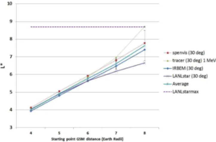
Figure 4.Calculations ofL∗as a function of initial distance (in

RE) at 00:00 MLT, for an initial pitch angle of 30◦ during quiet

solar wind conditions. Error bars represent the standard deviation between results from the various models.

it can be seen that the results for the 4 MeV particles deviate significantly and that this deviation is a function of distance and pitch angle, even though in this case we get a larger de-viation for larger pitch angles and the values forI are larger than those calculated with IRBEM and SPENVIS.

(5)

Figure 6. Calculations ofL∗ as a function of initial distance (in

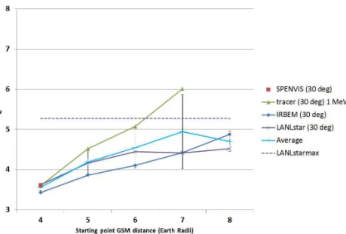
Figure 7. Calculations ofL∗ as a function of initial distance (in

RE) at 00:00 MLT, for an initial pitch angle of 30◦during disturbed

4 Calculations ofL∗

In the following,L∗was calculated using LANL*, IRBEM, SPENVIS and ptr3D for particles initiating their trajectory at 12:00 MLT on the XGSE axis, for five initial distances from 4 to 8REand for three initial pitch angles of 30, 60 and 90◦. The value ofL∗was also calculated for the last closed drift shell, calledL∗

max, using LANL* for the three pitch angles listed above. The results for the calculations during quiet and disturbed magnetospheric conditions are shown respectively in Figs. 4 to 9. These figures give the calculatedL∗_{as a} func-tion of distance inRE(in GSM) of the particle starting point on the magnetic equator and the point of calculation for all the other models used. L∗_maxcalculated through LANL* is also shown as a horizontal line.

Generally, for the quiet conditions case, the results from all the models tend to agree more at smaller distances (4–

6RE) and less further away (7–8RE). Also, the larger the initial pitch angle the greater the spread of the calculatedL∗. For example, the standard deviation becomes close to 2 for a distance of 8REand a pitch angle of 30◦.L∗maxis calculated to be around 9REfor all initial pitch angles.

(6)

Figure 10.I as a function of the particle’s azimuth angle for the case 1 MeV protons starting at GSM coordinates [8, 0, 0] (inRE) with

initial pitch angles of 30◦, and initial gyrophases of 0–330◦(30◦step). Particles propagating forwards in time are shown in blue, while those propagating backwards are shown in red.

Figure 11.The Lorenz trace of the forwards (blue) and backwards (red) propagating particle is plotted. The region whereIis constant according to Fig. 10 is shown in magenta. The contours of constant magnetic field strength are also plotted.

the results for each initial gyrophase. If more than half of the particles failed to complete a rotation around the Earth, no

L∗was calculated.

5 Mapping regions of constantI

Next, we demonstrate at which magnetic longitude the con-servation ofI is broken, for different particle starting condi-tions. We thus map the areas whereIand thereforeL∗cannot be safely calculated.

Using ptr3D, I was calculated for particles propagat-ing both forwards and backwards in time, durpropagat-ing the same two periods of quiet and disturbed solar wind conditions as above (23 February 2008, 17:55 UT and 8 September 2002, 01:00 UT respectively) starting at local noon, for 2 initial pitch angles (30 and 60◦), 5 initial distances (4–8RE) and for 12 initial particle gyrophases. For each pitch angle, the values ofI were plotted for each initial distance and initial gyrophase, both for forwards- and backwards-traced parti-cles, starting at local noon, as a function of the particle’s az-imuth angle. In the resulting plot, for both directions of prop-agation, a dashed vertical line marks the approximate point whereI stops being constant (see Figs. 10 and 11). Subse-quently, for each case of solar wind conditions and initial pitch angles, a map was created, depicting the areas whereI

(7)

Figure 12.Plots of the regions of constantI, for quiet and disturbed solar wind conditions, and 30 and 60◦initial equatorial pitch angles, for particle starting distances 4–8RE.

whereI ceases to be adiabatic. In these areas the general-purpose models and tools described above, such as IRBEM, LANL* and SPENVIS, cannot be safely used to calculate the values of the adiabatic invariantI and thereforeL∗.

5.1 Quiet conditions

In the case of the 30◦initial pitch angle,I remains constant throughout the path of the particle around the Earth for an initial particle distance of 4 and 5RE. For other initial dis-tances there appears to be a region in the nightside whereI

is no longer conserved. This region becomes larger with in-creasing distance. In the case of the 60◦initial pitch angle,I

remains constant throughout the path of the particles around the Earth for initial particle distances of 4–6RE. Similar to the case of particles with a 30◦initial pitch angle, there are regions whereI is not constant and these regions are larger

the longer the initial distance. Generally, the extent of these regions is smaller in the case of the 60◦ initial pitch angle particle.

5.2 Disturbed conditions

(8)

pitch angles, for both quiet and disturbed magnetospheric conditions and for particles initiating their motion both in the dayside and nightside.

The results for the calculations ofI in the dayside show that the models used are in good agreement for all geocen-tric distances of the particle starting positions, all pitch an-gles, and both for quiet and disturbed magnetospheric con-ditions. In the nightside and for quiet magnetospheric condi-tions, there is good agreement between models only for small geocentric distances of the particle starting positions, for all initial pitch angles. For larger distances, there is an increas-ing disagreement between these results, and differences are more accentuated for smaller pitch angles.

Generally, the same trends are observable for the calcula-tions of L∗ between the various models. For quiet magne-tospheric conditions the results from the models are in rela-tive agreement for smaller geocentric distances of the parti-cle starting positions and start to deviate with increasing dis-tances and initial pitch angles. For disturbed magnetospheric conditions this deviation is more accentuated.

Using ptr3D we mapped the areas in the Earth’s magneto-sphere whereI, and consequently alsoL∗, can be assumed to be conserved, for two initial pitch angles, and for both quiet and disturbed magnetospheric conditions. This too was per-formed by monitoring the constancy ofI for energetic pro-tons propagating forwards and backwards in time. Results for quiet magnetospheric conditions show that the regions where

I cannot be assumed to be conserved appear between a GSM distance of 5–7REin the nightside, centered at the midnight point depending on the pitch angle, and those areas expand on the nightside for larger distances. These areas are more extensive for larger particle pitch angles and appear to be symmetrical around the plane defined by the midnight–noon line and the Earth magnetic dipole axis. For disturbed mag-netospheric conditions, the areas whereI cannot be assumed to be conserved start to appear between a GSM distance of 3–5REon the nightside.

In the discussions of particle transport, energization and loss in the Earth’s radiation belts, a major question con-cerns the relative contribution between wave–particle inter-actions vs. radial diffusion, which is generally best discussed in terms of phase-space density, calculated at constant

adi-adiabatic in terms of their second and third invariants. The physical mechanism that leads to breaking of the in-variants in the regions illustrated does not involve temporal variations in the magnetic field of timescales shorter than the associated timescales of the second and third invariants, i.e., the bounce period and drift period, as the fields used in the simulations above are all static. Instead, the breaking of the invariants in the above is associated with deviations of the magnetic field from a dipole configuration: in the defini-tion of the invariants, in order for the second adiabatic in-variant to remain constant it is required that the magnetic field between two mirroring points does not change much in one bounce period as the particle’s guiding center drifts across field lines. Similarly, in order for the third adiabatic invariant to remain constant, it is required that the magnetic flux through the guiding center orbit of a particle around the Earth should remain constant. However during active geo-magnetic conditions the curvature of the field lines in the nightside of the Earth in combination with the large gyro-radii of large-energy particles leads to deviations from these conditions that need to be taken into account.

The present paper by no means aims to serve as a guideline of the adiabaticity of particles at all energies, pitch angles and geomagnetic conditions; instead, it aims to raise awareness and caution in using general-purpose models and tools, such as IRBEM, LANL* and SPENVIS, to calculate the values of the adiabatic invariants in regions and cases where they are not well defined.

Code availability

(9)

its next version (ptr3D V3.0) will be released as a general particle tracer code that can be used for any range of particle energies, times or regions.

Acknowledgements. This study was supported by NASA grants (THEMIS, NNX10AQ48G and NNX12AG37G) and NSF grant ATM 0842388. This research has also been co-financed by the European Union (European Social Fund – ESF) and Greek national funds through the Operational Program “Education and Lifelong Learning” of the National Strategic Reference Framework (NSRF) Research Funding Program: Thales. Investing in knowledge society through the European Social Fund.

Edited by: J. Koller

References

Bourdarie, S. and O’Brien, T. P.: International radiation belt en-vironment modelling library, COSPAR Panel on Radiation Belt Environment Modelling (PRBEM), 2009.

Heynderickx, D., Quaghebeur, B., Wera, J., Daly, E. J., and Evans, H. D. R.: New radiation environment and effects mod-els in the European Space Agency’s Space Environment In-formation System (SPENVIS), Space Weather, 2, S10S03, doi:10.1029/2004SW000073, 2004.

Koller, J. and Zaharia, S.: LANL*V2.0: global modeling and valida-tion, Geosci. Model Dev., 4, 669–675, doi:10.5194/gmd-4-669-2011, 2011.

Kuznetsova, M.: Tsyganenko geomagnetic field model and Geopack libraries, available at: http://ccmc.gsfc.nasa.gov/ models/ (last access: 23 September 2015), August 2006. Prölss, G.: Physics of the Earth’s Space Environment: An

Introduc-tion, Springer-Verlag, Berlin, Heidelberg, 2004.

Ralston, A.: Runge-Kutta methods with minimum error bounds, Math. Comput., 16, 431–437, 1962.

Ralston, A. and Wilf, H. S.: Mathematical methods for digital com-puters, Wiley, New York/London, 1977.

Roederer, J. G.: Dynamics of Geomagnetically Trapped Radiation, Springer-Verlag, Berlin, Heidelberg, 1970.

Schmitz, H., Orr A., and Lemaire, J.: Validation of the UNILIB Fortran library, Bulgarian-Belgian Cooperation Project, 362 p., 2000.

Calculations of the integral invariant coordinates <I>I</I> and <I>L</I>* in the magnetosphere and mapping of the regions where <I>I</I> is conserved, using a particle tracer (ptr3D v2.0), LANL*, SPENVIS, and IRBEM