HIKMAT ULLAH JAN
EFFICIENCY OF QTL MAPPING BASED ON LEAST SQUARES, MAXIMUM LIKELIHOOD, AND BAYESIAN APPROACHES UNDER HIGH MARKER
DENSITY
Thesis submitted to Federal University of Viçosa, in partial fulfillment of the requirements of the Genetics and Breeding Graduate Program, for the Degree of Doctor Scientiae.
VIÇOSA
ii
I dedicate this humble effort to my parents, especially to my late mother Robia Gula, teachers, and friends
iii
ACKNOWLEDGMENTS
All praises to Almighty Allah, The most Beneficent, the most Merciful, Who bestowed me with the potential and ability to complete my research work.
I am thankful to National Council for Scientific and Technological Development (CNPq), The World Academy of Sciences (TWAS) and United Nations Educational, Scientific and Cultural Organization (UNESCO) for financial support.
I owe my gratitude and feel it a privilege to pay my profound respect to my supervisor Prof. Dr. José Marcelo Soriano Viana, for his valuable suggestions and kind interest in this research work.
I am grateful to my teacher Prof. Dr. Aluízio Borém de Oliveira, Coordinator of the Graduate Program in Genetics and Breeding, for his support and valuable suggestion during the course of my degree program.
Heartiest thanks are due to my teacher Prof. Dr. Cosme Damião Cruz, for his constant help and sympathetic attitude towards the completion of the studies.
I wish to extend my sincere gratitude to Prof. Dr. Fabyano Fonseca e Silva, Prof. Dr. Vinícius Ribeiro Faria, Prof. Dr. Camila Ferreira Azevedo, and Dr. Antônio Carlos Baião de Oliveira, for their participation in thesis defense and valuable suggestions.
I also wish to extend my thanks to Prof. Dr. Moysés Nascimento and Prof. Dr. Rodrigo Oliveira de Lima, for participation in my Qualification exam.
I am thankful to Prof. Dr. Carlos S. Sediyama, Prof. Dr. Tuneo Sediyama, Prof. Dr. Ney S. Sakiyama, Prof. Dr. Leonardo L. Bhering, Prof. Dr. Felipe L. da Silva and Prof. Dr. Sérgio Y. Motoike, for their kind help and guidance during my studies.
I wish my thanks to Higher Education Department KPK Pakistan, for the grant of study leave.
Words cannot express my feelings of thanks and gratitude for my parents and family, seniors, colleagues, and friends since my graduation for their help.
In the end, I want to present my unbending thanks to all those hands who prayed for my betterment and serenity.
iv
BIOGRAPHY
v
SUMMARY
LIST OF TABLES vi
RESUMO vii
ABSTRACT viii
1. Introduction 1
2. Materials and Methods 4
2.1. Simulation 4
2.2. Genetic model 6
2.3. Methods of estimation 7
2.4.Hypothesis test and Bayesian inference 9
2.5.Statistical analysis 10
3. Results 11
3.1.Least squares and maximum likelihood approaches 11
3.2.Bayesian approach 12
3.3.Factors affecting the QTL mapping efficiency 14
4. Discussion 16
5. Acknowledgments 21
6. References 21
vi
LIST OF TABLES
Description Page
Table 1. Average number of QTLs† (Nqtl) and 95% confidence interval or highest probability density region width (CIw/HPDw) for the QTL position, from the least squares, maximum likelihood, and Bayesian approaches, regarding three traits, two heritabilities, and two sample sizes
25
Table 2. Average power of QTL detection† (%) and number of false QTLs in chromosomes with zero, one, and two to three true QTLs, from the least squares, maximum likelihood, and Bayesian approaches, regarding three traits, two heritabilities, and two sample sizes
26
Table 3. Average power of simultaneous detection of two and three
QTLs (%) from the least squares, maximum likelihood, and Bayesian approaches, regarding three traits, two heritabilities, and two sample sizes
27
Table 4. Average bias† (cM) in the estimated QTL position, from the least squares, maximum likelihood, and Bayesian approaches, regarding three traits, two heritabilities, and two sample sizes
28
Table 5. Average additive and dominance variances, and percentage
of the phenotypic variance explained by each QTL† from the least squares, maximum likelihood and Bayesian approaches, regarding three traits, two heritabilities, and two sample sizes
29
Table 6. Average number of QTLs (Nqtl), 95% confidence interval
or high probability density region width (CIw/HPDw), power of QTL detection (%), number of false QTLs in chromosomes with zero, one, and two to three true QTLs, power of simultaneous detection of two and three QTLs (%), bias (cM) in the estimated QTL position, and percentage of the phenotypic variance explained by each QTL, from the least squares and Bayesian approaches, regarding grain yield, two heritabilities, and two sample sizes
vii
RESUMO
JAN, Hikmat Ullah, D.Sc., Universidade Federal de Viçosa, Fevereiro de 2016.
Eficiência de mapeamento de QTL com base nas abordagens de quadrados mínimos, de máxima verossimilhança e Bayesiana, sob alta densidade de marcadores. Orientador: José Marcelo Soriano Viana. Coorientadores: Fabyano
Fonseca e Silva e Rodrigo Oliveira de Lima.
viii
ABSTRACT
JAN, Hikmat Ullah, D.Sc., Universidade Federal de Viçosa, February, 2016. Efficiency
of QTL mapping based on least squares, maximum likelihood, and Bayesian approaches under high marker density. Adviser: José Marcelo Soriano Viana.
Coadvisers: Fabyano Fonseca e Silva and Rodrigo Oliveira de Lima.
1
1. Introduction
Quantitative trait loci (QTL) mapping has been one of the most common quantitative genetics methods employed by animal and plant breeders, aiming for the genetic dissection of complex traits. Recently, more than 70 studies were performed with crops, including maize, soybean, rice, and wheat. In a survey of 50 papers, the number of markers ranged from 81 to 972 in 40 papers, but genome-wide dense marker maps (1,148 to 7,181 single nucleotide polymorphisms (SNPs)) were used in 10 papers. The marker density ranged in general from approximately 1 to 16 centiMorgans (cM). Although QTL mapping has not succeeded in providing relevant genetic gains with marker-assisted selection for quantitative traits in animal and plant breeding, it identifies chromosome regions of interest, allowing, by means of association mapping, the identification of candidate genes. Starting from QTL mapping for phosphorus use by maize plants, Qiu et al. (2013) narrowed down the location of a candidate gene for acid phosphatase activity on leaves to a 546 kilo base pairs (kb) fragment on chromosome 9. The QTL mapping performed by Teng et al. (2013) placed a QTL for maize plant height within a 4 cM interval on chromosome 3. Fine mapping further narrowed the QTL location to a 12.6 kb fragment.
2
resistance to the European corn borer. The DH lines were evaluated per se and in testcrosses during two years at two locations. The consensus map was calculated using 1,034 SNPs and the average density was 1.7 cM.
Many of the QTL mapping studies in animal and plant breeding have used interval mapping or regression analysis. Relatively few of the investigations have employed a Bayesian approach. Most of the studies have employed controlled crosses populations (F2, backcross, DH lines, RILs). Few investigations have used full- or half-sib families, or other outbred progeny. Based on simulated F2 data, Nobari et al. (2012) assessed the efficiency of Haley-Knott regression interval mapping of QTLs, assuming different levels of dominance. The power of QTL detection was strongly affected by the total standard deviation of the QTLs. The precision of QTL location was proportional to the dominance effect. Wang et al. (2012) focused on the bias in the estimated QTL position, from the analysis of real and simulated outbred populations based on a maximum likelihood approach. The bias of a QTL location was influenced by the sample size, marker density, QTL effect, and true QTL location. Li et al. (2010) provided relevant information about QTL interval mapping efficacy based on a simulated DH population. They showed that QTL detection power was proportional to the QTL heritability, sample size, and marker density. However, higher marker densities resulted in higher false-discovery rates.
3
4
2. Materials and Methods
2.1.Simulation
The software employed to simulate the parental inbred lines, F1, and F2 genotypes and phenotypes, REALbreeding (Viana et al., 2013), is under development by the first author, using the program REALbasic 2009. One thousand SNPs, 12 QTLs (higher effect), and 88 minor genes (QTLs of lower effect) were distributed along ten chromosomes. Each chromosome had 100 SNPs, zero to three QTLs, and eight or nine minor genes. The average density was one SNP each one cM. Chromosomes 2, 5, 6, and 9 had no QTLs, chromosomes 4 and 7 had one QTL, chromosomes 3 and 10 had two QTLs, and chromosomes 1 and 8 had three QTLs. The distances between the QTLs on chromosomes 3 and 10 were 34.2 and 16.6 cM, respectively. The distances between the QTLs on chromosomes 1 and 8 were 22.4 and 27.1, and 5.8 and 33.2 cM, respectively. The QTLs and minor genes were randomly distributed in the regions covered by the SNPs. Then, two contrasting (for markers, QTLs and minor genes) pure lines were crossed to generate the F1 and 50 samples of 400 F2 plants (20,000 plants).
Finally, based on the user input, the software simulated the phenotypic value of each genotyped individual. The user input included the maximum and minimum genotypic values for homozygotes (Gmax = 100m + (12κ + 88)a and Gmin = 100m − (12κ + 88)a), where κ is the quotient between the a value for a QTL and the a value for
a minor gene), the maximum and minimum phenotypic values (to avoid outliers), the degree of dominance (d/a), the direction of dominance (positive and/or negative), the quotient between the a value for a QTL and the a value for a minor gene (κ), and the
5
homozygote of higher expression and m. Parameter d is the dominance deviation (the deviation between the genotypic value of the heterozygote and m).
We simulated three popcorn traits: grain yield (g/plant), expansion volume (mL/g), and days to maturity. The minimum and maximum genotypic values of homozygotes were 20 and 200 g/plant, 5 and 50 mL/g, and 100 and 160 days for grain yield, expansion volume, and days to maturity, respectively. For grain yield, expansion volume, and days to maturity we assumed positive dominance (0 < (d/a)i ≤ 1.2), bidirectional dominance (−1.2 ≤ (d/a)i ≤ 1.2), and absence of dominance ((d/a)i = 0),
respectively (i = 1, 2, ..., 100). We defined the a value for a QTL as 10 times greater than the a value for a minor gene. Using the allelic frequencies (p = q), the constant m and the deviations a and di, computed as m = (Gmin + Gmax)/2.100, a = (Gmax – 100m)/(12κ + 88), and di = (d/a)i.a, the software computed the population mean (M) and the additive (A) and dominance (D) values for each F2 individual. The software also computed the F2 additive and dominance variances. The phenotypic values (P) were computed from the population mean, additive and dominance values, and from error effects sampled from a normal distribution (P = M + A + D + error). The error variance was computed from the broad sense heritability. The F2 means were 136.6 g/plant, 31.9 mL/g, and 130.0 days. The additive variances were 127.0994 (g/plant)2, 9.8070 (mL/g)2, and 14.1222 (days)2. The dominance variances were 51.1143 (g/plant)2, 2.3661 (mL/g)2, and 0.0000 (days)2.
6
1 to 200 in each simulation) and 400. To assess the influence of the marker density on the QTL mapping, we sampled 10 SNPs per chromosome but keeping the extremes markers (low density). Thus, we kept the same coverage in each chromosome. The average distance between SNPs under the low density was 10.9 cM. To assess the influence of the QTL effect on the QTL mapping, we also simulated an equivalent F2, but assuming six QTLs, each one in a distinct chromosome and explaining 10% of the phenotypic variance. The heritability was 0.7.
2.2.Genetic model
Consider a QTL (alleles Q/q) located between two SNPs (alleles A1/A2 and B1/B2). Assume that Q and q increases and decreases the trait expression, respectively. Define r1 and r2 as the frequencies of recombinant gametes for the first SNP and the QTL, and the QTL and the second SNP, respectively, and that the crossover interference is I. Thus, the frequency of recombinant gametes for the SNPs is r=r1+r2−2
( )
1−I r1r2. Assume further a F2 generation derived from the cross A1A1QQB1B1 x A2A2qqB2B2. The genetic model for mapping the QTL can be expressed as(
p p)
a p dm
Gijkl = + QQ|ijkl− qq|ijkl + Qq|ijkl
where Gijkl is the genotypic value of the individual with alleles i and j of the first SNP
and alleles k and l of the second SNP, and pQQ|ijkl, pQq|ijkl, and pqq|ijkl are the
probabilities of the individual be QQ, Qq, or qq, respectively, given that the SNP
genotype is ijkl. For example, for the SNP genotype A1A1B1B1, it can be demonstrated
that
(
) (
) ( )
( )
(
)(
( )
1 r)( )
d7
Because the interference is an unknown parameter, assuming no interference (I =
0) or complete interference (I = 1) the conditional probabilities of QTL genotypes given
SNP genotypes are computed from the map distances based on a mapping function.
Haldane’s map function is adequate assuming no interference and Kosambi’s map
function is adequate if there is interference.
2.3.Methods of estimation
The maximum likelihood approach was an interval mapping with the
expectation-maximization algorithm (Lander and Botstein, 1989). The likelihood is
( )
( )
( )
[
]
( )
( )
( )
[
QQ|00 QQ i Qq|00 Qq i qq|00 qq i]
n 1 i i qq 22 | qq i Qq 22 | Qq i QQ 22 | QQ n 1 i y f p y f p y f p x ... x y f p y f p y f p L 00 22 + + Π + + Π = = =
where nmo is the number of individuals with m and o copies of SNP alleles A1 and B1,
respectively (m, o = 2, 1, or 0), f
( )
yi is the density for the QTL genotype, and yi is aphenotypic value. Assuming normal densities, i.e., fQQ
( )
yi ~ N(
µQQ,σ2)
,( )
(
2)
Qq iQq y ~N ,
f µ σ , and fqq
( )
yi ~N(
µqq,σ2)
, the maximum likelihood estimators(that maximize the likelihood) of the genetic parameters are aˆ=
(
µˆQQ −µˆqq)
/2 and(
ˆ ˆ)
/2ˆ
dˆ=µQq − µQQ +µqq . The QTL additive and dominance variance estimators are
2 2
A (1/2)aˆ ˆ =
σ and σˆ2D =(1/4)dˆ2.
The least squares approach was the regression method (Haley and Knott, 1992).
The statistical model for QTL mapping can be expressed as y=Xβ+ε, where y is the
vector of phenotypic values (yijkl =Gijkl+error), X is the matrix of conditional
8
(β′=
[
m a d]
), and ε is the error vector. Minimizing the error sum of squares, theleast squares estimator of β is βˆ =
( ) ( )
X′X −1 X′y . The reduction in the total sum ofsquares due to fitting the complete or a reduced model is R(.)=βˆ′
( )
X′y . The regressionsum of squares (RSS) is R(a,d|m)=R(m,a,d)−R(m), where R(.|.) is a difference
between two nested R(.) terms with the additional effect stated before the vertical bar
and the effect(s) common to both models after the bar.
The model for the Bayesian analysis assumes q QTLs (the prior expected number
of QTLs) of unknown locations (chromosome and chromosomal position). Thus
i q 1 j ij i e
y =µ+
∑
β +=
where yi is the phenotypic value for the ith F2 individual (i = 1, ..., n),
(
)
∑
= + = µ q 1 j j j 0.5dm is the F2 mean, βij is the jth QTL effect for individual i, given by a j
if the individual is QQ, −aj if qq, or d if Qq, and j ei is an N
( )
0,σ2 random error.Because the SNP locations on each chromosome are known a priori, and assuming interference equal to 1, the recombination fractions between a QTL and its flanking
markers is uniquely determined by one frequency of recombinant gametes. Thus, the
likelihood is a function of the q QTL locations, nq QTL genotypes (q per individual), q
recombination fractions, 2q QTL parameters (two - a and d - per QTL), the overall mean, and the error variance. It should be highlighted that the number of QTLs is also a
parameter to be estimated. Details on the likelihood function, prior distributions, joint posterior density of all unknown parameters, Markov Chain Monte Carlo (MCMC)
sampling (Gibbs sampler, Metropolis Hastings etc) can be found on Stephens and Fisch
9 2.4.Hypothesis test and Bayesian inference
The maximum likelihood method employs the likelihood ratio test (LRT) for
testing the null hypothesis H0: there is not a QTL in the position, where LRT =
2.loge(L1/L0), and L1 and L0 are the likelihood under the alternative and null hypothesis,
respectively (L1/L0 is the likelihood ratio (LR)). The statistic LRT is asymptotically
distributed as a chi-square with p degrees of freedom, where p is the difference between
the number of parameters in L1 and L0. The LOD (logarithm of odds) score =
2.log10(LR) is a test equivalent to the LRT (Lander and Botstein, 1989). For the least
squares method, the F test or the LRT can be applied, where LRT ≈ n.loge(RSS for the
reduced model/RSS for the full model) ≈ p.(regression mean square/residual mean
square) = p. Fregression, where n is the number of observations (RSSreduced/RSSfull is the
LR) (Haley and Knott, 1992).
The Bayesian inference about the number of QTLs and the other parameters is
based on the analysis of their posterior distributions. Thus, based on the evidence from
the data, a breeder can state that there is a high posterior probability that a chromosome
segment contains at least one QTL. In other words, that there is strong evidence of at
least one QTL located in a given chromosome segment. The genetic parameters - the a
and d deviations, and the additive and dominance variances - are estimated based on posterior expectation, mode, or median. The choice of the best model can be based on
the Bayes factor (Kass and Raftery, 1995) or deviance information criterion
10 2.5.Statistical analysis
The analyses were performed using the R packages qtl (Broman et al., 2003), eqtl
(Khalili and Loudet, 2014), and qtlbim (Yandell et al., 2007) (see the codes in Appendix). For the maximum likelihood and least squares methods we defined a
threshold of three for the LOD score. For the Bayesian analysis, we used the tool
qb.mainmodes to determine the number of QTLs per chromosome and to estimate peaks and valleys (cutoff = 25). The tools qb.mcmc, qb.varcomp, and qb.hpdone were used to
compute the additive and dominance variances, and the highest probability density
(HPD) region across genome. We defined the prior expected number of QTLs as 4, 8,
and 12. The number of iterations was 60,600, with a burn-in of 600 and a thin of 20
(3000 iterations saved). For all approaches, pseudo-markers were defined every 0.5 cM
and the additive-dominance model was fitted (no epistasis and gene x environment
interaction).
To read each output file with the results from 50 simulations and to classify each
estimated QTL, we used a program developed in REALbasic 2009 by the first author. The criterion to classify each estimated QTL as true or false was based on the difference
between the position of the estimated QTL (peak) and the position of a true QTL
(candidate gene). If the difference was less than or equal to 20 cM, the estimated QTL
was classified as a true QTL. The methods were compared based on power of QTL
detection (probability of reject H0 when H0 is false; control of type II error), number of
false-positives (control of type I error), bias in the estimated QTL position (precision of
mapping), bias in the estimated genetic variances, and bias in the percentage of the
11
3. Results
3.1.Least squares and maximum likelihood approaches
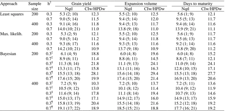
Regardless of the degree of dominance, heritability, and sample size, the least
squares and maximum likelihood approaches were equivalent for the number of
declared QTLs and confidence interval width (Table 1), the power of QTL detection and
number of false-positives (Tables 2 and 3), the bias between estimated and true QTL
positions (Table 4), and the estimates of genetic variances and percentage of the
phenotypic variance explained by each QTL (Table 5). Irrespective of the degree of
dominance, the number of declared QTLs was proportional to the heritability and
sample size. The average number of declared QTLs ranged from approximately 5, with
a heritability of 0.3 and 200 individuals, to 14, with a heritability of 0.7 and 400
individuals (Table 1). The confidence interval width was unaffected by the heritability
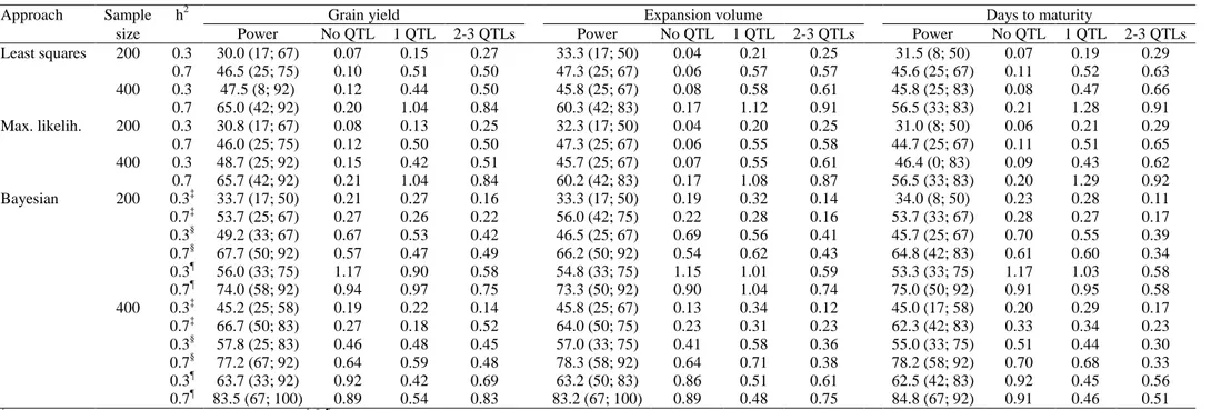
and sample size, showing an average value of 11.6 cM. The power of QTL detection
and the number of false-positives were highly influenced by the heritability and sample
size. The average power of QTL detection ranged from approximately 30%, for a
heritability of 0.3 and 200 individuals, to 66%, for a heritability of 0.7 and 400
individuals (Table 2).
Regardless of the degree of dominance, in general false-positives were mainly
declared in chromosomes with at least one true QTL, ranging from one false-positive
each eight chromosomes with one or more QTLs, assuming low heritability and 200
individuals, to one false-positive for each chromosome with one or more QTLs, with
high heritability and 400 individuals (Table 2). Under high heritability, one
false-positive for every 17 or five chromosomes with zero QTL were also declared,
12
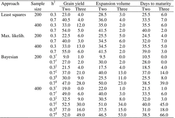
proportional to the heritability and sample size, reaching 55% under high heritability
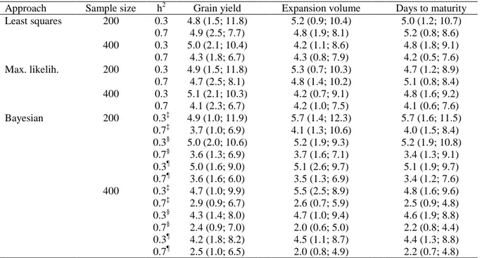
and 400 individuals (Table 3). The power of detection of three QTLs was low (5% on
average). The bias in the estimated QTL position was not affected by the degree of
dominance, heritability, and sample size, with an average value of 4.7 cM (Table 4). In
general, both methods provided underestimation of the additive variance and
overestimation of the dominance variance (60% on average) (Table 5). With respect to
the variance explained by each QTL, there was overestimation under smaller sample
size and low heritability, and underestimation with larger sample size and high
heritability, although the variance explained by all estimated QTLs agreed with the
parametric values (25 and 50%).
3.2.Bayesianapproach
The efficiency of Bayesian QTL mapping was not influenced by the degree of
dominance. However, the number of declared QTLs and the highest probability density
(HPD) region width (Table 1), the power of QTL detection, the number of
false-positives, and the power of simultaneous detection of QTLs (Tables 2 and 3), the bias in
the estimated QTL position (Table 4), and the bias in the estimated genetic variances
and in the percentage of the phenotypic variance explained by each QTL (Table 5) were
affected by the heritability, sample size, and prior expected number of QTLs. Increasing
the prior expected number of QTLs from 4 to 12 increased the number of declared QTLs from approximately 6-7 to 15-16, under low heritability, and from approximately
9-10 to 17-19, under high heritability, depending on the sample size (Table 1).
Increasing the heritability from 0.3 to 0.7 incremented the number of declared QTLs by
approximately 9 to 47%. The increase in the sample size from 200 to 400 caused an
13
increasing the prior expected number of QTLs, the HPD region width increased by approximately 7 to 98%, depending on the other two factors. This increase was due to
the identification of more than one QTL in the HPD region. In general, increasing the
heritability or the sample size decreased the HPD region width. The decreases ranged
from 4 to 39% and 5 to 45%, respectively. The HPD region width ranged from
approximately 10 to 29 cM (average 18.1).
The power of QTL detection was proportional to the prior expected number of QTLs, heritability, and sample size (Table 2). Changing the prior number of QTLs from
4 to 12 increased the power of QTL detection from approximately 33 to 85%,
depending on the heritability and sample size. The increment in the power of QTL
detection caused by increased heritability and sample size varied from approximately 31
to 68% and from 13 to 37%, respectively. However, the increase in the power of QTL
detection was followed by an increase in the number of false-positives. Regardless of
the sample size and heritability, and assuming 12 as the prior number of QTLs, there was one positive for each chromosome with only minor genes and one
false-positive for each one to two chromosomes with one or more true QTLs. The power of
simultaneous detection of two and three QTLs was proportional to the prior number of
QTLs, heritability, and sample size, ranging from 9 to 52.5% and from 0 to 66%,
respectively (Table 3).
The bias between the estimated and true positions of identified QTLs decreased
with increasing heritability, prior expected number of QTLs, and sample size (Table 4).
The decreases ranged from approximately 24 to 57%, 3 to 23%, and 3 to 46%,
respectively. The average bias ranged from approximately 5-6 cM assuming 200
14
size, heritability, and prior number of QTLs, the Bayesian analysis provided overestimation of the additive variance (the bias ranged from 19 to 54.5%) and, in
general, underestimation of the dominance variance (the bias ranged from
approximately −2 to −41%), for grain yield and expansion volume (Table 5). With
respect to days to maturity, generally the dominance variance estimates were close to
zero. The percentage of the phenotypic variance explained by each QTL was
proportional to the heritability and inversely proportional to the prior expected number
of QTLs and sample size. Generally, there was overestimation of the variance explained
by each QTL. The bias ranged from −5 to 180%.
3.3.Factors affecting the QTL mapping efficiency
Compared to the analysis assuming low density (one SNP each 10.9 cM),
increasing the marker density by 10 times provided an increase in the power of QTL
detection and in the mapping precision, especially for the least squares approach (Table
2, 3, 4, and 6). The increment in the power of QTL detection ranged from 10 to 23% for
the least squares approach, but from 1 to 7% for the Bayesian analysis. The increases in
the power of detection of two and three QTLs were also greater for the regression
analysis, compared to the Bayesian approach. The increase in the mapping precision
was higher for the Bayesian analysis. The decrease in the bias in the estimated QTL
position ranged from 16 to 45%. Only for the Bayesian analysis the number of
false-positives decreased by increasing the marker density.
The most important factor affecting the QTL mapping efficiency is the QTL
effect. Increasing the proportion of the phenotypic variance explained by each QTL
(10%), and consequently decreasing the minor genes effects, provided higher power of
15
increase in the mapping precision, especially with the Bayesian analysis (Tables 2, 4,
and 6). Under high heritability, the QTL detection power of the Bayesian approach was
maximized (100%) irrespective of the sample size and prior number of QTLs, the bias
in the estimated QTL position ranged from 0.8 to 1.6 cM, and the average number of
false-positives evidenced one false QTL for each two to four chromosomes. Under
higher proportion of the phenotypic variance explained by each QTL, the Bayesian QTL
16
4. Discussion
Based on relevant papers on QTL mapping efficiency (Zheng, 1994; Haley and
Knott, 1992; Lander and Botstein, 1989), our prior expectation was that QTL mapping
would prove to be highly efficient, i.e., it would provide a high power of QTL detection,
no false-positives but eventually some ghost QTLs (Martinez and Curnow, 1992), a
precise mapping of the QTLs underlying the trait, and slightly biased estimates of QTL
effects and variances. This was partially confirmed by our study. Our study shares some
similarities, such as the magnitude of the QTL effects and variances, and some
differences, such as greater number of minor genes and markers, with the
above-mentioned important papers. In the cited papers, the power of QTL detection ranged
from 40 (Zeng, 1994) to 80% (Lander and Botstein, 1989), from analyses based on
interval mapping, regression analysis, and composite interval. Lander and Botstein
(1989) did not declare QTLs in chromosomes with no genes.
The precision of the QTL mapping obtained in these three studies is impressive,
with bias ranging generally from 0 to 4 cM. The agreement between magnitude and the
sign of the estimated and true QTL effects and variances is also impressive. Most of our
results agree with these previous findings, including the equivalence between interval
mapping and regression analysis (Haley and Knott, 1992). Kao (2000) showed that the
least squares and maximum likelihood approaches could differ when the proportion of
the phenotypic variance explained by the QTLs and the marker interval increase, when
the differences among the QTL effects are larger, when epistasis between QTLs is
stronger, and when the QTLs are close. He concluded that interval mapping is more
accurate, precise, and powerful than regression analysis. However, Bogdan and Doerge
(2005) showed that the estimates of QTL locations and effects resulting from interval
17
concluded that the QTL detection power increased and the false-discovery rate
decreased, as the sample size increased, especially for larger-effect QTLs.
Assuming lower QTL effects, the QTL mapping of real data based on least
squares, maximum likelihood, or Bayesian analysis could not identify all the QTLs
underlying the trait and could declare a false QTL in chromosomes with one or more
true QTLs, especially under high heritability and sample size. In addition, the QTL
mapping could have a bias of 4-6 cM on average, and could underestimate or
overestimate the variance explained by each QTL, especially the least squares and
maximum likelihood approaches. The problem of false-positives could be worse with
Bayesian analysis, because false-positives can also be declared in chromosomes with no
QTL. Van Ooijen (1999) considered that real QTL mapping might contain
false-positive QTLs at too high a rate. Wang et al. (2012) showed that the bias in the
estimated QTL location decreases as the population size, QTL effect, or marker density
increases.
In comparison with the least squares and maximum likelihood approaches, the
Bayesian analysis showed generally greater power of QTL detection regardless of the
heritability, sample size, prior expected number of QTLs, marker density, and QTL effect. Under high density, the superiority ranged from approximately 2%, with high
heritability, 400 individuals, and four prior QTLs, to 87%, with low heritability, 200 individuals, and 12 prior QTLs. Under low density the superiority ranged from 46 to 100%, also inversely proportional to the heritability and sample size. With respect to
mapping precision, the Bayesian analysis provided less biased estimated QTL position.
Compared to the other approaches, the bias was 2 to 58% lower. Under high density,
18
higher power of detection of three QTLs. In the case of low density, the Bayesian QTL
mapping showed greater power of simultaneous detection of two and three QTLs
compared with the regression method.
However, the average number of false-positives in chromosome with no QTL was
greater for the Bayesian QTL mapping. The Bayesian analysis tended to declare one
false-positive for every eight chromosomes with no QTL to one false-positive for each
chromosome, depending on the heritability, sample size, prior expected number of QTLs, marker density, and QTL effect. With respect to the control of the type I error for
chromosomes with one or more QTLs, the Bayesian approach tended to be superior to
the regression method only with greater sample size and marker density. Increasing the
QTL effect tended to decrease the number of false-positives based on the Bayesian
analysis. In the absence of dominance, the Bayesian analysis provided generally no
relevant dominance effects and variances, fitting the additive-dominance model.
Nevertheless, the least squares and maximum likelihood approaches computed
significant dominance effects and variances. Fortunately, fitting a wrong model did not
affect the QTL mapping efficiency because in an F2 generation the additive and
dominance effects are not correlated.
Li et al. (2010) observed that interval mapping tends to overestimate a QTL
effect, especially for minor QTLs. From the Bayesian analysis of simulated backcross
data, assuming normally distributed phenotypes, Yang et al. (2009) observed an average
power of QTL detection of 49.5 and 64%, with sample sizes of 150 and 300,
respectively. The type I error rates were 6 and 4%. Mayer (2005) analyzed F2 simulated
data using regression analysis. The power of detection of two QTLs separated by 10 cM
ranged from 30 to 97%, being proportional to the sample size and inversely proportional
19
inversely proportional to the sample size and marker interval. Sisson and Hurn (2004)
employed Bayesian QTL mapping for the analyses of simulated F2 and real backcross
data, and produced contrasting results. The power of QTL detection was 100% for the
simulated data, with true locations generally correctly identified. However, the value
was only 40% for the real data, compared with previous analyses. Stephens and Fisch
(1998) analyzed simulated F2 data employing Bayesian analysis and composite interval
mapping. The powers of detection were 25 and 37.5%, respectively, and both analyses
declared one false-positive in a chromosome with no QTL. The biases in the estimated
QTL position were 2, 6, and 42 cM.
Breeders should not think that the need to specify the prior expected number of
QTLs in a Bayesian analysis is a problem. They can use the results from previous
studies or from an initial analysis based on interval mapping or regression analysis, or
define the value have in mind that an overestimation of the prior number of QTLs will
maximize the power of QTL detection and the number of false-positives. However,
false-positives can also occur when the prior number of QTLs is underestimated or incorrectly attributed. Furthermore, Bayesian QTL mapping and the available software
are accessible to breeders, as are regression and interval mapping methods and software.
The output and interpretation are very similar. Uimari et al. (1996) and Sillanpää and
Arjas (1998) highlighted some advantages of Bayesian QTL mapping, such as
incorporation of pedigree information, prior knowledge about unobserved quantities, uncertainty associated with fixed effects, variance components, marker allele
frequencies, and distances, and the relative ease by which missing data is handled.
Finally, it is important to highlight that a real QTL mapping can be slightly more
efficient than the efficiency evidenced in this simulation study. The R packages qtl, eqtl
20
QTL detection and decrease the number of false-positives and the bias between the
estimated and true QTL effects and variances. An alternative procedure that can
increase the QTL detecting power is the multiple-trait QTL mapping, especially with
highly correlated traits and pleiotropic QTLs (Fang et al., 2008; Knott and Haley, 2000;
21
5. Acknowledgments
We thank the National Council for Scientific and Technological Development (CNPq),
the Brazilian Federal Agency for Support and Evaluation of Graduate Education
(Capes), the Foundation for Research Support of Minas Gerais State (Fapemig), and
The World Academy of Sciences (TWAS) for financial support.
6. References
Bogdan, M., and R.W. Doerge. 2005. Biased estimators of quantitative trait locus
heritability and location in interval mapping. Heredity 95:476-484.
Broman, K.W., H. Wu, S. Sen, and G.A. Churchill. 2003. R/qtl: QTL mapping in
experimental crosses. Bioinformatics 19:889-890.
Fang, M., D. Jiang, L.J. Pu, H.J. Gao, P. Ji, H.Y. Wang, and R.Q. Yang. 2008.
Multitrait analysis of quantitative trait loci using Bayesian composite space
approach. BMC Genet. 9:48.
Foiada, F., P. Westermeier, B. Kessel, M. Ouzunova, V. Wimmer, W. Mayerhofer, T.
Presterl, M. Dilger, R. Kreps, J. Eder, and C.-C. Schön. 2015. Improving
resistance to the European corn borer: a comprehensive study in elite maize using
QTL mapping and genome-wide prediction. Theor. Appl. Genet. 128:875-891.
Haley, C.S., and S.A. Knott. 1992. A simple regression method for mapping
quantitative trait loci in line crosses using flanking markers. Heredity 69:315-324.
Jiang, C., and Z.B. Zeng. 1995. Multiple trait analysis of genetic mapping for
quantitative trait loci. Genetics 140:1111-1127.
Kao, C.-H. 2000. On the differences between maximum likelihood and regression
22
Kass, R.E., and A.E. Raftery. 1995. Bayes factors. J. Am. Stat. Assoc. 90:773-795.
Khalili, A.A., and O. Loudet. 2014. Package ‘eqtl’. cran.r-project.org.
Knott, S.A., and C.S. Haley. 2000. Multitrait least squares for quantitative trait loci
detection. Genetics 156:899-911.
Ku, L., L. Cao, X. Wei, H. Su, Z. Tian, S. Guo, L. Zhang, Z. Ren, X. Wang, Y. Zhu, G.
Li, Z. Wang, and Y. Chen. 2015. Genetic dissection of internode length above the
uppermost ear in four RIL populations of maize (Zea mays L.). G3-Genes
Genomes Genet. 5:281-289.
Lander, E.S., and D. Botstein. 1989. Mapping Mendelian factors underlying quantitative
traits using RFLP linkage maps. Genetics 121:185-199.
Li, H., S. Hearne, M. Bänziger, Z. Li, and J. Wang. 2010. Statistical properties of QTL
linkage mapping in biparental genetic populations. Heredity 105:257-267.
Martinez, O., and R.N. Curnow. 1992. Estimating the locations and the sizes of the
effects of quantitative trait loci using flanking markers. Theor. Appl. Genet.
85:480-488.
Mayer, M. 2005. A comparison of regression interval mapping and multiple interval
mapping for linked QTL. Heredity 94:599-605.
Nobari, K., M.R. Nassiry, A.A. Aslaminejad, M. Tahmoorespur, and A.K.
Esmailizadeh. 2012. Effects of QTL parameters and marker density on efficiency
of Haley-Knott regression interval mapping of QTL with complex traits and use
of artificial neural network for prediction of the efficiency of HK method in
livestock. J. Appl. Anim. Res. 40:247-255.
Qiu, H., X. Mei, C. Liu, J. Wang, G. Wang, X. Wang, Z. Liu, and Y. Cai. 2013. Fine
mapping of quantitative trait loci for acid phosphatase activity in maize leaf under
23
Sillanpää, M.J., and E. Arjas. 1998. Bayesian mapping of multiple quantitative trait loci
from incomplete inbred line cross data. Genetics 148:1373-1388.
Sisson, S.A., and M.A. Hurn (2004) Bayesian point estimation of quantitative trait loci.
Biometrics 60:60-68.
Spiegelhalter, D.J., N.G. Best, B.P. Carlin, and A. van der Linde. 2002. Bayesian
measures of model complexity and fit. J. R. Stat. Soc. B 64:583-639.
Stephens, D.A., and R.D. Fisch. 1998. Bayesian analysis of quantitative trait locus data
using reversible jump Markov chain Monte Carlo. Biometrics 54:1334-1347.
Teng, F., L. Zhai, R. Liu, W. Bai, L. Wang, D. Huo, Y. Tao, Y. Zheng, and Z. Zhang.
2013. ZmGA3ox2, a candidate gene for a major QTL, qPH3.1, for plant height in
maize. The Plant J. 73:405-416.
Uimari, P., G. Thaller, and I. Hoeschele. 1996. The use of multiple markers in a
Bayesian method for mapping quantitative trait loci. Genetics 143:1831-1842.
Van Ooijen, J.W. 1999. LOD significance thresholds for QTL analysis in experimental
populations of diploid species. Heredity 83:613-624.
Viana, J.M.S., M.S.F. Valente, F.F. Silva, G.B. Mundim, and G.P. Paes. 2013. Efficacy
of population structure analysis with breeding populations and inbred lines.
Genetica 141:389-399.
Yandell B.S., T. Mehta, S. Banerjee, D. Shriner, R. Venkataraman, J.Y. Moon, W.W.
Neely, H. Wu, R. von Smith, and N. Yi. 2007. R/qtlbim: QTL with Bayesian
Interval Mapping in experimental crosses. Bioinformatics 23:641-643.
Yang, R., X. Wang, J. Li, and H. Deng. 2008. Bayesian robust analysis for genetic
24
Wang, X., H. Gilbert, C. Moreno, O. Filangi, J.-M. Elsen, and P. L. Roy. 2012.
Statistical properties of interval mapping methods on quantitative trait loci
location: impact on QTL/eQTL analyses. BMC Genet. 13:29.
25
Table 1. Average number of QTLs† (Nqtl) and 95% confidence interval or highest probability density region width (CIw/HPDw) for the QTL position, from the least squares, maximum likelihood, and Bayesian approaches, regarding three traits, two heritabilities, and two sample sizes
Approach Sample h2 Grain yield Expansion volume Days to maturity
size Nqtl CIw/HPDw Nqtl CIw/HPDw Nqtl CIw/HPDw
Least squares 200 0.3 5.3 (2; 10) 12.3 5.5 (2; 10) 12.5 5.6 (1; 9) 12.1
0.7 9.0 (5; 14) 11.5 9.4 (5; 14) 12.0 9.5 (5; 13) 11.7
400 0.3 9.1 (4; 16) 11.8 9.4 (5; 13) 11.7 9.4 (6; 14) 11.6
0.7 14.0 (10; 21) 11.0 13.8 (9; 18) 11.0 13.9 (9; 21) 11.1
Max. likelih. 200 0.3 5.3 (2; 9) 12.1 5.5 (2; 10) 12.5 5.6 (1; 9) 11.7
0.7 9.0 (5; 14) 11.2 9.4 (5; 14) 11.8 9.5 (6; 13) 11.7
400 0.3 9.3 (6; 17) 11.6 9.3 (5; 13) 11.6 9.2 (1; 14) 11.6
0.7 14.2 (10; 21) 10.9 13.7 (9; 18) 10.9 13.8 (9; 20) 11.2
Bayesian 200 0.3‡ 6.1 (4; 9) 18.8 6.0 (4; 8) 19.6 6.0 (4; 8) 15.2
0.7‡ 8.9 (6; 11) 11.4 8.8 (6; 11) 14.5 8.8 (7; 11) 12.1
0.3§ 11.3 (8; 14) 21.8 11.1 (9; 13) 24.1 11.0 (9; 14) 24.1 0.7§ 13.3 (11; 17) 15.8 13.1 (11; 16) 16.3 12.8 (10; 15) 17.1 0.3¶ 15.5 (13; 18) 28.1 15.6 (14; 18) 29.4 15.5 (13; 18) 27.7 0.7¶ 17.6 (15; 20) 19.9 17.4 (15; 20) 21.4 16.9 (13; 20) 20.6
400 0.3‡ 7.2 (5; 9) 10.3 7.2 (5; 10) 13.7 7.2 (5; 11) 13.6
0.7‡ 10.5 (9; 12) 13.0 10.1 (8; 12) 11.4 10.4 (9; 12) 11.9 0.3§ 11.6 (9; 14) 17.8 11.1 (8; 14) 19.4 10.7 (9; 13) 14.6 0.7§ 15.0 (13; 17) 17.1 14.9 (12; 17) 16.0 14.9 (13; 17) 15.9 0.3¶ 15.8 (13; 19) 20.4 15.5 (14; 18) 21.6 15.2 (12; 18) 19.2 0.7¶ 19.1 (17; 22) 18.9 18.5 (15; 21) 18.8 17.7 (16; 21) 19.2
†
26
Table 2. Average power of QTL detection† (%) and number of false QTLs in chromosomes with zero, one, and two to three true QTLs, from the least squares, maximum likelihood, and Bayesian approaches, regarding three traits, two heritabilities, and two sample sizes
Approach Sample h2 Grain yield Expansion volume Days to maturity
size Power No QTL 1 QTL 2-3 QTLs Power No QTL 1 QTL 2-3 QTLs Power No QTL 1 QTL 2-3 QTLs
Least squares 200 0.3 30.0 (17; 67) 0.07 0.15 0.27 33.3 (17; 50) 0.04 0.21 0.25 31.5 (8; 50) 0.07 0.19 0.29 0.7 46.5 (25; 75) 0.10 0.51 0.50 47.3 (25; 67) 0.06 0.57 0.57 45.6 (25; 67) 0.11 0.52 0.63 400 0.3 47.5 (8; 92) 0.12 0.44 0.50 45.8 (25; 67) 0.08 0.58 0.61 45.8 (25; 83) 0.08 0.47 0.66 0.7 65.0 (42; 92) 0.20 1.04 0.84 60.3 (42; 83) 0.17 1.12 0.91 56.5 (33; 83) 0.21 1.28 0.91 Max. likelih. 200 0.3 30.8 (17; 67) 0.08 0.13 0.25 32.3 (17; 50) 0.04 0.20 0.25 31.0 (8; 50) 0.06 0.21 0.29 0.7 46.0 (25; 75) 0.12 0.50 0.50 47.3 (25; 67) 0.06 0.55 0.58 44.7 (25; 67) 0.11 0.51 0.65 400 0.3 48.7 (25; 92) 0.15 0.42 0.51 45.7 (25; 67) 0.07 0.55 0.61 46.4 (0; 83) 0.09 0.43 0.62 0.7 65.7 (42; 92) 0.21 1.04 0.84 60.2 (42; 83) 0.17 1.08 0.87 56.5 (33; 83) 0.20 1.29 0.92 Bayesian 200 0.3‡ 33.7 (17; 50) 0.21 0.27 0.16 33.3 (17; 50) 0.19 0.32 0.14 34.0 (8; 50) 0.23 0.28 0.11 0.7‡ 53.7 (25; 67) 0.27 0.26 0.22 56.0 (42; 75) 0.22 0.28 0.16 53.7 (33; 67) 0.28 0.27 0.17 0.3§ 49.2 (33; 67) 0.67 0.53 0.42 46.5 (25; 67) 0.69 0.56 0.41 45.7 (25; 67) 0.70 0.55 0.39 0.7§ 67.7 (50; 92) 0.57 0.47 0.49 66.2 (50; 92) 0.54 0.62 0.43 64.8 (42; 83) 0.61 0.60 0.34 0.3¶ 56.0 (33; 75) 1.17 0.90 0.58 54.8 (33; 75) 1.15 1.01 0.59 53.3 (33; 75) 1.17 1.03 0.58 0.7¶ 74.0 (58; 92) 0.94 0.97 0.75 73.3 (50; 92) 0.90 1.04 0.74 75.0 (50; 92) 0.91 0.95 0.58 400 0.3‡ 45.2 (25; 58) 0.19 0.22 0.14 45.8 (25; 67) 0.13 0.34 0.12 45.0 (17; 58) 0.20 0.29 0.17 0.7‡ 66.7 (50; 83) 0.27 0.18 0.52 64.0 (50; 75) 0.23 0.31 0.23 62.3 (42; 83) 0.33 0.34 0.23 0.3§ 57.8 (25; 83) 0.46 0.48 0.45 57.0 (33; 75) 0.41 0.58 0.36 55.0 (33; 75) 0.51 0.44 0.30 0.7§ 77.2 (67; 92) 0.64 0.59 0.48 78.3 (58; 92) 0.64 0.71 0.38 78.2 (58; 92) 0.70 0.68 0.33 0.3¶ 63.7 (33; 92) 0.92 0.42 0.69 63.2 (50; 83) 0.86 0.51 0.61 62.5 (42; 83) 0.92 0.45 0.56 0.7¶ 83.5 (67; 100) 0.89 0.54 0.83 83.2 (67; 100) 0.89 0.48 0.75 84.8 (67; 92) 0.91 0.46 0.51
†
27
Table 3. Average power of simultaneous detection of two and three QTLs (%) from the
least squares, maximum likelihood, and Bayesian approaches, regarding three traits, two
heritabilities, and two sample sizes
Approach Sample h2 Grain yield Expansion volume Days to maturity
size Two Three Two Three Two Three
Least squares 200 0.3 23.0 4.0 28.5 3.0 25.5 6.0
0.7 40.5 4.0 36.0 4.0 33.5 7.0
400 0.3 33.0 12.0 35.0 2.0 35.5 6.0
0.7 54.0 5.0 41.5 2.0 40.0 2.0
Max. likelih. 200 0.3 22.5 6.0 25.5 5.0 24.5 4.0
0.7 40.0 3.0 34.5 6.0 32.0 7.0
400 0.3 33.0 13.0 34.5 2.0 35.5 5.0
0.7 55.0 6.0 41.5 2.0 39.0 3.0
Bayesian 200 0.3† 9.0 1.0 9.5 0.0 10.5 0.0
0.7† 27.0 2.0 30.0 2.0 28.0 0.0
0.3‡ 21.5 4.0 17.5 4.0 18.5 4.0
0.7‡ 37.0 21.0 40.0 13.0 37.0 14.0
0.3§ 30.0 9.0 25.5 11.0 25.5 8.0
0.7§ 47.0 28.0 50.0 23.0 38.5 39.0
400 0.3† 19.0 0.0 22.0 1.0 21.5 1.0
0.7† 49.0 6.0 40.0 3.0 33.5 6.0
0.3‡ 32.5 9.0 30.5 8.0 32.0 3.0
0.7‡ 52.5 30.0 51.0 34.0 40.0 45.0 0.3§ 37.0 16.0 37.5 15.0 31.0 18.0 0.7§ 52.0 49.0 46.5 53.0 38.5 66.0
28
Table 4. Average bias† (cM) in the estimated QTL position, from the least squares,
maximum likelihood, and Bayesian approaches, regarding three traits, two heritabilities,
and two sample sizes
Approach Sample size h2 Grain yield Expansion volume Days to maturity Least squares 200 0.3 4.8 (1.5; 11.8) 5.2 (0.9; 10.4) 5.0 (1.2; 10.7)
0.7 4.9 (2.5; 7.7) 4.8 (1.9; 8.1) 5.2 (0.8; 8.6) 400 0.3 5.0 (2.1; 10.4) 4.2 (1.1; 8.6) 4.8 (1.8; 9.1) 0.7 4.3 (1.8; 6.7) 4.3 (0.8; 7.9) 4.2 (0.5; 7.6) Max. likelih. 200 0.3 4.9 (1.5; 11.8) 5.3 (0.7; 10.3) 4.7 (1.2; 8.9) 0.7 4.7 (2.5; 8.1) 4.8 (1.4; 10.2) 5.1 (0.8; 8.4) 400 0.3 5.1 (2.1; 10.3) 4.2 (0.7; 9.1) 4.8 (1.6; 9.2) 0.7 4.1 (2.3; 6.7) 4.2 (1.0; 7.5) 4.1 (0.6; 7.6) Bayesian 200 0.3‡ 4.9 (1.0; 11.9) 5.7 (1.4; 12.3) 5.7 (1.6; 11.5)
0.7‡ 3.7 (1.0; 6.9) 4.1 (1.3; 10.6) 4.0 (1.5; 8.4) 0.3§ 5.0 (2.0; 10.6) 5.2 (1.9; 9.3) 5.2 (1.9; 10.8) 0.7§ 3.6 (1.3; 6.9) 3.7 (1.6; 7.1) 3.4 (1.3; 9.1) 0.3¶ 5.0 (1.6; 9.0) 5.1 (2.6; 9.7) 5.1 (1.9; 9.7) 0.7¶ 3.6 (1.6; 6.0) 3.5 (1.3; 6.9) 3.4 (1.2; 7.6) 400 0.3‡ 4.7 (1.0; 9.9) 5.5 (2.5; 8.9) 4.8 (1.6; 9.6) 0.7‡ 2.9 (0.9; 6.7) 2.6 (0.7; 5.9) 2.5 (0.9; 4.8) 0.3§ 4.3 (1.4; 8.0) 4.7 (1.0; 9.4) 4.6 (1.9; 8.8) 0.7§ 2.4 (0.9; 7.0) 2.0 (0.6; 5.0) 2.2 (0.8; 4.4) 0.3¶ 4.2 (1.8; 8.2) 4.5 (1.1; 8.7) 4.4 (1.3; 8.8) 0.7¶ 2.5 (1.0; 6.5) 2.0 (0.8; 4.9) 2.2 (0.7; 4.8)
29
Table 5. Average additive and dominance variances, and percentage of the phenotypic variance explained by each QTL† from the least squares, maximum likelihood and Bayesian approaches, regarding three traits, two heritabilities, and two sample sizes
Approach Sample h2 Grain yield Expansion volume Days to maturity
size Add. var. Dom. var. % explained Add. var. Dom. var. % explained Add. var. Dom. var. % explained Least squares 200 0.3 57.88 80.52 3.8 (2.8; 7.8) 4.69 5.69 4.0 (2.8; 8.0) 5.87 6.65 4.0 (2.7; 9.8)
0.7 44.36 60.20 3.6 (2.8; 7.9) 3.32 4.41 3.6 (2.8; 5.6) 4.66 5.58 3.7 (2.6; 7.4) 400 0.3 53.48 69.29 2.1 (1.6; 5.5) 4.01 4.94 2.0 (1.5; 3.9) 5.05 6.27 2.1 (1.6; 5.1) 0.7 41.10 50.01 1.9 (1.5; 3.4) 2.91 3.44 2.0 (1.4; 4.2) 3.70 4.28 2.0 (1.6; 4.0) Max. likelih. 200 0.3 63.46 80.15 3.9 (2.1; 8.1) 4.28 5.57 3.8 (2.7; 7.5) 5.03 6.48 3.7 (2.1; 9.2) 0.7 50.50 61.20 3.8 (2.6; 6.8) 3.34 4.34 3.5 (2.9; 6.2) 4.15 5.44 3.6 (2.6; 6.4) 400 0.3 67.11 72.85 2.2 (1.6; 6.7) 3.58 4.86 1.9 (1.5; 2.6) 4.17 5.65 4.4 (1.7; 9.7) 0.7 45.31 51.02 2.0 (1.5; 3.4) 2.93 3.66 2.1 (1.5; 8.5) 3.05 4.23 1.8 (1.6; 2.7) Bayesian 200 0.3‡ 153.67 37.96 4.9 (2.8; 9.2) 12.34 1.79 5.2 (3.2; 7.3) 17.23 0.88 5.6 (2.5; 8.9) 0.7‡ 154.28 37.76 6.8 (4.7; 10.7) 11.83 1.62 6.7 (5.3; 9.0) 16.91 0.22 6.9 (5.1; 8.8) 0.3§ 177.30 57.44 3.2 (2.1; 4.8) 13.65 2.96 3.3 (2.3; 4.9) 19.15 1.94 3.5 (2.3; 5.2) 0.7§ 161.23 45.60 4.8 (3.8; 6.3) 12.43 2.14 4.9 (3.8; 6.0) 17.76 0.42 5.1 (3.8; 6.1) 0.3¶ 196.32 74.85 2.7 (2.0; 4.1) 14.82 4.15 2.7 (2.0; 3.9) 20.78 3.11 2.8 (2.1; 3.8) 0.7¶ 167.69 50.84 3.8 (3.1; 4.9) 12.84 2.54 3.8 (3.2; 4.9) 18.35 0.66 4.0 (3.2; 5.2) 400 0.3‡ 166.24 37.96 4.2 (2.5; 6.2) 12.83 1.42 4.3 (3.0; 6.3) 18.20 0.35 4.7 (3.5; 6.8) 0.7‡ 153.97 42.18 5.7 (4.5; 7.2) 11.74 2.05 5.9 (4.6; 8.6) 16.78 0.06 5.6 (4.7; 6.9) 0.3§ 174.15 53.48 3.0 (2.3; 3.8) 13.58 2.10 3.1 (2.4; 3.9) 19.10 0.75 3.4 (2.6; 4.5) 0.7§ 166.85 45.40 4.3 (3.4; 6.3) 12.64 2.24 4.3 (3.5; 5.6) 18.34 0.13 4.3 (3.2; 5.2) 0.3¶ 184.74 62.74 2.4 (1.6; 2.9) 14.33 2.72 2.4 (2.0; 3.1) 20.02 1.22 2.5 (2.0; 3.1) 0.7¶ 169.88 47.40 3.4 (2.8; 4.4) 12.94 2.36 3.6 (3.0; 4.5) 18.60 0.21 3.7 (2.8; 4.7)
30
Table 6. Average number of QTLs (Nqtl), 95% confidence interval or high probability density region width (CIw/HPDw), power of QTL detection
(%), number of false QTLs in chromosomes with zero, one, and two to three true QTLs, power of simultaneous detection of two and three QTLs (%), bias (cM) in the estimated QTL position, and percentage of the phenotypic variance explained by each QTL, from the least squares and Bayesian approaches, regarding grain yield, two heritabilities, and two sample sizes
Approach Sample h2 Nqtl CIw/HPDw Power No QTL 1 QTL 2-3 QTLs Power 2 Power 3 Bias V(A) V(D) % explained
Least Squares 200 0.3† 4.3 15.9 27.2 0.04 0.08 0.19 20.0 3.0 6.1 62.05 87.19 5.1
0.7† 6.9 14.2 37.7 0.05 0.29 0.40 24.0 4.0 5.8 44.44 62.09 4.7
0.7‡ 9.7 12.0 90.8 0.04 0.67 - - - 2.8 126.56 124.81 4.1
400 0.3† 7.3 14.5 38.5 0.09 0.26 0.45 25.0 2.0 5.7 60.88 85.25 2.9
0.7† 11.3 13.4 53.7 0.14 0.92 0.60 32.5 3.0 5.0 45.04 65.50 2.8
0.7‡ 14.2 10.9 99.3 0.11 1.28 - - - 1.9 126.64 123.86 2.2
Bayesian 200 0.3†,# 16.7 31.6 54.7 1.26 1.19 0.67 33.0 9.0 6.3 265.29 146.31 3.6
0.7†,# 20.3 28.2 70.8 1.29 1.35 0.99 46.5 25.0 5.7 234.43 96.01 5.0
0.7‡,§ 7.2 4.5 99.0 0.14 0.12 - - - 1.6 286.58 68.09 9.5
0.7‡,¶ 12.0 5.3 100.0 0.50 0.66 - - - 1.5 290.62 76.18 5.9
400 0.3†,# 16.3 26.2 63.0 1.07 1.08 0.58 38.0 16.0 5.2 211.88 84.68 2.8
0.7†,# 20.5 26.4 78.3 1.14 1.34 0.97 50.0 38.0 4.5 234.49 77.85 4.7
0.7‡,§ 7.8 3.7 100.0 0.24 0.13 - - - 0.8 286.22 65.23 8.7
0.7‡,¶ 11.5 3.9 100.0 0.60 0.51 - - - 0.8 294.69 68.57 6.0
†
31
7. Appendix
Code for maximum likelihood and least squares approaches
setwd("C:/QTL mapping") library(qtl)
library(eqtl) thres=3
####reading map################# map=read.table("map.txt",skip = 1)
map=as.matrix(rbind(t(matrix(map$V2)),map$V1,round(map$V3,2)))
for(i in 1:50) {
####reading genotype##############
gen=read.table("sample 200.txt")[read.table("sample 200.txt")[,1]==i,][,-(1:2)] gen[gen==11]<-"A" gen[gen==12]<-"H" gen[gen==21]<-"H" gen[gen==22]<-"B" gen=as.matrix(gen) ####reading phenotype##############
fen=as.matrix(read.table("values ev 0.3 200.txt")[read.table("values ev 0.3 200.txt")[,2]==i,c(6)]) fen=c("Y"," "," ",fen)
####combining phe, map, and gen##### data=cbind(fen,rbind(map,gen))
write.table(data, "data.csv", col.names=F,row.names=F,quote=F, sep=",", dec=".")
dados= read.cross("csv", ".", "data.csv")
genoprob= calc.genoprob(dados, step=0.5 ,map.function=c("haldane"))
scan=scanone(genoprob, method="em") #hk:Haley-Knott; em: interval mapping (Lander and Botstein)
####chr1#################
p1=define.peak(scan,chr=1,lodcolumn=c(3),phe.name="Y",th=thres)$Y$`1`
if (is.na(p1)==FALSE) {nqtl<-nrow(p1)} else {nqtl<-0} if (nqtl>0)
{
qc=rep(1,nqtl) qp=p1$peak.cM
qtl= makeqtl(genoprob, qc, qp, what="prob")
lod = fitqtl(genoprob, pheno.col=1, qtl, method="hk",get.ests=TRUE) ef1 = matrix(lod$ests$ests[-1],nqtl,2,byrow=T)
colnames(ef1)=c("a","d")
var1 = matrix(diag(lod$ests$covar)[-1],nqtl,2,byrow=T) colnames(var1)=c("vara","vard")
result1=cbind(qc,p1,ef1,var1) }
32
... (same for chromosomes 2 to 9)
####chr10#################
p10=define.peak(scan,chr=10,lodcolumn=c(3),phe.name="Y",th=thres)$Y$`10`
if (is.na(p10)==FALSE) {nqtl<-nrow(p10)} else {nqtl<-0} if (nqtl>0)
{
qc=rep(10,nqtl) qp=p10$peak.cM
qtl= makeqtl(genoprob, qc, qp, what="prob")
lod = fitqtl(genoprob, pheno.col=1, qtl, method="hk",get.ests=TRUE) ef10 = matrix(lod$ests$ests[-1],nqtl,2,byrow=T)
colnames(ef10)=c("a","d")
var10 = matrix(diag(lod$ests$covar)[-1],nqtl,2,byrow=T) colnames(var10)=c("vara","vard") result10=cbind(qc,p10,ef10,var10) } else {result10<-NA} ####output################# tresult=na.omit(cbind(i,rbind(result1,result2,result3,result4,result5,result6,result7,result8,result9,result10)))[,-c(4,6,8,10)]
if (i==1) {result=tresult} else {result=rbind(result,tresult)}
write.table(result,"output ev 0.3 200 ml.txt",row.names=F,quote=F)
}
Code for Bayesian analysis
setwd("C:/QTL mapping") library(qtlbim)
#####reading map#####
map=read.table("map hp.txt",skip = 1)
map=as.matrix(rbind(t(matrix(map$V2)),map$V1,round(map$V3,2)))
for(i in 1:50) {
#####reading genotypes#####
gen=read.table("sample 400 hp.txt")[read.table("sample 400 hp.txt")[,1]==i,][,-(1:2)] gen[gen==11]<-"A" gen[gen==12]<-"H" gen[gen==21]<-"H" gen[gen==22]<-"B" gen=as.matrix(gen) #####reading phenotypes######
fen=as.matrix(read.table("values gy 0.7 400 hp.txt")[read.table("values gy 0.7 400 hp.txt")[,2]==i,c(6)]) fen=c("Y"," "," ",fen)
#####combining gen, map and phen##### data=cbind(fen,rbind(map,gen))
33
#####Bayesian analysis#####
crossobj <- read.cross("csv", ".", "data.csv")
qbgenoprob <- qb.genoprob(crossobj, map.funct="haldane", step=0.5, stepwidth = "variable") qbdata <- qb.data(crossobj, pheno.col = 1, trait = "normal", fixcov = 0, rancov = 0)
qbmodel <- qb.model(crossobj, epistasis = FALSE, main.nqtl = 8)
qbmcmc <- qb.mcmc(crossobj, qbdata, qbmodel, pheno.col = 1, seed = 1616) qbmm <- qb.mainmodes(qbmcmc, cutoff = 25)
qbho <- qb.hpdone(qbmcmc, level=0.475, effects = "estimate") qbvc <- qb.varcomp(qbmcmc, scan = "main")
aux1=cbind(qbmcmc$mcmc.samples$Y$mainloci$niter,qbmcmc$mcmc.samples$Y$mainloci$vardom) head(aux1)
NITER=unique(aux1[,1]) soma=NULL
for(j in 1:length(NITER)) {
soma[j]=sum(aux1[aux1[,1]==NITER[j],2]) }
#####output#####
tresult1 <- rbind(qbmm$nqtl.est,qbmm$peaks) tresult2 <- cbind(i,summary(qbho))
tresult3 <- cbind(i,summary(qbvc)) tresult4 <- mean(soma)
if (i==1) {result1=tresult1} else {result1=rbind(result1,tresult1)}
write.table(result1,"output gy 0.7 400 8 hp peak.txt",row.names=F,quote=F)
if (i==1) {result2=tresult2} else {result2=rbind(result2,tresult2)}
write.table(result2,"output gy 0.7 400 8 hp hpd.txt",row.names=F,quote=F)
if (i==1) {result3=tresult3} else {result3=rbind(result3,tresult3)}
write.table(result3,"output gy 0.7 400 8 hp vc.txt",row.names=F,quote=F)
if (i==1) {result4=tresult4} else {result4=rbind(result4,tresult4)}
write.table(result4,"output gy 0.7 400 8 hp vd.txt",row.names=F,quote=F)