Binomial-exponential 2 Distribution:
Different Estimation Methods with Weather Applications
H.S. BAKOUCH1, S. DEY2, P.L. RAMOS3* and F. LOUZADA3
Received on September 8, 2016 / Accepted on May 13, 2017
ABSTRACT.In this paper, we have considered different estimation methods of the unknown parameters of a binomial-exponential 2 distribution. First, we briefly describe different methods of estimation such as maximum likelihood, method of moments, percentile based estimation, least squares, method of maximum product of spacings, method of Cram´er-von-Mises, methods of Darling and right-tail Anderson-Darling, and compare them using extensive simulations studies. Finally, the potentiality of the model is studied using three real data sets related to the total monthly rainfall during April, May and September at S˜ao Carlos, Brazil.
Keywords: binomial-exponential 2, maximum likelihood estimation, Cram´er-von-Mises type minimum distance estimators, right-tail Anderson-Darling estimators.
1 INTRODUCTION
The binomial-exponential 2 (B E2) distribution has been introduced by Bakouch et al. [6] as a distribution of a random sum of independent exponential random variables when the sample size has a zero truncated binomial distribution. TheB E2 distribution has the probability density function (pdf)
f(x;θ , λ)=
1+(λx−1) θ
2−θ
λe−λx, (1.1)
and the cumulative distribution function (cdf)
F(x;θ , λ)=1−
1+ λθx
2−θ
e−λx, (1.2)
where 0≤θ≤1 is the shape parameter andλ >0 is the scale parameter. TheB E2 distribution has an increasing and constant failure rate property. A generalization of the BE2 distribution was discussed by Asgharzadeh et al. [4].
*Corresponding author: Pedro Luiz Ramos – E-mail: [email protected]
Bakouch et al. [6] in their paper only considered the maximum likelihood estimation (MLE) method to estimate the parameters of the BE2 distribution. However it is of interest to compare the MLE method with other estimation procedures such as the method of moments, ordinary least-squares estimation (OLSE), weighted least-squares estimation (WLSE), percentile estima-tion (PCE), maximum product of spacings estimaestima-tion (MPS), Cram´e r-von-Mises type minimum distance estimation (CME), Anderson-Darling (ADE) and Right-tail Anderson-Darling estima-tion (RADE).
We have several estimation methods available for the parametric distribution in the literature, some of the estimation methods are well researched on theoretical aspect. However, it is worth noting that in the case of small samples, there is often evidence that the maximum likelihood method does not perform well. Therefore, other estimating methods have recently been devel-oped. The appeal of the estimation methods vary from user to user and area of application. For instance, one may prefer to use the moment estimator even when it does not have a closed form expression. The objective of the article is to develop a guideline for choosing the best estimation method for the BE2 distribution, which would be of interest to applied statisticians. Compar-isons of estimation methods for other distributions have been investigated in the literature, see e.g., [1, 5, 11, 13, 17, 19, 21, 26].
The main goal of this paper is two fold: First is to show how different frequentist estimators of the proposed distribution perform for different sample sizes and second is to show that the distribution outperforms at least two-parameter distributions with respect to three real data sets.
Other motivation to use the BE2 distribution comes from the fact that stochastic models that accommodate zero value has vast importance in practical applications, for example in forecast models when we observe the monthly rainfall precipitation, it is common in dry periods the non occurrence of precipitation, therefore the occurrence of zero value can be observed in differ-ent measures such as the average, maximum and minimum. Popular models such as Gamma, Weibull, Lognormal and Generalized Exponential distributions do not accommodate such char-acteristic. In this paper we demonstrate that the BE2 distribution allows the occurrence of zero value, becoming a simple alternative to be used in weather forecast models.
The paper is organized as follows. In Section 2, we present some notes and properties for the model. In Section 3, we discuss the nine estimation methods considered in this paper. In Section 4 a simulation study is presented in order to identify the most efficient estimators. In Section 5 we apply our proposed methodology to three real data sets related to the total monthly rainfall during April, May and September at S˜ao Carlos, Brazil. Finally in Section 6 we conclude the paper.
2 NOTES AND PROPERTIES
distribution (with shape 2 and scaleλ), i.e. f(x;p, λ)=pλ2xe−λx+(1−p)λe−λx, where the mixing proportionp=2−θθ.
LetX∼B E2(θ , λ), the raw moments ofX about the origin is given by
E(Xr)= r!
λr
1+ rθ
2−θ
, (2.1)
and the survival function ofX is given by
S(x;θ , λ)=
1+ λθx
2−θ
e−λx.
Many distributions such as Gamma, Weibull, Lognormal, to list a few, do not allow occurrence of zero values. The following proposition prove that the BE2 distribution can be used as a model with occurrence of zero value.
Proposition 2.1.Let X be a random variable with BE2 distribution then fX(0;θ , λ)≥0for all
0≤θ≤1andλ >0.
Proof. Note that
fX(0;θ , λ)=
d
d xFX(x;θ , λ)
0=
2−2θ
2−θ
λ (2.2)
where fX(0;θ , λ)≥0 for all 0≤θ≤1 andλ >0.
This result allows us to use the BE2 distribution as a simple alternative in the problems with occurrence of zero value.
3 METHODS OF ESTIMATION
In this section, nine estimation procedures are discussed to obtain the estimates of the BE2 distribution parameters.
3.1 Maximum Likelihood Estimation
The method of maximum likelihood is the most frequently used method of parameter estimation. The method’s success stems no doubt from its many desirable properties including consistency, asymptotic efficiency, normality, invariance and simply its intuitive appeal. Letx1, . . . ,xnbe a
random sample of sizenfrom (1.1), the likelihood function of the density (1.1) is given by
L(θ , λ;x)= n
i=1
f(xi, θ , λ)=λnexp
−λ
n
i=1
xi
n
i=1
1+(λxi −1)θ
2−θ
(3.1)
The log-likelihood function without constant terms is given by
ℓ(θ , λ;x)=nlogλ−λ
n
i=1
xi−nlog(2−θ )+ n
i=1
From the expressions∂θ∂l(θ , λ;x)=0, ∂
∂λl(θ , λ;x)=0, the likelihood equations are
n λ−
n
i=1
xi+ n
i=1
θxi
(2−2θ+λθxi)
=0 (3.3)
and
n
2−θ +
n
i=1
λxi−2
2−2θ+λθxi
=0. (3.4)
The maximum likelihood estimatorθˆandλˆare obtained by solving the non-linear equations (3.3) and (3.4). It is important to point out that, non-linear optimization algorithms such as the quasi-Newton algorithm, can be used to maximize directly the likelihood function given in (3.1).
3.2 Moments Estimators
The method of moments is fairly simple procedure and has been widely used for estimating parameters in statistical models. The moments estimators (MEs) of the BE2 distribution can be obtained by equating the theoretical moments of (1.1) with the sample moments. Consider that
E(X|θ , λ)= 2
λ(2−θ ) and V ar(X|θ , λ)=
2(2−θ2)
λ2(2−θ )2· (3.5)
are the theoretical moments of the BE2 distribution. Note that, the population coefficient of variation given by
CV(X|θ , λ)= 2(2−θ 2)
2
is independent of the scale parameterλ. So, the estimatorθˆM M E forθandλˆM M E forλ, can be
easily obtained by solving
ˆ
θM M E =
2−2
s
¯
x
2
, and
ˆ
λM M E =
2
¯
x
2−
2−2sx¯2
(3.6)
wherex¯andsare the sample mean and sample standard deviation respectively.
3.3 Least-Square Estimators
The ordinary least square and the weighted least square are well known methods used for estimat-ing the unknown parameters [25]. Let F(x)be the distribution function of the random variables
{X1,X2, . . . ,Xn}andX(1)<X(2)<· · ·<X(n)be ordered random variables. The least square
estimators ofθandλ, denoted byθˆL S EandλˆL S Ecan be obtained by minimizing the function
LS(θ , λ)= n
i=1
Fx(i)|θ , λ
− i
n+1
2
with respect toθ andλ, where F(·)is given by (1.2). Equivalently, they can be obtained by solving the following non-linear equations:
n
i=1
Fx(i)|θ , λ
− i
n+1
η1
x(i)|θ , λ
=0,
n
i=1
Fx(i)|θ , λ
− i
n+1
η2
x(i)|θ , λ
=0.
Consider the following weighted function (see Gupta & Kundu [13])
wi =
1 Var(F(x(i)))
= (n+1) 2(n+
2) i(n−i+1) .
The WLSEs,θW L S EandλW L S E, can be obtained by minimizing
WLS(θ , λ)= n
i=1
(n+1)2(n+2) i(n−i+1)
Fx(i)|θ , λ−
i n+1
2
. (3.8)
These estimators can also be obtained by solving:
n
i=1
(n+1)2(n+2) i(n−i+1)
Fx(i) |θ , λ
− i
n+1
η1
x(i) |θ , λ
=0,
n
i=1
(n+1)2(n+2) i(n−i+1)
Fx(i) |θ , λ
− i
n+1
η2
x(i) |θ , λ
=0,
where
η1
x(i)|θ , λ
= −2λx(i)e
−λx(i)
(2−θ )2 , (3.9)
and
η2
x(i)|θ , λ
=x(i)e−λx(i)(1+
λθx(i)
2−θ)−
θx(i)e−λx(i)
2−θ . (3.10)
3.4 Percentile Estimators
The percentile estimators is originally suggested by Kao [15,16]. This method is commonly used to estimate the unknown parameters from the distribution functions that has a closed form of the quantile function. The percentile estimates (PCEs) can be obtained by minimizing with respect unknown parameters, the Euclidean distance between the ordered sample points and ordered theoretical points, computed throughout the quantile function. Since,
F(x, θ , λ)=1−
1+ λθx
2−θ
therefore, the quantile function is given by
xp=
1
λlog
2−θ+λθxp
(2−θ ) (1−p)
.
LetX(j)be thejth order statistics, i.e.,X(1)<X(2)<· · ·<X(n). Ifpjdenotes some estimators
ofF(x(j);θ , λ), then the estimators ofθandλcan be obtained by minimizing
n
j=1
x(j)−
1
λln
2−θ+λθxp
(2−θ )1−pj
2
(3.11)
with respect toθ andλ. The percentile estimatorsθˆPC E andλˆPC E can be obtained by solving
the following nonlinear equations
n
j=1
xj−
1 λlog
(2−θ+λθx p (2−θ )(1−pj)
xp
(2−θ+λθxp)(2−θ ))
=0,
n
j=1
xj−
1 λlog
(2−θ+λθx p (2−θ )(1−pj)
1 λ2log
(2−θ+λθxp) (2−θ )(1−pj)
− 1 λ
θxp (2−θ+λθxp)
=0,
respectively. In this paper, we consider the estimator of pj as pj = n+1j . However, different estimators can be used instead, see for example Mann, et al. (1974).
3.5 Method of Maximum Product of Spacings
The maximum product spacing (MPS) method has been introduced by Cheng & Amin [9] as an alternative to MLE for the estimation of the unknown parameters of continuous univariate distri-butions. The MPS method was also derived independently by Ranneby [22] as an approximation to the Kullback-Leibler measure of information. This method is as efficient as the MLE estima-tors and consistent under more general conditions. Using the same notations in subsection 3.3, define the uniform spacings of a random sample from the BE2 distribution as:
Di(θ , λ)=F(xi:n|θ , λ)−F(xi−1:n|θ , λ) , i =1,2, . . . ,n,
whereF(x0:n|θ , λ)=0 andF(xn+1:n |θ , λ)=1. Clearlyni=1+1Di(θ , λ)=1.
The maximum product of spacings estimatorsθM P S andλM P S, of the parametersθ andλare
obtained by maximizing the geometric mean of the spacings:
G(θ , λ)=
n+1
i=1
Di(θ , λ)
1
n+1
, (3.12)
or, equivalently, by maximizing the function
g(θ , λ)= 1
n+1
n+1
i=1
with respect toθ andλ. Although Cheng & Amin [9] proved that the MPS is asymptotically equivalent to the MLE, the authors do not present a motivation in maximizing the geometric mean. However, Cheng & Stephens [10] showed that the MPS is also a minimum goodness of fit estimator based on the Moran’s statistics given by
M(θ , λ)= − n+1
i=1
logDi(θ , λ)
i.e., to find the minimum of the Moran’s statistics is the same as finding the maximum of the geometric mean of the spacings. Hence, the estimatorsθM P SandλM P Sof the parametersθand
λcan be obtained by solving the nonlinear equations
∂g(θ , λ) ∂θ =
1
n+1
n+1
i=1 1
Di(θ .λ)
η1(x(i)|θ .λ)−η1(xi−1:n|θ , λ)
=0, (3.14)
∂g(θ , λ)
∂λ =
1
n+1
n+1
i=1 1
Di(θ , λ)
η2(x(i)|θ , λ)−η2(xi−1:n|θ , λ)=0, (3.15)
whereη1(· |θ , λ)andη2(· |θ , λ)are given by (9) and (10), respectively.
3.6 Methods of Minimum Distances
In this subsection, we present three minimum distance estimators (also called maximum good-ness-of-fit estimators) forθandλ. This class of estimators are based on minimizing any empirical distribution function (EDF) statistics with respect to the unknown parameters [18].
3.6.1 Method of Cram´er-von-Mises
To motivate our choice of Cram´er-von-Mises (CVM) type minimum distance estimators, Mac-Donald (1971) provided empirical evidence that the bias of the estimator is smaller than the other minimum distance estimators. Thus, the proposed estimators are based on the Cram´er-von Mises statistics given by
Wn2=n
∞
−∞
F(x(i))−En(x(i))
2
d F(x(i))
whereEn(·)is the empirical density function. Boos [7] presented a detailed discussion about this
CVM estimator. Moreover, the author presented its computational form which is given by
C(θ , λ)= 1
12n +
n
i=1
Fx(i)|θ , λ
−2i−1
2n
2
Then the CMV estimators are obtained by minimizing (3.16) with respect to θ andλ. These estimators can also be obtained by solving the following non-linear equations:
n
i=1
Fx(i) |θ , λ
−2i−1
2n
η1
x(i)|θ , λ
=0,
n
i=1
Fx(i) |θ , λ
−2i−1
2n
η2
x(i)|θ , λ
=0,
whereη1(· |θ , λ)andη2(· |θ , λ)are given by (9) and (10), respectively.
3.6.2 Methods of Anderson-Darling and Right-tail Anderson-Darling
The Anderson-Darling estimator is another type of minimum distance estimator and is based on an Anderson-Darling statistic (Anderson & Darling, [2, 3]). The Anderson-Darling statistic is given by
ADS2n=n
∞
−∞
F(x(i))−En(x(i))2
F(x)(1−F(x)) d F(x(i))
Boos [7] also discussed the properties of the AD estimators and presented its computational form which is given by
A(θ , λ)= −n−1
n
n
i=1
(2i−1)
logFx(i)|θ , λ+logFx(n+1−i)|θ , λ.
(3.17)
Therefore, the Anderson-Darling estimatorsθAD E andλAD E of the parameters θandλare
ob-tained by minimizing (3.17) with respect toθandλ. Analogously, these estimators can also be obtained by solving the following non-linear equations:
n
i=1
(2i−1)
η1
x(i) |θ , λ
Fx(i)|θ , λ − η1
x(n+1−i) |θ , λ
Sx(n+1−i)|θ , λ
=0,
n
i=1
(2i−1)
η2
x(i) |θ , λ
Fx(i)|θ , λ
− η2
x(n+1−i) |θ , λ
Sx(n+1−i)|θ , λ
=0,
whereη1(· |θ , λ)andη2(· |θ , λ)are given by (9) and (10), respectively.
Further, Luce˜no [18] discussed modifications of the standard AD statistics. The most used statis-tic [11, 17, 21] is the Right-tail AD statisstatis-tics given by
RADS2n=n
∞
−∞
F(x(i)
−En
(x(i)
2
1−Fx(i)
Additionally, its computational form was presented in the form of
R(θ , λ)=n
2 −2
n
i=1
Fx(i)|θ , λ
− 1
n
n
i=1
(2i−1)logS(xn+1−i:n|θ , λ) .
(3.18)
Hence, the Right-tail Anderson-Darling estimatorsθRT AD E andλRT AD E of the parametersθ
andλare obtained by minimizing (3.18) with respect toθandλ. These estimators can also be obtained by solving the following non-linear equations:
−2
n
i=1
η1
x(i)|θ , λ
Fx(i)|θ , λ
+1
n
n
i=1
(2i−1)η1
xn+1−i:n |θ , λ
S(xn+1−i:n|θ , λ) =0,
−2
n
i=1
η2
x(i)|θ , λ
Fx(i)|λ, σ
+1
n
n
i=1
(2i−1)η2
xn+1−i:n |θ , λ
S(xn+1−i:n|θ , λ) =0,
whereη1(· |θ , λ)andη2(· |θ , λ)are given by (9) and (10), respectively.
4 SIMULATION STUDY
In this section, we conduct Monte Carlo simulation studies to compare the performance of the fre-quentist estimators discussed in the previous sections. Using the mixture representation described in Section 2, the values of the BE2 distribution were generated using the following algorithm:
1. GenerateUi ∼Uniform(0,1),i =1, . . . ,n;
2. GenerateXi∼Gamma(2, λ),i =1, . . . ,n;
3. GenerateYi ∼Exponential(λ),i =1, . . . ,n;
4. IfUi ≤ p=θ /(2−θ ), then setTi =Xi, otherwise, setTi =Yi,i=1, . . . ,n.
We evaluate the performance of the estimators of the BE2 distribution based on bias and MSE. The following procedure is adopted to evaluate the performance of the estimators:
1. Generate pseudo random sample with sizenof theB E2(θ , λ)
2. Using the values obtained in step 1, calculateθˆandλˆ via MLE, ME, MME, LSE, WLSE, PCE, MPS, CME, ADE, RTADE.
3. Repeat the steps 2 and 3Ntimes.
4. Usingˆ =(θ ,ˆ λ)ˆ and=(θ , λ), compute the Bias N1 iN=1
ˆ
i,j −i,j
and the mean
square errors (MSE)Ni=1
(ˆi,j −i,j)2
It is expected that for this approach the Bias and the MSE are closer to zero. The results are computed using the software R (R Core Development Team). The seed used to generate the random values is 2017. The chosen values to perform this procedure are = (1,0.8), N =
500,000 andn=(15,20,25, . . . ,130).
The estimation methods are put under the same conditions (initial values and random samples). The initial values used to initiate the iterative methods are the true values. The estimates are obtained by applying the maxBFGS function in (3.2), (3.13), (3.17) and (3.18). This function is available in the maxlik package [14]. Thenlsfunction available in the stats package and are used in (3.7), (3.8), (3.11) and (3.16). The programs can be obtained, upon request.
In order to present a fair comparison, the estimation procedures are performed under the same conditions. However, for some samples and estimation procedures, the numerical techniques fail in finding the parameters estimates. Hence, a numerical study is conducted to verify the frequency of convergence for each estimation method by counting the number of times that each estimation fails in finding the numerical solution. In Figure 1, we present the proportion of failure of each estimation.
1 1 1 1 1 1 1
1 1 1 1 1 1 1 1 1 1
1 1 1 1 1 1 1 1 1 1
20 40 60 80 100 120 140
0.0 0.1 0.2 0.3 0.4 n Propor tion
2 2 2 2 2 2 2 2 2 2 2 2 2 2 2 2 2 2 2 2 2 2 2 2 2 2 2 3
3 3
3 3 3 3 3
3 3 3 3 3 3 3 3 33 3 3 3 3 3 3 3 3 3 4
4 4 4 4 4
4 4
4 4 4 4 4 4 4 4 4 4 4 4 4 4 4 4 4 4 4 5
5 5 5 5 5
5 5
5 5 5 5 5 5 5 5 5 5 5 5 5 5 5 5 5 5 5 6 6 6 6 6 6 6 6 6 6 6 6
6 6 6 6
6 6 6 6 6 6 6 6 6 6 6 7 7 7 7 7 7 7 7 7 7 7 7 7 7
7 7 7 7 7 7 7 7 7 7 7 7 7 8 8 8 8 8 8 8 8 8 8 8
8 8 8 8 8 8 8 8 8 8 8 8 8 8 8 8 9 9 9 9 9 9 9 9 9 9 9 9
9 9 9 9 9 9 9 9 9 9 9 9 9 9 9
1 1 1
1 1 1 1 1 1 1
1 1 1 11 1 1 1 1 1
1 1 1 1 1 1 1
20 40 60 80 100 120 140
0.0 0.1 0.2 0.3 0.4 0.5 0.6 n Propor tion
2 2 2 2 2 2 2 2 2 2 2 2 2 2 2 2 2 2 2 2 2 2 2 2 2 2 2 3 3 3 3 3 3 3 3
3 3 3
3 3 3 3 3 3 3 3 3 3 3 3 3 3 3 3 4
4 4 44 4 4
4 4 4 44 4 4 4 4 4 4 4 4 4 4 4 4 4 4 4 5
5 5 55 5 5
5 5 5 55 5 5 5 5 5 5 5 5 5 5 5 5 5 5 5 6 6 6 6 6 6 6 6 6 6 6
6 6 6 6 6 6 6
6 6 6 66 6 6 6 6 7 7 7 7 7 7 7 7 7 7 7
7 7 7 7 7
7 7 7 7 7 7 7 7 7 7 7 8 8 8 8 8 8 88
8 8 8 8 8 8
8 8 8 8 8 8 8
8 8 8 8 8 8 9
9 9 99 9
9 9 9
9 9 9 9 9 9 9
9 9 9 9 9 9 9 9 9 9 9
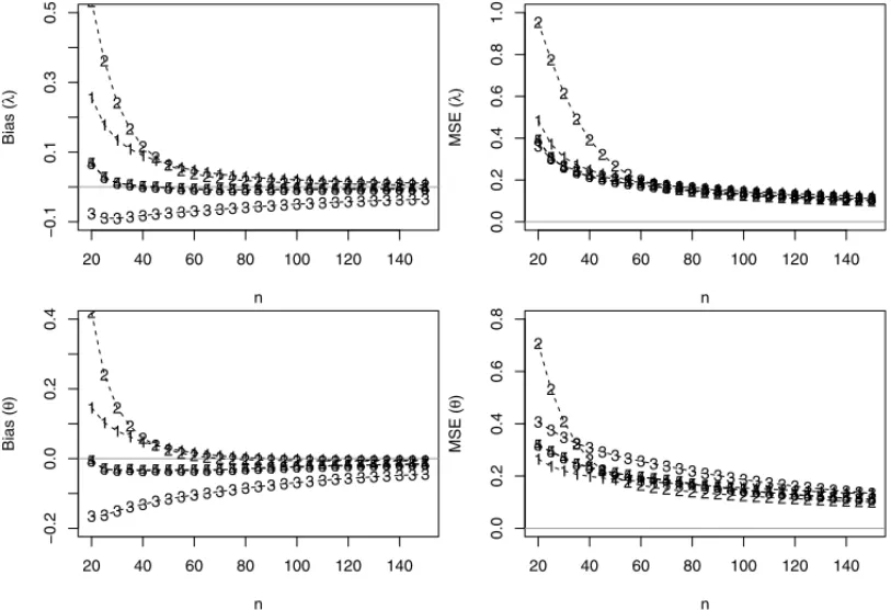
From Figure 1, the PCE, LSE, WLSE and CME estimators show a high proportion of failure in the numerical procedures. As the above estimators result in rate of failures, therefore we discarded these estimators from our simulation study. Figure 2 shows the Bias, MSEs for the es-timates ofλandθobtained by using different estimation methods for 500,000 simulated samples and considering different values ofn. We have presented results only forλ=1 andθ=0.8 due to space constraint. But the results are similar for other choices forλandθ.
1
1 1
1 1
1 1 1 1 11 1 1 1 1 1 1 1 1 1 1 1 1 1 1 1 1
20 40 60 80 100 120 140
−0.1 0.1 0.3 0.5 n Bias ( λ ) 2 2 2 2 2 2
2 2 2 2 22 2 2 2 2 2 2 2 2 2 2 2 2 2 2 2
3 3 3 3 3 3 3 3 3 3 3 33 3 3 3 3 3 3 3 3 3 3 3 33 3 4
4 4 4 4 4 4 4 4 4 4 4 4 4 4 4 4 4 4 4 4 4 4 4 4 4 4 5
5 5 5 5 5 5 5 5 5 5 5 5 5 5 5 5 5 5 5 5 5 5 5 5 5 5
1 1
1 1
1 1 1 1 1 11 1 1 1 1 1 1 1 1 1 1 1 1 1 1 1 1
20 40 60 80 100 120 140
0.0 0.2 0.4 0.6 0.8 1.0 n MSE ( λ ) 2 2 2 2 2 2 2 2 2 2
2 2 2 2 2 2 2 2 2 2 2 2 2 2 2 2 2 3
3 3
3 3 3 3 3 3 33 3 3 3 3 3 3 3 3 3 3 3 3 3 3 3 3 4
4 4 4 4 4
4 4 4 4 4 4 4 4 4 4 4 4 4 44 4 4 4 4 4 4 5
5 5 5 5 5
5 5 5 5 5 5 5 5 5 5 5 5 5 55 5 5 5 5 5 5
1 1
1 1
1 1 1 1 1 11 1 1 1 1 1 1 1 1 1 1 1 1 1 1 1 1
20 40 60 80 100 120 140
−0.2 0.0 0.2 0.4 n Bias ( θ ) 2 2 2 2 2 2
2 2 2 2 2 2 2 2 2 2 2 2 2 2 2 2 2 2 2 2 2
3 3 33 3 3
3 3 3 3 33 3 3 3 3 3
3 3 3 3 3 3 3 3 3 3 44 4 4 4 4 4 4 4 4 4 4 4 4 4 4 4 4 4 4 4 4 4 4 4 4 4
55 5 5 5 5 5 5 5 5 5 5 5 5 5 5 5 5 5 5 5 5 5 5 5 5 5 1 1
1 1 1 1 1 1 1 1 1 1 11 1 1 1 1 1 1 1 1 1 1 1 1 1
20 40 60 80 100 120 140
0.0 0.2 0.4 0.6 0.8 n MSE ( θ ) 2 2 2 2 2 2 2
2 2 2 2 2 2 2 2 2 22 2 2 2 2 2 2 2 2 2 3
3 3
3 3 33 3 3 3 3
3 3 3 3 3 3 33 3 3 3 3 3 3 3 3 4 4
4 4 4
4 4 4 4 4 4 4 4
4 4 4 4 4 4 4 4 4 4 4 4 4 4 5 5
5 5 5
5 5 5 5 5 5 5 5
5 5 5 5 5 5 5 5 5 5 5 5 5 5
Figure 2: Bias, MSEs related from the estimates ofλandθforNsimulated samples, considering different values ofn obtained using the following estimation method 1-ME, 2-MLE, 3-MPS, 4-ADE, 5-RADE.
1 1
1 1
1 1
1 1 1 1 11 1 1 1 1 1 1 1 1 1 1 1 1 1 1 1
20 40 60 80 100 120 140
0.0 0.5 1.0 1.5 n Bias ( λ ) 2 2 2 2 2 2 2
2 2 2 2 2 2 2 2 2 2 22 2 2 2 2 2 2 2 2 3 3 3 3 3 3 3 3 3 3 3 3 3 3 3 3 3 3 3 3 3 3 3 3 3 3 3 4 4 4 4
4 4 4 4 4 4 4 4 4 4 4 4 4 4 4 4 44 4 4 4 4 4 5 5 5 5
5 5 5 5 5 5 5 5 5 5 5 5 5 5 5 5 55 5 5 5 5 5
1 1
1 1 1
1 1 1 1
1 1 1 1 1 1 1 1 1 1 1 1 1 11 1 1 1
20 40 60 80 100 120 140
0.0 0.5 1.0 1.5 2.0 n MSE ( λ ) 2 2 2 2 2 2 2 2 2
2 2 2 2 2 2 2 2 2 2 2 2 2 2 22 2 2 3
3 3 3
3 3 3 3 3 3 3 3 3 33 3 3 3 3 3 3 3 3 3 3 3 3 4
4 4 4 4 4 4
4 4 4 4 4 4 4 4 4 4 4 4 44 4 4 4 4 4 4 5
5 5 5 5 5 5
5 5 5 5 5 5 5 5 5 5 5 5 55 5 5 5 5 5 5
1 1
1 1 1 1 1
1 1 1 1 1 1 1 1 1 11 1 1 1 1 1 1 1 1 1
20 40 60 80 100 120 140
−0.2 0.0 0.2 0.4 0.6 n Bias ( θ ) 2 2 2 2 2 2
2 2 2 2 2 2 2 2 2 22 2 2 2 2 2 2 2 2 2 2 3 3 3 3 3 3 3 3 3 3 3 3 3 3 3 3 3 3 3 3 3 3 3 3 3 3 3 4
4 4 4
4 4 4 4 4 4 4 4 4 4 4 4 4 4 4 4 4 4 4 4 4 4 4 5
5 5 5 55 5 5 5 5 5 5 5 5 5 5 5 5 5 5 5 5 5 5 5 5 5
1 1
1 1 1
1 1 1 1 1 1 1 1 1 11 1 1 1 1 1 1 1 1 1 1 1
20 40 60 80 100 120 140
0.0 0.2 0.4 0.6 0.8 n MSE ( θ ) 2 2 2 2 2
2 2 2 2 2 2 22 2 2 2 2 2 2 2 2 2 2 2 2 2 2 3 3 3
3 3 3 3 3 3 3 3 3 33 3 3 3 3 3 3 3 3 3 3 3 3 3 4
4 4
4 4 4 4 44 4 4 4 4 4
4 4 4 4 4 4 4 4 4 4 4 4 4 5
5 5
5 5 5 5 55 5 5 5 5 5
5 5 5 5 5 5 5 5 5 5 5 5 5
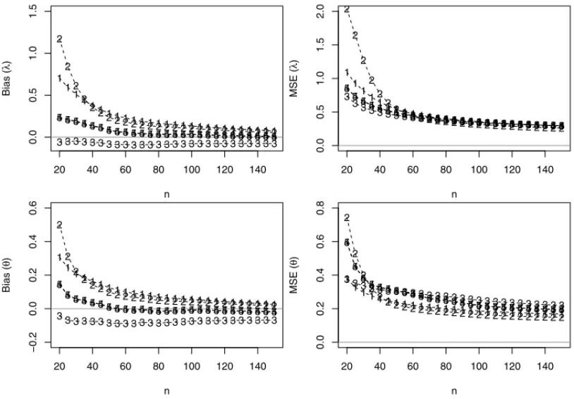
Figure 3: Bias, MSEs related from the estimates ofλandθforNsimulated samples, considering different values of n obtained using the following estimation method 1-ME, 2-MLE, 3-MPS, 4-ADE, 5-RADE.
5 APPLICATIONS
Located in southeastern Brazil, S˜ao Carlos is a city of 238,958 inhabitants. The city has an active industrial profile and high agricultural importance. Therefore, the study of the behaviour of dry and wet periods has proved to be strategic and economically significant for the regional development. From Figure 4, we observe that the city has rainy periods from October to March, and from June to August exhibit more dry periods.
Consequently, prediction of the behavior of the transition periods in rainy sessions (April, May and September) enables the agriculturists to be prepared against different problems, such as water scarcity. In this paper, we consider three real data sets related to the total monthly rainfall during April, May and September at S˜ao Carlos. The data sets (see the Appendix for more details) was obtained from the Department of Water Resources and Power agency manager of water resources of the State of S˜ao Paulo including a period from 1960 to 2014.
5.1 Initial Values
Figure 4: Average of the total monthly rainfall from January to December at S˜ao Carlos, Brazil.
any application these values are unknown. A good choice as initial values would be to use the MEs (3.6), since these estimators have closed-form expressions. However, we have shown in Section 4 that the MEs may not be computed in some cases.
Two problems can arise during the application of the MEs. First, we may have 2sx¯2>2, i.e.,
θwill be a complex number. Second 2sx¯2<1, i.e,θto be greater than 1. The first problem can
be overcome by taking the absolute value among
2−2sx¯2
, while the second can be
over-come by taking the minimum value between
2−2sx¯2
and 1. Therefore, we have chosen the modified estimator and is given by
˜
θ=min
2−2
s
¯
x
2
,1
, and λ˜ = 2 ˜
θx¯ (5.1)
where|x|is the absolute value ofx. In this caseλandθcan be computed without any problem. Note that, here we suggest the use of this estimator as initial value to be used in the iterative methods.
5.2 Discrimination Criterion Methods
the minimum values of these criteria. The Kolmogorov-Smirnov (KS) test is also considered in order to check the goodness of the fit for the models. This procedure is based on the KS statistic
Dn =supx|Fn(x)−F(x;θ , λ)|, where supxis the supremum of the set of distances,Fn(x)is
the empirical distribution function andF(x;θ , λ)is c.d.f. Under a significance level of 5% if the data comes fromF(x;θ , λ)(null hypothesis), the hypothesis is rejected if the p-value is smaller than 0.05.
For the sake of comparison, the results obtained from the BE2 distribution are compared with the Weibull, Gamma, Lognormal, Gumbel and Generalized Exponential [13] distributions and nonparametric survival function.
5.3 Results
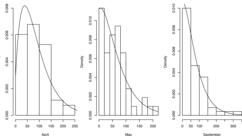
The data sets related to May and September have the occurrence of zero values, i.e., non oc-currence of precipitation. This type of data does not allow us to fit popular distributions such as Gamma, Weibull, Lognormal and Generalized Exponential distribution since they are defined only forx>0. To overcome this problem, we approximate 0.0 in the data set to 0.1. Although this is not a standard procedure, yet, without changing this results we will not be able to fit these common distributions. Nadarajah & Haghighi [20] observed that maximum likelihood estimate of the shape parameter is non-unique for the Gamma, Weibull and Generalized exponential dis-tributions if data set consists of zeros and therefore none of these three disdis-tributions can fit this kind of data set. On the other hand the BE2 distribution is defined asx≥ 0, which allow us to use the original values in the presence of zero.
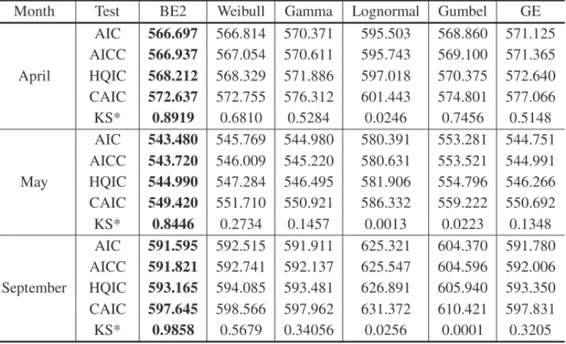
Table 1 presents the results for AIC, AICC, HQIC and CAIC criteria, for different probability distributions. In the Figure 5, we have the survival function adjusted by different distributions and non-parametric survival estimator.
Comparing the empirical survival function with the adjusted distributions it is observed that the BE2 distribution fits best among the chosen models. This result is confirmed from AIC, AICC, HQIC and CAIC criteria as the BE2 distribution has the minimum values. Considered the parametric bootstrap confidence intervals [12] in order to build the confidence intervals for the parameters of BE2 distribution using the Anderson-Darling estimates.
Table 2 displays the MLEs and 95% confidence intervals forθandλof the BE2 distribution.
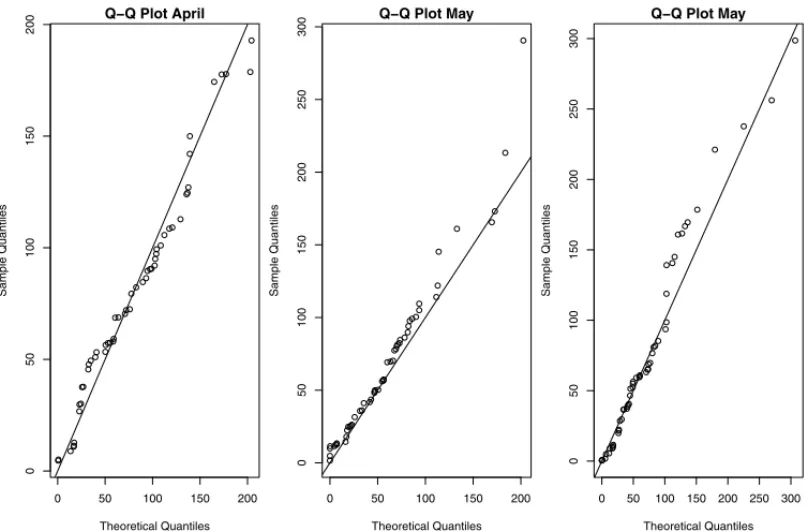
The quantile-quantile (Q-Q) plot is a graphical technique which provides an assessment of good-ness of fit. If the data set comes from the proposed distribution, the points should fall approxi-mately along the 45-degree reference line. Figures 4 and 5 display the histogram and the Q-Q plot from the proposed data set.
50 100 150 200
0.0
0.2
0.4
0.6
0.8
1.0
April
mm
S(t)
50 100 150 200
0.0
0.2
0.4
0.6
0.8
1.0
May
mm
S(t)
50 100 150 200 250 300
0.0
0.2
0.4
0.6
0.8
1.0
September
mm
S(t)
Empirical BE2 Weibull Gamma Lognormal Gumbel GE
Figure 5: Survival function adjusted by different distributions and a non-parametric method con-sidering the data sets related to the total monthly rainfall during April, May and September at S˜ao Carlos.
April
Density
0 50 100 150 200 250
0.000
0.002
0.004
0.006
0.008
May
Density
0 50 100 150 200
0.000
0.002
0.004
0.006
0.008
0.010
September
Density
0 50 100 200 300
0.000
0.002
0.004
0.006
0.008
0.010
Table 1: Results of the AIC, AICC, HQIC and CAIC criteria and the p-values of KS statistic for different probability distributions considering the data sets related to the total monthly rainfall during April, May and September at S˜ao Carlos.
Month Test BE2 Weibull Gamma Lognormal Gumbel GE
April
AIC 566.697 566.814 570.371 595.503 568.860 571.125
AICC 566.937 567.054 570.611 595.743 569.100 571.365
HQIC 568.212 568.329 571.886 597.018 570.375 572.640
CAIC 572.637 572.755 576.312 601.443 574.801 577.066
KS* 0.8919 0.6810 0.5284 0.0246 0.7456 0.5148
May
AIC 543.480 545.769 544.980 580.391 553.281 544.751
AICC 543.720 546.009 545.220 580.631 553.521 544.991
HQIC 544.990 547.284 546.495 581.906 554.796 546.266
CAIC 549.420 551.710 550.921 586.332 559.222 550.692
KS* 0.8446 0.2734 0.1457 0.0013 0.0223 0.1348
September
AIC 591.595 592.515 591.911 625.321 604.370 591.780
AICC 591.821 592.741 592.137 625.547 604.596 592.006
HQIC 593.165 594.085 593.481 626.891 605.940 593.350
CAIC 597.645 598.566 597.962 631.372 610.421 597.831
KS* 0.9858 0.5679 0.34056 0.0256 0.0001 0.3205
*p-values of KS statistic.
Table 2: MLE, 95% confidence intervals forθandλconsidering the data sets related to the total monthly rainfall during April, May and September at S˜ao Carlos.
Month ADE CI95%()
April θ 0.9297 (0.611; 0.996)
λ 0.0220 (0.016; 0.028)
May θ 0.7097 (0.200; 0.962)
λ 0.0254 (0.015; 0.030)
September θ 0.6375 (0.234; 0.955)
λ 0.0208 (0.017; 0.033)
6 CONCLUSIONS
0 50 100 150 200
0
50
100
150
200
Q−Q Plot April
Theoretical Quantiles
Sample Quantiles
0 50 100 150 200
0
50
100
150
200
250
300
Q−Q Plot May
Theoretical Quantiles
Sample Quantiles
0 50 100 150 200 250 300
0
50
100
150
200
250
300
Q−Q Plot May
Theoretical Quantiles
Sample Quantiles
Figure 7: Q-Q plot from the data sets related to the total monthly rainfall.
we have presented the simulation study results in order to identify the most efficient procedure. The simulation results show that the Anderson-Darling estimators outperform other procedures such as the maximum likelihood method for estimating the parameters of the BE2 distribution. The proposed methodology is applied in three real data sets related to the total monthly rainfall during April, May and September at S˜ao Carlos, Brazil, demonstrating that the BE2 distribution can be used as alternative to some well known distributions in weather related data.
ACKNOWLEDGEMENTS
The authors are very grateful to the Editor and the reviewers for their helpful and useful com-ments that improved the manuscript.
7 APPENDIX A – DATA SET
• April: 59.00, 102.20, 17.30, 23.00, 50.60, 27.00, 203.00, 40.90, 53.00, 177.40, 94.60, 129.40, 76.00, 93.20, 22.80, 98.80, 77.70, 204.20, 16.90, 55.10, 103.90, 34.90, 39.70, 137.70, 104.20, 117.60, 17.10, 120.80, 164.90, 50.20, 172.80, 58.50, 112.40, 24.50, 32.80, 64.00, 72.10, 139.30, 0.50, 70.90, 0.80, 82.70, 108.60, 32.30, 13.60, 25.70, 135.80, 136.80, 89.70, 139.20, 102.80, 97.30, 60.60.
19.20, 69.10, 133.00, 111.40, 25.90, 33.50, 46.80, 54.60, 43.00, 46.50, 83.60, 73.50, 18.00, 16.30, 70.00, 56.30, 70.90, 183.70, 78.20, 6.20, 86.00, 66.10, 72.80, 20.90, 17.20, 113.90, 169.60, 22.10.
• September: 26.40, 12.50, 1.00, 44.80, 0.00, 74.20, 179.50, 76.70, 269.50, 49.00, 306.80, 102.70, 73.50, 35.20, 72.70, 28.80, 49.30, 132.00, 151.50, 39.70, 136.20, 112.00, 17.70, 11.60, 225.20, 102.60, 27.10, 17.50, 6.70, 82.20, 40.70, 54.60, 115.50, 89.50, 0.00, 17.00, 127.40, 41.70, 43.10, 84.70, 102.50, 120.90, 80.10, 18.10, 5.30, 59.50, 26.80, 0.00, 34.30, 101.10, 60.30, 31.50, 60.40, 45.30, 49.50, 70.44.
RESUMO.Neste trabalho, apresentamos diferentes m´etodos de estimac¸˜ao para os
parˆame-tros da distribuic¸ ˜ao binomial-exponencial 2, tais como, estimador de m´axima
verossimilhan-c¸a, m´etodo dos momentos, m´etodo percentil, estimador de m´ınimos quadrados, m´etodo do m´aximo produto espac¸ado, estimador de Cram´er-von-Mises, estimador de Anderson-Darling
e o estimador de Anderson-Darling com cauda a direita s˜ao apresentados. Com base em um estudo de simulac¸˜ao num´erica, verificamos que o estimador de Anderson-Darling retorna
estimativas mais eficientes se comparado com os outros estimadores. Por fim, nossa proposta ´e aplicada em trˆes conjuntos de dados relacionados `a pluviosidade total mensal ao longo dos
meses de Abril, Maio e Setembro em S˜ao Carlos, Brasil.
Palavras-chave:distribuic¸˜ao exponencial-binomial 2, estimador de m´axima
verossimilhan-c¸a, estimador de Cram´er-von-Mises, estimador de Anderson-Darling.
REFERENCES
[1] M.R. Alkasasbeh & M.Z. Raqab. Estimation of the generalized logistic distribution parameters: Comparative study.Statistical Methodology,6(2009), 262–279.
[2] T.W. Anderson & D.A. Darling. Asymptotic theory of certain “goodness of fit” criteria based on stochastic processes.The Annals of Mathematical Statistics,23(2) (1952), 193–212.
[3] T.W. Anderson & D.A. Darling. A test of goodness of fit.Journal of the American Statistical Associ-ation,49(1954), 765–769.
[4] A. Asgharzadeh, H.S. Bakouch & M. Habibi. A generalized binomial exponential 2 distribution: modeling and applications to hydrologic events.Journal of Applied Statistics, (2016), 1–20. Available online:http://dx.doi.org/10.1080/02664763.2016.1254729
[5] A. Asgharzadeh, R. Rezaie & M. Abdi. Comparisons of methods of estimation for the half-logistic distribution.Selcuk Journal of Applied Mathematics, Special Issue (2011), 93–108.
[6] H.S. Bakouch, M.A. Jazi, S. Nadarajah, A. Dolati & R. Roozegar. A lifetime model with increasing failure rate.Applied Mathematical Modelling,38(2014), 5392–5406.
[8] D.D. Boos. Minimum Anderson-Darling estimation.Communications in Statistics-Theory and Meth-ods,11(1982), 2747–2774.
[9] R. Cheng & N. Amin. Estimating parameters in continuous univariate distributions with a shifted origin.Journal of the Royal Statistical Society, Series B (Methodological),45(1983), 394–403.
[10] R. Cheng & M. Stephens. A goodness-of-fit test using Moran’s statistic with estimated parameters. Biometrika, (1989), 385–392.
[11] S. Dey, T. Dey & D. Kundu. Two-parameter Rayleigh distribution: different methods of estimation. American Journal of Mathematical and Management Sciences,33(2014), 55–74.
[12] B. Efron & R.J. Tibshirani. An introduction to the bootstrap. CRC press, (1994), 1st Edition, 436 p.
[13] R.D. Gupta & D. Kundu. Generalized exponential distribution: Different method of estimations. Journal of Statistical Computation and Simulation,69(2001), 315–337.
[14] A. Henningsen & O. Toomet. maxlik: A package for maximum likelihood estimation in R. Compu-tational Statistics,26(2011), 443–458.http://dx.doi.org/10.1007/s00180-010-0217-1.
[15] J.H. Kao. Computer methods for estimating Weibull parameters in reliability studies.IRE Transac-tions on Reliability and Quality Control,13(1958), 15–22.
[16] J.H. Kao. A graphical estimation of mixed Weibull parameters in life-testing of electron tubes. Tech-nometrics,1(1959), 389–407.
[17] F. Louzada, P.L. Ramos & G.S. Perdon´a. Different estimation procedures for the parameters of the extended exponential geometric distribution for medical data. Computational and Mathematical Methods in Medicine,2016(2016). Article ID 8727951, 12 pages. doi:10.1155/2016/8727951.
[18] A. Luce ˜no. Fitting the generalized Pareto distribution to data using maximum goodness-of-fit estima-tors.Computational Statistics & Data Analysis,51(2006), 904–917.
[19] J. Mazucheli, F. Louzada & M. Ghitany. Comparison of estimation methods for the parameters of the weighted Lindley distribution.Applied Mathematics and Computation,220(2013), 463–471.
[20] S. Nadarajah & F. Haghighi. An extension of the exponential distribution. Statistics, 45(2011), 543–558.
[21] P. Ramos & F. Louzada. The generalized weighted Lindley distribution: Properties, estimation and applications.Cogent Mathematics,3(2016), 1–18.
[22] B. Ranneby. The maximum spacing method. An estimation method related to the maximum likelihood method.Scandinavian Journal of Statistics,11(1984), 93–112.
[23] G.C. Rodrigues, F. Louzada & P.L. Ramos. Poisson-exponential distribution: different methods of estimation.Journal of Applied Statistics, (2016), pp. 1–17. Available online:http://dx.doi.org/ 10.1080/02664763.2016.1268571
[24] V.K. Sharma, S.K. Singh, U. Singh & F. Merovci. The generalized inverse Lindley distribution: A new inverse statistical model for the study of upside-down bathtub data.Communications in Statistics-Theory and Methods,45(2016), 5709–5729.
[25] J.J. Swain, S. Venkatraman & J.R. Wilson. Least-squares estimation of distribution functions in John-son’s translation system.Journal of Statistical Computation and Simulation,29(1988), 271–297.