CAMILA FERREIRA AZEVEDO
RIDGE, LASSO AND BAYESIAN ADDITIVE-DOMINANCE GENOMIC MODELS AND NEW ESTIMATORS FOR THE EXPERIMENTAL
ACCURACY OF GENOME SELECTION
Tese apresentada à Universidade Federal de Viçosa, como parte das exigências do Programa de Pós-Graduação em Estatística Aplicada e Biometria, para obtenção do título de Doctor Scientiae.
VIÇOSA
ii
Ao meu pai, Sergio; por ter dedicado a
iii
AGRADECIMENTOS
A Deus por me amparar nos momentos difíceis, dar força interior para superar as dificuldades e indicar o caminho nas horas incertas.
A Universidade Federal de Viçosa e ao Programa de Pós-Graduação em Estatística Aplicada e Biometria, por proporcionar a realização de um curso de excelência.
Aos meus pais, Marilia e Sergio, pelo amor incondicional, pelos ensinamentos, pela dedicação e confiança.
À minha irmã, Lorena, pelas palavras de carinho e de incentivo e por sempre estar ao meu lado.
Ao meu noivo Vitor, pela paciência, companheirismo, amor, carinho e incentivo em todos os momentos.
Às minhas queridas avós Arlene e Marilza, por todas as orações. À minha querida família, por me apoiar em todos os momentos.
Aos meus amigos do PPESTBIO, em especial a Laís e a Gabi, pelos ótimos momentos, pelas trocas de experiência, pelas palavras de conforto e de motivação.
Aos meus amigos da Matemática, em especial Amanda, Izabela, Victor e Marcelo, pela valiosa amizade, por sempre se fazerem presentes e por torcerem sempre por mim.
Ao Doutor e orientador Marcos Deon Vilela de Resende, pelos ensinamentos, confiança, dedicação, por contribuir para o meu crescimento profissional e por ser também um exemplo de pesquisador admirável e generoso.
Aos Doutores e coorientadores Fabyano Fonseca e Silva e Moyses Nascimento, pelos saberes transmitido, pela confiança, disponibilidade, incentivo e generosidade.
Ao Doutor José Marcelo Soriano Viana pela disponibilidade e pela imprescindível ajuda na execução deste trabalho.
iv
Aos membros da banca examinadora, Prof. Doutor Fabyano Fonseca e Silva, Prof. Doutor José Marcelo Soriano Viana, Prof. Doutor Júlio Sílvio de Sousa Bueno Filho, Prof. Doutor Marcos Deon Vilela de Resende, Prof. Doutor Moyses Nascimento, pela disponibilidade e pelas valiosas sugestões para o enriquecimento deste trabalho.
Aos professores do Programa de Pós-Graduação em Estatística Aplicada e Biometria e atuais colegas de trabalho, por contribuírem para minha formação acadêmica, por me auxiliarem e me conduzirem à prática docente, em especial aos Professores e amigos Ana Carolina Campana Nascimento, Moyses Nascimento, Paulo Roberto Cecon e Antonio Policarpo Souza Carneiro.
As secretárias e amigas do Departamento de Estatística, Anita e Carla, pela amizade, incentivo e carinho.
A FAPEMIG, pela concessão da bolsa de estudos.
v BIOGRAFIA
CAMILA FERREIRA AZEVEDO, filha de Marilia Assis Ferreira Azevedo e de Sergio de Rezende Azevedo, nasceu em Bom Jesus do Itabapoana, Rio de Janeiro, em 15 de abril de 1988.
Em maio de 2006, ingressou no curso de Licenciatura em Matemática na Universidade Federal de Viçosa, Viçosa-MG, graduando-se em julho de 2010. Em agosto do mesmo ano, iniciou o curso de Mestrado no Programa de Pós-Graduação em Estatística Aplicada e Biometria na Universidade Federal de Viçosa, submetendo-se à defesa de dissertação em 26 de julho de 2012.
vi
SUMÁRIO
RESUMO ... VIII ABSTRACT ... X
GENERAL INTRODUCTION ... 1
CHAPTER 1 ... 4
LITERATUREREVISION ... 4
1. Statistical Methods for Additive-Dominance Models... 4
1.1.2.1. Normal distribution ... 6
1.1.2.2. Student's t-distribution ... 7
1.1.2.3. Double Exponential distribution... 9
1.1.2.4. Scaled inverse chi-square distribution ... 10
2. References ... 25
CHAPTER 2 ... 31
RIDGE,LASSOANDBAYESIANADDITIVE-DOMINANCEGENOMIC MODELS ... 31
ABSTRACT ... 31
1. Background ... 32
2. Methods ... 35
3. Results ... 51
1.1. Statistical concepts ... 4
1.1.1. Shrinkage ... 5
1.1.2. Probability distributions ... 6
1.1.3. Additive-Dominance Model for the REML/G-BLUP method .. 11
1.1.4. Bayesian Ridge Regression (BRR) Method ... 14
1.1.5. Ridge Regression with heterogeneity of variances (RR-HET) .. 15
1.1.6. BayesA and BayesB methods ... 15
1.1.7. BayesA method ... 16
1.1.8. BayesB method ... 19
1.1.9. LASSO method ... 20
1.1.10. BLASSO method ... 21
1.1.11. IBLASSO method ... 23
2.1. Simulated datasets ... 35
2.2. Scenarios ... 37
2.3. Statistical Methods for Additive-Dominance Models... 38
2.3.1. Additive-Dominance Model for the REML/G-BLUP method .. 38
2.3.2. Bayesian Ridge Regression (BRR) Method ... 40
2.3.3. BayesA and BayesB methods ... 40
2.3.4. BayesA*B* or IBLASSOt method ... 43
2.3.5. BLASSO and IBLASSO Methods ... 46
2.3.6. Ridge Regression with heterogeneity of variances (RR-HET) .. 47
2.4. Fitting Models ... 47
2.5. Methods for Computing Parametric Accuracies ... 49
vii
4. Discussion ... 59
5. Conclusions ... 64
6. References ... 64
CHAPTER 3 ... 81
REGULARIZEDANDHYBRIDESTIMATORSFORTHEEXPERIMENTAL ACCURACYOFGENOMESELECTION ... 81
ABSTRACT ... 81
1. Introduction ... 83
2. Methods ... 85
3. Results and Discussion ... 94
4. References ... 97
APPENDIX 1 ... 108
Deterministic formula for the predictive ability ryyˆ , molecular heritability 2 M h and accuracy rggˆ of GWS... 108
3.1. Comparison of Methods ... 51
3.2. Partition of accuracy due to the three quantitative genetics information 56 2.1. Simulated datasets ... 85
2.2. Scenarios ... 87
2.3. Traditional accuracy estimator (TE) ... 88
2.4. Regularized estimator (RE) ... 90
2.5. Hybrid estimator (HE)... 91
2.6. Parametric Accuracy ... 92
2.7. Supervised RR-BLUP ... 92
viii RESUMO
AZEVEDO, Camila Ferreira, D.Sc., Universidade Federal de Viçosa, outubro de 2015. Modelos genômicos aditivo-dominante via abordagem Ridge, Lasso e Bayesiana e novos estimadores para a acurácia experimental da Seleção Genômica. Orientador: Marcos Deon Vilela de Resende. Coorientadores: Fabyano Fonseca e Silva e Moyses Nascimento.
ix
x ABSTRACT
AZEVEDO, Camila Ferreira, D.Sc., Universidade Federal de Viçosa, October, 2015. Ridge, Lasso and Bayesian additive-dominance genomic models and new estimators for the experimental accuracy of Genome Selection. Adviser: Marcos Deon Vilela de Resende. Co-advisers: Fabyano Fonseca and Silva and Moyses Nascimento.
xi
1
GENERAL INTRODUCTION
Recently there was advancement in molecular genetics which promoted an rapid evolution of sequencing and genotyping technologies. The molecular genetics can benefit the plant and animal breeding in terms of the identification of genetically superior individuals by using directly the information from DNA. The use of molecular markers allows an increase in selection efficiency and speed in obtaining desirable genetic gains.
The single nucleotide polymorphisms (SNPs) genetic markers are the most used in genomic prediction, due to its low mutation rate, codominance and abundance. Due to the availability of high density of SNPs markers in the genome, Meuwissen et al. (2001) developed the genome-wide selection (GWS), as an approach to accelerating the breeding cycle. The GWS consists in an analysis of a large number of markers widely distributed in the genome, capturing the genes affecting quantitative traits of interest.
It is possible to assume that some markers are in linkage disequilibrium (LD) with quantitative trait loci (QTL), enabling, together with phenotypic data, its direct use in the estimation of the genetic value of individuals subject to selection, including individuals who have not yet been phenotyped. However, the number of markers is generally much larger than the number of genotyped and phenotyped individuals and that markers are highly correlated, which requires appropriate statistical methods that enable estimability and regularization properties (Gianola et al., 2003).
2
and validation populations. Reports on these topics are common for additive genetic models but not for additive-dominance models. However, it is known that dominance estimation is essential specially for vegetative propagated species (Denis and Bouvet, 2013) and crossed populations, where the mating allocation including both additive and dominance is an effective way of increasing genetic gain capitalizing on heterosis (Toro and Varona, 2010; Wellmann and Bennewitz, 2012). Additive-dominance models are able to capture both effects, allowing effective selection for parents, crosses and for clones. This allows taking full advantage of genomic selection in perennials and asexually propagated crops and also in crossed animals. In addition, the inclusion of dominance in the prediction model may improve the accuracy of genomic prediction when dominance effects are present (Wang et al., 2014; Hu et al., 2014; Su et al., 2012).
3
In addition, the evaluation of the methods applied to genomic selection consist in one of the main lines of research in this area and the main measure for evaluating the efficiency of the prediction of genomic breeding values is the experimental accuracy (after obtaining data). However, traditional accuracy estimators (Legarra et al., 2008; Hayes et al., 2009a) have some practical and theoretical inconsistencies, which lead erroneous conclusions in some circumstances. Estaghvirou et al. (2013) carried out a comparative study among alternative accuracy estimators for GWS, but such estimators only differed from the estimator of Legarra et al. (2008) and Hayes et al. (2009a) in the different ways of estimating the trait heritability. In fact, to date, there are no proposed estimators for the experimental accuracy of genomic selection, but only for the expected (before obtaining data) accuracy (Daetwyler et al., 2008; 2010; Resende, 2008; Goddard, 2009; Goddard et al., 2011; Hayes et al. 2009b).
4 CHAPTER 1
LITERATURE REVISION
1. Statistical Methods for Additive-Dominance Models
Statistical methods for genomic selection can be divided in three groups: explicit regression methods (Ridge, Bayesian and Lasso regression, etc), implicit regression methods (Kernel, Reproducing Kernel Hilbert Spaces - RKHS, Neural Networks, etc), dimensionality reduction methods (principal components regression, partial least square regression, independent components regression, etc). The explicit regression methods encompassing the penalization and Bayesian methods such as ridge regression (RR), Bayesian RR (BayesRR), Bayesian LASSO (BLASSO) and BayesA and B of Meuwissen et al. (2001). These are the main approaches being applied in practical genomic selection (De los Campos et al, 2012; Resende Jr., et al. 2012; Gianola, 2013; Lehermeier et al., 2013). The Bayesian methods are Bayesian linear regression that differs in the priors adopted while sharing the same model (Gianola, 2013). Daetwyler et al. (2012) recommended comparing accuracy and bias of new methods to results from genomic best linear prediction and a variable selection approach with specific variance components for each locus such as BayesB, because, together, these methods are appropriate for a range of genetic architectures.
1.1. Statistical concepts
5 1.1.1. Shrinkage
The shrinkage methods consist in constraints on the size of coefficient estimates, or equivalently, shrinks the coefficient estimates towards zero relative to the least squares estimates. These methods leads to an economy in the degrees of freedom (regularization property) and leads to stable estimates, allowing for the estimability of the parameters in the n >> N case, where n is the covariables numbers and N is the observations number, and when there is multicollinearity among the variables. Thus, this property is very important to high dimensionality case. The shrinkage effect considers the sample size and variations of random and residual effects.
Among the methodologies applied to genomic selection, the penalization and Bayesian methods are also called shrinkage methods. The shrinkage is implicit in Bayesian Inference and the degree of shrinkage is controlled by the assumed prior distribution to markers effects. The bayesian prediction of genomic breeding values (obtained by SNPs effects - m) is based in the bayesian estimation, which is equivalent the conditional mean of the genetic value given the individuals genotype at each QTL (Resende et al., 2012). Thus, based on markers and considering each QTL separately, the markers effects (m) are given by the conditional expectation
ˆ
(
)
m E m | y
. The appropriate bayesian estimator is obtained by Bayes' theorem and is given by:( | ) ( )
ˆ ( )
( | ) ( )
m
m
R
R
mf y m f m dm m E m | y
f y m f m dm
,6
dependent of assumed prior distribution to the markers effects (or putative QTLs) and consequently the degree of shrinkage ascribed.
The presence of QTL is analyzed in many positions, as there are thousands SNPs widely distributed in the genome (Goddard and Hayes, 2007), but it is known that not all markers are in linkage disequilibrium with the QTL. Thus, the ideal prior distribution f m( ) should have a high density in f(0), produced by shrinkage of each prior distribution. Therefore, the shrinkage leads many effects equal to zero and consequently a more favorable statistical condition, i. e., more individuals (N) to estimate less markers effects (n) (the lower the ratio n
N , the better estimation
process). In addition, learning about genetic architecture without contamination from effects of the prior does not take place whenever N ≪ n (Gianola, 2013).
1.1.2. Probability distributions
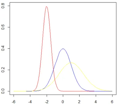
1.1.2.1. Normal distribution
Normal distributions are extremely important in statistics, since the most known statistical procedures assume that the continuous random variables follows this distribution. The normal probability density function is:
2 2 ( )
2 1
( )
2 x
f x e
,
x
where the parameter of location
is the mean or expectation of the distribution, the parameter of scale is the standard deviation and 2is the variance.
7
in yellow has a mean of 1 and a standard deviation of 2.5. These as well as all other normal distributions are symmetric with relatively more values at the center of the distribution and tails less dense.
Figure 1. Normal distributions differing in the mean (-2, 0 and 1 – red, blue and yellow, respectively) and
standard deviation (0.5, 1 and 1.5 – red, blue and yellow, respectively).
1.1.2.2. Student's t-distribution
The Student's t-distribution (or t-distribution) is also a member of a family of continuous probability distributions that arises when estimating the mean of a normally distributed population in situations where the sample size is small and population standard deviation is unknown. However, the larger the sample, the more the distribution resembles a normal distribution. Student's t-distribution has the probability density function given by:
1
2 2
1 2
( ) 1
2
v v
x f x
v v
v
8
where v is the number of degrees of freedom and
is the gamma function. The mean of t random variable is 0 for v0 and variance is2 v
v for v2 or ∞ for
1 v 2.
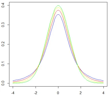
The Figure 2 shows t distributions with 4 (blue), 6 (red), and 12 (yellow) degrees of freedom and the standard normal distribution (green). It can be seen that as the number of degrees of freedom increases the tails of the distributions become heavier. Notice also, that the normal distribution has relatively more scores in the center of the distribution and the t distribution has relatively more in the tails. The t-distribution is therefore leptokurtic, meaning that it is more prone to producing values that fall far from its mean and more extreme values. That is, most effects are close to zero, but some extremely big. The t-distribution approaches the normal distribution as the degrees of freedom increases.
Figure 2. The t-distributions with 2, 4, and 10 (blue, red and yellow, respectively) degrees of freedom and the
9
1.1.2.3. Double Exponential distribution
The double exponential distribution is a continuous probability distribution, also sometimes called the Laplace distribution. The double exponential distribution can be thought of as two exponential distributions (with an additional location parameter) spliced together back-to-back. The general formula for the probability density function of the double exponential distribution is:
| | 1 ( )
2 x
f x e
,
x
where
is a location parameter and 0 is a scale parameter. The mean of random variable is
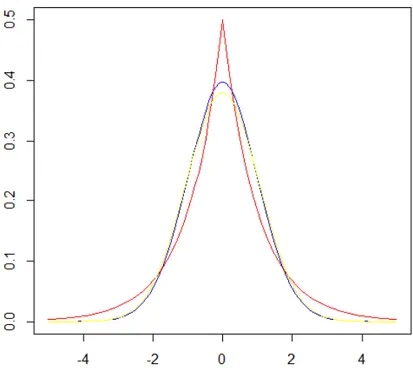
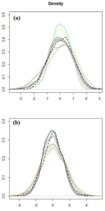
and variance is 2~2.Figure 3. Densities of double exponential (red), normal (yellow) and t (blue) distributions, all with zero means
and variances equal to unity.
10
higher mass density at zero and thicker tails, meaning that it is more prone to producing values closer to zero, and the more extreme values than the normal distribution. The double exponential distribution has a higher density than the t distribution.
1.1.2.4. Scaled inverse chi-square distribution
The scaled inverse chi-squared distribution is the distribution for x 12 y
,
being
y
2 is a sample mean of the squares of ν independent normal random variables that have mean 0 and inverse variance 22 1
S
. The distribution is therefore parametrized by the two quantities and 2
S , referred to as the number of chi-squared degrees of freedom and the scaling parameter, respectively. The probability density function of the scaled inverse chi-squared distribution is given by:
2 2 2 2 1 2 2 ( ) 2 v vS x v v S e f x v x
, x0.
The mean of distribution is
2
2 vS
v for v2 and the variance of distribution is
2 4
2
( 2)( 4) v S
11
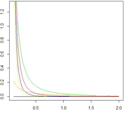
Figure 4. The scaled inverse chi-squared distributions with 0, 0.05, 2, 4, 6, and 8 degrees of freedom and all with
scale parameter equal to 0.0429.
The Figure 4 shows scaled inverse chi-squared distributions with 0 (black), 0.05 (orange), 2 (green), 4 (red), 6 (blue), and 8 (yellow) degrees of freedom (
v
) and all with scale parameter (S
2) equal to 0.0429. As the number of degrees of freedom approaches zero (orange and black curve) the scaled inverted chi-square distribution becomes approximately equivalent to uniform distribution. However, when the numbers of degrees of freedom deviates from 0, for example 2 (green curve), describe a heavy-tailed distribution. And as the number of degrees of freedom increases the distribution is replaced by a lower density tails.1.1.3. Additive-Dominance Model for the REML/G-BLUP method A mixed linear model for individual additive breeding values (
u
a) and12
a d
y Xb Zu
Zu
e
,where
y
(N × 1, N is number of phenotype and genotype individuals) is a vector of phenotypic observations or corrected phenotypes vector; b (N × 1) is a vector of fixed effects (when using corrected phenotypes is reduced to a unit vector); e( N × 1) is the random error vector, 2~ 0,I e)
e N( σ being 2 e
σ is the error variance ;
X
(N × p,p is number of fixed effects) and
Z
(N × N) are the incidence matrices for b,u
aand
u
d, respectively. The variance structure given byu N( G
a~
0,
aσ
u2a)
, 2~
0,
)
d d ud
u N( G
σ
, ( u2a
σ
is the additive variance, u2d
σ
is the dominance variance,G
aand
G
d (N × N) are the genomic relationship matrices for additive and dominance effects.).So mixed model equations to predict
u
a andu
d through the G-BLUP method is equivalent to:2 1 2 2 1 2
' ' ' ˆ
'y ˆ ' ' ' ' ˆ ' ' ' ' e a a a d e d d
X X X Z X Z
b X
Z X Z Z G Z Z u Z y
u Z y
Z X Z Z Z Z G
(1)
Thus, the genomic breeding value (GBV) of the individual j ( j = 1, … , N ) is given
by
1 1
ˆ ˆ n ˆ n ˆ
j i ij aj ij dj i i
GBV y z u z u
.An equivalent model (Goddard et al., 2010) at marker level is given by
a d
13 .
a a
2 2
a ma ma
d d
2 2
d md md
u = Wm ;
Var(Wm )= WIσ W' =WW'σ ν u = Sm ;
Var(Sm )= SIσ S' = SS'σ
W (N × n, n is number of SNPs markers) and S (N × n) are, respectively, the incidence matrices for the vectors of additive (
m
a ) and dominance (m
d) marker genetic effects. The variance components associated to these effects are m2a
σ
and2 md
σ
, respectively. The quantitym
a in one locus is the allele substitution effect givenby
m
ai
ia
i(
q
ip d
i)
i ( i = 1 ,…, n ), where pi and qi are allelic frequenciesand
a
i andd
i are the genotypic values of the homozygote and heterozygote, respectively, at the locus i. By its turn, the quantitym
d can be directly defined asdi i
m = d
. The method admits the assumption that the effects of markers are considered random, normally distributed and homogeneous variance.The matrices W and S are based on the values 0, 1 and 2 for the number of one the alleles at the i marker locus (putative QTL) in a diploid individual. Several parameterizations are available and the one that matches well with the classical quantitative genetics theory (Falconer and Mackay, 1996) is as follows (Van Raden, 2008; Da et al., 2014; Vitezica, 2013).
14
2 2
a a a ma
G σ =Var(Wm )=WW'σ , which leads to G = WW (a '/ σ σ )a2/ ma2
1
'/ 2p 1
n
i i
i=
= WW
[ ( p )], since 2 21
2p 1
n
a i i ma i=
σ = [ (
p )]σ . The covariance matrix forthe dominance effects is given by Gdσ =Var(Sm )= SS'σd2 d md2 . So
2 2 2
1
´/ / '/ 2p 1
n
d d md i i i=
G = SS (σ σ )= SS
[ ( p )] , since 2 2 21
2p 1
n
d i i md i=
σ =
[ ( p )] σ . Thecorrect parameterization in W and S is as follows, according to marker genotypes in a locus i.
If MM, then 2 2 2
If Mm, then 1 2 (2)
If mm, then 0 2 2
p q
W p q p
p p 2 2
If MM, then 0 2
If Mm, then 1 2 (3)
If mm, then 0 2
q S pq p
The G-BLUP method retains all the covariables (SNPs markers) leading to complex models. Thus, produces good results for the case in which it has many markers with small effect.
1.1.4. Bayesian Ridge Regression (BRR) Method
15
(additive and dominance effects) close to zero but not zero, since the infinitesimal model assumes loci with many small effects. BRR is expected to produce similar results as the G-BLUP and RR-BLUP.
1.1.5. Ridge Regression with heterogeneity of variances (RR-HET) A additive-dominance Ridge Regression (RR-BLUP) method can also be implemented considering the heterogeneity of variances between markers, called RR-HET. By this modification, the shrinkage is no longer homogeneous and becomes specific in accordance with the effect size and variance of the marker. The matrices with specific variances for each marker, Dadiag(
a21, a22,...,
an2 ) and2 2 2 1 2
( , ,..., )
d d d dn
D diag
, the elements
ai2 and
di2 can be obtained through Bayesian methods. The additive and dominance genetic variance of each marker locus is, simply, given by
mai2
ai2 and
mdi2
di2 (with i1, 2,...,n), respectively. Therefore, for additive and dominance genetic variance, using the relationships2 2
1
2p 1
n
a i i mai i=
σ =
( p ) σ and 2 2 21
2p 1
n
d i i mdi i=
σ = [
( p )] σ , we have2 2
1
2p 1
n
a i i ai i=
σ =
( p )
and 2 2 21
2p 1
n
d i i di i=
σ = [
( p )]
.1.1.6. BayesA and BayesB methods
16
to values near 0 (BayesA) or 0 (BayesB) and the estimated effects are dictated by the prior distributions the QTLs effects.
1.1.7. BayesA method
Meuwissen et al. (2001) presented a methodology for estimating model parameters, in which different components of variance are assigned to each segment (SNP marker) considered in the analysis. The BayesA assume few genes of large effects and many genes of small effect, in other words, specific shrinkage for each marker. This is expected to produce similar results as the RR-HET.
The BayesA method assume the conditional distribution of each marker effect (given its variance) to follow a normal distribution, i.e, m |ai σmai2 ~N( σ )0, 2mai . The variances of the marker effects are assumed to be a scaled inverse chi-square distribution with v degrees of freedom and scale parameter m2
a
S
, i.e,2 2
~ 2
mai ma ma
σ χ ( ,S )
. This implies that a larger number of markers presents small effects and a small number of markers presents big effects. Thus, the main advantage of using the scaled inverse chi-square distribution as prior for the variance components is, that when the data have normal distribution, a posterior distribution is also a scaled inverse chi-square distribution.
The use of a mixture of normal (for the effects) and scaled inverse chi-square (for variances) distributions leads to univariate t-distribution of the marker effects with mean zero (Sorensen and Gianola 2002), as follows:
2
( 1) 2
2 2 2 2
( ,S )= 0, 2 (1 ai ) ma
ai ma ma mai ma ma mai 2
ma ma R
m
p m | v N( σ )χ ( ,S )dσ
S
,~ 0,
2 2
ai ma ma ma ma
17
Gianola et al. (2009) proved that fitting a variance by locus in this way is equivalent to postulating t distribution for all loci. Thus, the identification of relevant marker effects is more likely in t-BayesA model than in normal-RR-BLUP model. The distributions used in the construction of the joint posterior density allow the use of the Gibbs sampler (Geman and Geman, 1984) to generate samples from the joint a posteriori density (and therefore, the marginal distribution of interest). At the end of the MCMC (Markov Chain Monte Carlo) process, estimates of the effects of each marker are obtained, and therefore the estimates of genomic values of each
individual are
1 1
ˆ ˆ n ˆ n ˆ
j j ij ai ij di i i
GBV y w m s m
( j = 1 ,…N).The m2
a
S
parameter can be calculated from the additive variance according toHabier et al. (2011). Then, for the additive marker genetic effects we have
2 2 ( ) 2 ma ma mai ma s v E v
and
2
2 ( ma)( ma 2)
ma ma E v S v
. The expectation E(
mai2 ) is equivalentto
2 2
1
( )
2 (1 )
a mai n i i i E p p
, where2 a
σ is the additive genetic variance of the trait
and pi is the frequency of marker allele i. As result we get
2 2
1
( 2)
( )
2 (1 )
a ma mai n ma i i i E p p
.18
equal or lower than 4 turn the a priori distribution into a flat and non-informative one.
For the residual effects we have e|σ N( σ )e2~ 0, e2 and 2~ 2 e
2 e e e
σ S χ . Also
2 2 ( ) 2 e e e e s v E v and 2
2 ( e)( e 2)
e e E v S v
. The expectation 2
e
E(σ ) is equivalent to
2 2 e e
E(σ ) σ . So, 2 2( 2) 2 (4.2 2) 4.2
e
e e e
e
v
S σ σ
v
, where σe2 is a prioi value of σe2.
Zeng et al. (2013) used v equal 4 for both genetic and environmental effects and the true simulated values for E(σ )e2 and E(σ )ma2 .
For dominance effects at the intra-population level, the distributions are similar as described for additive effects. Then:
2 2
~ 0,
di mdi mdi
m |σ N( σ ) for the marker dominance effects;
2 2
~ 2
mdi md md
σ χ ( ,S )
for the marker dominance variance;
being the marginal the prior distribution for marker dominance effects given by
~ 0,
2 2
di md md md md
m |
,S t(
,S )
.Additive and dominance variances are given by 2 2
1
2p 1
n
a i i ai i=
σ =
( p ) m and2 2 2
1
2p 1
n
d i i di i=
σ =
[ ( p )] m , respectively, according to parameterizations in W and S.19 1.1.8. BayesB method
The problem in the BayesA method is the fact that the variances distribution of haploid effects does not exhibit a mass density at 0. This feature would be of interest to this distribution, since most of the segments have no genetic variance (do not present segregation). This assumption leads to a more favorable statistical condition n
N . BayesB has the same assumptions of BayesA for a fraction of
SNPs and assumes that (1) of the SNPs have no effect, where is adopted
subjectively (or by BayesCpi). It uses a priori density of QTLs effects with mass density in 2 0
i
ma
(and 2 0i
md
) with probability and σmai2 ~χ ( ,S )2 ma ma2
(and
2 2
~ 2
mdi md md
σ χ ( ,S )
) with probability (1).
In this case, the prior distributions for the additive and dominant marker effects, respectively, are given by:
2 2 2
, ~(1-I ) 0, 0 I 0, )
ai mai ai mai ai mai
m |
σ N( σ ) N( σ2 2 2
, ~(1-I ) 0, 0 I 0, )
di mdi di mdi di mdi
m |
σ N( σ ) N( σwhere the indicator variable I (
I =
ai(0,1)
andI =
di(0,1)
), so the distributions of1
(
...
)
a a an
I = I
I
andI = I
d(
d1...
I
dn)
are binomial with a probability . If 1, we have BayesA.In principle it is possible to construct a Gibbs sampler for this approach, but in doing so the Markov chain does not visit all the necessary sample space, since the marginal posterior distribution of 2
i
ma
(and 2 i
md
) do not have the form of a known
20
bringing a distribution from which there is no direct sampling. The full conditional distributions for the parameters of the BayesB model were presented in details by Zeng et al. (2013).
1.1.9. LASSO method
The Bayesian regression can be used in situations where there are more markers (covariate) than observations, once the a priori distributions impose the regularization in the model fitting in a way of shortening the regression coefficients (shrinkage). An interesting way to impose this shortening is by LASSO regression (Least Absolute Shrinkage and Selection Operator, Tibshirani, 1996), which combines variable selection (model interpretability) and regularization via shrikaging of the regression coefficients. In general, this consists in obtaining estimates of regression coefficients (2) by solving the following optimization problem:
1 1 1 1
1 1
min{[y (1 )]'[y (1 )]
| | | |}
n n n n
i ai i di i ai i di
i i i i
n n
a ai d di
i i
w m s m w m s m
m m
where
1 1
| |, | |
n n ai di i i
m m
are the sum of the absolute values of the regressioncoefficients,
a and
d are parameters that controls the strength of the smoothing, so that when
a
0
(or
d
0
) there is no regularization. The LASSO solution allows to N1 non-zero regression coefficients, where N is the number of individuals.21
markers). Thus, as
approaches zero the solution converges to the method of least squares (no selection and unstable predictive covariates). While high values of
greatly reduce the values of the regression coefficients. Thus, for the optimally calculation of
, Usai et al. (2009) proposed an algorithm based in cross-validation, which is called minimum angle regression (LARS).1.1.10.BLASSO method
The Bayesian version of the LASSO regression (BLASSO - Park and Casella, 2008) for genomic selection was designed by De Los Campos et al. (2009). The BLASSO includes a common variance term to model both terms, the residuals and genetic effects of the markers. Therefore, using the same model equation used previously for the estimation of the markers effects, we have:
2 2
|
~
(0, I
)
e
MVN
| | 2
| , ~
2
amai
a ai a i m e
| | 2 | , ~ 2dmdi
d di d i m e
,where MNV represents a multivariate normal distribution,
is the “sharpness” parameter and the 2prior distribution consists of a scaled inverse chi-square. The parameter
a (or
d) can be estimated from the data by MCMC methods (using anon-informative prior) and MCEM (Monte Carlo EM - does not require a priori information).
22
coefficients next to 0 and less shrinkage on regression coefficients distant from zero. Thus, posterior averages are estimated, producing very small values, but not zero as the original LASSO. Using a formulation in terms of an augmented hierarchical model, we have:
2
( ai | a) ~ N(0, Da )
p m
, p m( di|
d) ~ N(0, Dd
2)2 2 2 2 2 2 ( | ) 2 a ai a a a i p e
and2 2 2 2 2 2 ( | ) 2 d di d d d i p e
where Dadiag(
a21, a22,...,
an2 ) and Dddiag(
d21, d22,...,
dn2 ). This leads to doubleexponential distribution of the marker effects (Park and Casella, 2008), as follows: 2
2 2 2 2 1
( )= 0,
2 2 ai a m a
ai a ai ai
R
a
p m | N( σ )Exp d e
, 22 2 2 2 1
( )= 0,
2 2 di d m d
di d di ai
R
d
p m | N( σ )Exp d e
~ 0, ai a a 2m | DoubleExp
and di d ~ 0, d
2
m | DoubleExp
.
Bayesian Lasso are advantageous compared to Bayesian methods of Meuwissen et al. (2001) because it is asymptotically free of priori information, i.e., provides better learning from data (Gianola, 2013; Gianola et al., 2009). This occurs because in the hierarchical models, such as BLASSO a priori information is assigned to the hyperparameters so that the influence of this information disappears asymptotically (Resende et al., 2012).
The additive and dominance genetic variance of each marker locus is given by
mai2
ai2 2 and2 2 2 mdi di
23
and dominance genetic variance, using the relationships 2 2
1
2p 1
n
a i i ai i=
σ =
( p ) σ and2 2 2
1
2p 1
n
d i i di i=
σ = [ (
p )] σ , we have:2 2 2
1
2p 1
n
a i i ai i=
σ =
( p )
and 2 2 2 21
2p 1
n
d i i di i=
σ =
[ ( p )]
.The full conditional distributions for the parameters of the BLASSO model were presented in details by De Los Campos et al. (2009).
1.1.11.IBLASSO method
Legarra et al. (2011) proposed the improved BLASSO (IBLASSO) method, which uses two terms of variance, one for shaping the residuals and the other for shaping the genetic effects (additive and dominant) of markers. The parameters of IBLASSO is equivalent to the original LASSO of Tibshirani (1996), but the implementation is bayesian and does not assumes that the incidence matrices markers (W and S) are standardized.
Using a formulation in terms of an augmented hierarchical model including the extra variance components
ai2 and
di2 associated with each marker locus, we have:2 2
|
~
(0, I
)
e
MVN
( ai | a) ~ N(0, D )a
p m
, p m( di|
d) ~ N(0, D )d2 2 2 2 2 2 ( | ) 2 a ai a a a i p e
and24
where Dadiag(
a21, a22,...,
an2 ), Dddiag(
d21, d22,...,
dn2 ) and the 2 priordistribution consists of a scaled inverse chi-square. This leads to double exponential distribution of the marker effects (Legarra et al., 2011), as follows:
2 | |
2 2 2 2
( )= 0,
2 2
a ai m
a a
ai a ai ai
R
p m | N( )Exp d e
,2 | |
2 2 2 2
( )= 0,
2 2
d di m
d d
di d di di
R
p m | N( )Exp d e
, 1 ~ 0, ai a a 2m | DoubleExp
and
1
~ 0,
di d
d 2
m | DoubleExp
.
The additive and dominance genetic variance of each marker locus is, simply, given by
mai2
ai2 and
mdi2
di2 (with i1, 2,...,n), respectively. Therefore, additiveand dominance genetic variance, using the relationships 2 2
1
2p 1
n
a i i mai i=
σ =
( p ) σ and2 2 2
1
2p 1
n
d i i mdi i=
σ = [
( p )] σ , we have:2 2
1
2p 1
n
a i i ai i=
σ =
( p )
and 2 2 21
2p 1
n
d i i di i=
σ = [
( p )]
.25
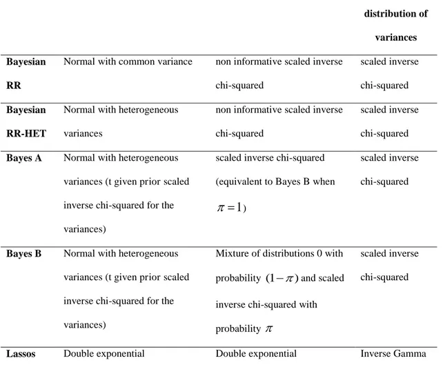
Table 1. Distributions of genetic effects on RR-BLUP, Bayes and Lasso methods. (Resende et al., 2012).
Method Prior distribution of effects Prior distribution of variances Posterior
distribution of
variances
Bayesian
RR
Normal with common variance non informative scaled inverse chi-squared
scaled inverse chi-squared
Bayesian
RR-HET
Normal with heterogeneous variances
non informative scaled inverse chi-squared
scaled inverse chi-squared
Bayes A Normal with heterogeneous variances (t given prior scaled inverse chi-squared for the variances)
scaled inverse chi-squared (equivalent to Bayes B when
1
)scaled inverse chi-squared
Bayes B Normal with heterogeneous variances (t given prior scaled inverse chi-squared for the variances)
Mixture of distributions 0 with probability (1)and scaled
inverse chi-squared with probability
scaled inverse chi-squared
Lassos Double exponential Double exponential Inverse Gamma
2. References
Da Y., Wang C., Wang S., Hu G. 2014. Mixed model methods for genomic prediction and variance component estimation of additive and dominance effects using SNP markers. PLoS One, 30,9(1):e87666.
26
Daetwyler, H. D., B. Villanueva, J. A. Woolliams. 2008. Accuracy of predicting the genetic risk of disease using a genome-wide approach. PLoS One, 3:e3395. Daetwyler, H. D., R. Pong-Wong, B. Villanueva, et al. 2010. The impact of genetic
architecture on genome-wide evaluation methods. Genetics, 185:1021–1031. De Los Campos G., Hickey J. M., Pong-Wong R., Daetwyler H. D., Callus M. P. L.
2012. Whole Genome Regression and Prediction Methods Applied to Plant and Animal Breeding. Genetics, 193:327-345.
De Los Campos G., Naya H., Gianola D., Crossa J., Legarra A., Manfredi E., Weigel K., Cotes J. M. 2009. Predicting Quantitative Traits With Regression Models for Dense Molecular Markers and Pedigree. Genetics, 182(1):375-385.
Denis M., Bouvet J. M. 2013. Efficiency of genomic selection with models including dominance effect in the context of Eucalyptus breeding. Tree Genetics and Genomics, 9:37-51.
Estaghvirou, S. B. O., J. O. Ogutu, T. Schulz-Streeck, C. Knaak, M. Ouzunova, A. Gordillo, H.P. Piepho. 2013. Evaluation of approaches for estimating the accuracy of genomic prediction in plant breeding. BMC Genomics, 14, 860. Falconer D. S., Mackay T. F. C. 1996. Introduction to Quantitative Genetics, Ed
4. Longmans Green, Harlow, Essex, UK.
Gelman A., Carlin J. B., Stern H. S., Rubin D. B. 2004. Bayesian Data Analysis. Chapman & Hall, London.
Geman S., Geman D. 1984. Stochastic relaxation, Gibbs distribution and the bayesian restoration of imagens. IEEE Transactions on Pattern Analysis and Machine Intelligence, 6:721-741.
27
Gianola D., De los Campos G.; Hill W. G., Manfredi E., Fernando R. 2009. Additive genetic variability and the Bayesian alphabet. Genetics, 183:347-363.
Gianola, D., Perez-Enciso M., Toro M. A. 2003. On marker-assisted prediction of genetic value: beyond the ridge. Genetics, 163:347-365.
Goddard M. E., Hayes B. J. 2007. Genomic selection. Journal of Animal Breeding and Genetics, 124:323-330.
Goddard M. E., Hayes B. J., Meuwissen T. H. E. 2010. Genomic selection in livestock populations. Genetics Research, 92:413–421.
Goddard M. E., Wray N. R., Verbyla K., Visscher P. M. 2009. Estimating effects and making predictions from genome-wide marker data. Statistical Science, 24:517-529.
Goddard, M. E., Hayes B. J., Meuwissen T. H. E. 2011. Using the genomic relationship matrix to predict the accuracy of genomic selection. Journal Animal Breeding and Genetics, 128: 409-421.
Hayes, B. J., Bowman P. J., Chamberlain A. J., Goddard M. E. 2009a. Genomic selection in dairy cattle: progress and challenges. Journal of Dairy Science, 92: 433-443.
Hayes, B. J., P. M. Visscher, M. E. Goddard. 2009b. Increased accuracy of artificial selection by using the realized relationship matrix. Genetics Research, 91:47-60.
Hu G., Wang C., Da Y. 2014. Genomic heritability estimation for the early life-history transition related to propensity to migrate in wild rainbow and steelhead trout populations. Ecology and Evolution, 4(8): 1381–1388.
28
Legarra A., Robert-Granie C., Manfredi E., Elsen J. M. 2008. Performance of genomic selection in mice. Genetics, 180:611-618.
Lehermeier C., Wimmer V., Albrecht T., Auinger H. J., Gianola D., Schimid V. J. Schön C. C. 2013. Sensitivity to prior specification in Bayesian genome-based prediction models. Statistical Applications in Genetics and Molecular Biology, 12(3):375-391.
Meuwissen T. H. E., Hayes B. J., Goddard M. E. 2001. Prediction of total genetic value using genome-wide dense marker maps. Genetics, 157:1819-1829. Muñoz P. R., Resende Jr M. F. R., Gezan S. A., Resende M. D. V., De los Campos
G, Kirst M. Huber D., Peter G. F. 2014. Unraveling Additive from Nonadditive Effects Using Genomic Relationship Matrices. Genetics, 198:1759-1768.
Park T., Casella G. 2008. The Bayesian LASSO. Journal of the American Statistical Association, 103(482):681-686.
Resende Jr M. F. R., Valle P. R. M., Resende M. D. V., Garrick D. J., Fernando R. L., Davis J. M., Jokela E. J., Martin T. A., Peter G. F., Kirst M. 2012. Accuracy of genomic selection methods in a standard dataset of loblolly pine. Genetics, 190:1503 - 1510.
29
Resende, M. D. V. de, P. S. Lopes, R. L. Silva, I. E. Pires. 2008. Seleção genômica ampla (GWS) e maximização da eficiência do melhoramento genético. Pesquisa Florestal Brasileira, 56:63-78.
Sorensen D., Gianola D. 2002. Likelihood, Bayesian and MCMC methods in quantitative genetics. New York: Springer Verlag 740 p.
Su G., Christensen O. F., Ostersen T., Henryon M., Lund M. S. 2012. Estimating Additive and Non-Additive Genetic Variances and Predicting Genetic Merits Using Genome-Wide Dense Single Nucleotide Polymorphism Markers. PLoS One, 7(9):e45293.
Tibshirani R. 1996. Regression shrinkage and selection via the Lasso. Journal of the Royal Statistics Society Series B, 58:267-288.
Toro M. A., Varona L. 2010. A note on mate allocation for dominance handling in genomic selection. Genetics Selection Evolution, 42:33.
Usai M. G., Goddard M. E., Hayes B. J. 2009. LASSO with cross-validation for genomic selection. Genetics Research, 91(6): 427-36.
Van Raden P. M. 2008. Efficient methods to compute genomic predictions. Journal of Dairy Science, 91(11):4414-4423.
Vitezica Z. G., Varona L., Legarra A. 2013. On the Additive and Dominant Variance and Covariance of Individuals within the Genomic Selection Scope. Genetics, 195(4):1223-30.
Wang C., Da Y. 2014. Quantitative Genetics Model as the Unifying Model for Defining Genomic Relationship and Inbreeding Coefficient. PLoS ONE, 9(12):e114484.
30
component estimation of additive and dominance effects. BMC Bioinformatics, 15:270.
Wellmann R., Bennewitz J. 2012. Bayesian models with dominance effects for genomic evaluation of quantitative traits. Genetics Research, 94:21-37. Zeng J., Toosi A., Fernando R. L., Dekkers J. C. M., Garrick D. J. 2013. Genomic
31 CHAPTER 2
Published as original paper to BMC Genetics
Reference: AZEVEDO, C. F.; Resende, M.D.V.; SILVA, F. F.; VIANA, J. M. S.; VALENTE, M. S.; RESENDE, M. F. R.; MUNOZ, P. Ridge, Lasso and Bayesian additive-dominance genomic models. BMC Genetics (Online), v. 16, p. 105, 2015.
RIDGE, LASSO AND BAYESIAN ADDITIVE-DOMINANCE GENOMIC MODELS
Abstract
Background
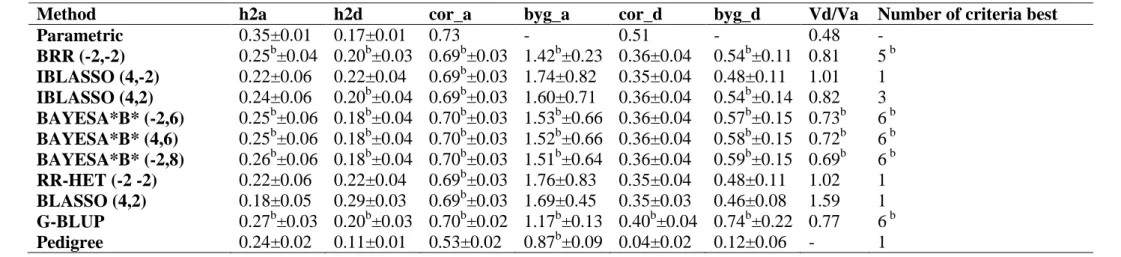
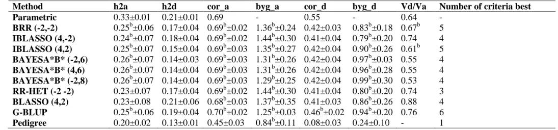
A complete approach for genome-wide selection (GWS) involves reliable statistical genetics models and methods. Reports on this topic are common for additive genetics models but not for additive-dominance models. This paper aimed at: (i) comparing the performance of 10 additive-dominance prediction models (including current ones and proposed modifications), fitted through Bayesian, Lasso and Ridge regression approaches; (ii) decomposing genomic heritability and accuracy in terms of the three quantitative genetics information compounds named linkage disequilibrium (LD), co-segregation (CS) and pedigree relationships or family structure (PR). The simulation study considered two broad sense heritability levels (0.30 and 0.50, associated to narrow sense heritabilities of 0.20 and 0.35, respectively) and two genetic architecture (the first one consisting of small gene effects and the other one with mixed inheritance model with five major genes) for the traits.
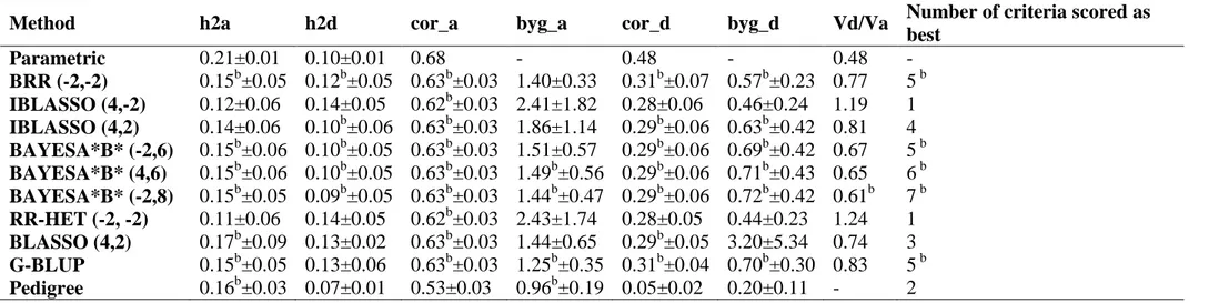
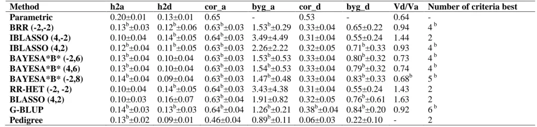
Results
32
genetic architectures). The BayesA*B*-type methods showed better ability for recovering the dominance variance/additive variance ratio. The decomposition of genomic heritability and accuracy revealed the following descending importance order of information: LD, CS and PR not captured by markers, being these last two very close.
Conclusions
Amongst the 10 models/methods evaluated, the G-BLUP, BAYESA*B* (-2,8) and BAYESA*B* (4,6) methods presented the best results and were found to be adequate for accurately predicting genomic breeding and total genotypic values as well as for estimating additive and dominance in additive-dominance genomic models.
Key words: Dominance Genomic Models; Bayesian Methods; Lasso Methods; Selection Accuracy.
1. Background
Genome wide selection (GWS) concerns to phenotype prediction and relies on simultaneous prediction of a great amount of molecular markers effects, thus characterizing as a new paradigm in quantitative genetics (Meuwissen et al., 2001; Gianola et al., 2009) and plant and animal breeding (Goddard and Hayes, 2007; Meuwissen, 2007; Van Raden, 2008; Resende et al., 2008; Grattapaglia and Resende, 2011; Endelman and Jannink, 2012; Resende Jr. et al., 2012a and b).
33
Recent methodologies for GWS and GWAS has been evaluated through simulation studies (Piccoli et al., 2014; Talluri et al., 2014). Simulation and practical results with additive models in GWS with several organisms are common (Van Raden et al. , 2009; Hayes et al., 2009; Grattapaglia and Resende, 2011; Silva et al., 2011; Resende et al., 2012; Resende Jr. et al., 2012a and b; Oliveira et al., 2012; Zapata-Valenzuela et al., 2013; Muñoz et al., 2014). But additive-dominance models are much less common (Zeng et al., 2013; Muñoz et al., 2014; Su et al., 2012; Denis and Bouvet, 2013).
Hill et al. (2008), Bennewitz and Meuwissen (2010) and Wellman and Bennewitz (2012) discussed the relevance of dominance models for the Quantitative Genomics and Genetics. Wellmann and Bennewitz (2012) presented theoretical genetic models for Bayesian genomic selection with dominance and concluded that dominance enhances the analysis and several advantages are aggregated.
Wang and Da (2014) established the correct definitions of genomic relationships and inbreeding, which came to unify the prediction models for additive-dominance genomic selection. Da et al. (2014) and Wang et al. (2014) presented software for additive-dominance models in the framework of the G-BLUP method. Zapata-Valenzuela et al. (2013) also tried to fit additive-dominance models but convergence failed for the main traits.
34
genomic selection in perennials and asexually propagated crops and also in crossed animals.
Bayesian, Lasso and Ridge regression approaches have not been compared for additive-dominance models yet. Zeng et al. (2013), Muñoz et al. (2014), Su et al. (2012) and Denis and Bouvet (2013) and Wang and Da (2014) applied only the G-BLUP method, which is an equivalent model (Goddard et al., 2009), to ridge regression (RR-BLUP). On the other hand, Wellmann and Bennewitz (2012) applied only the Bayesian methods of Meuwissen et al. (2001) with modifications (mixture of two t distributions, one of them with a small variance). Toro and Varona (2010) evaluating the introduction of the dominant effects in the model using the Bayes A. Lasso methods seem to be unused with dominance models for variance components in genomic selection. The study of partition of accuracy and heritability due to the three quantitative genetics information, linkage disequilibrium (LD), co-segregation (CS) and pedigree relationships (PR) has been explored only by Habier et al. (2013).
35 2. Methods
2.1. Simulated datasets
Two random mating populations in linkage equilibrium were crossed generating a population (of size 5,000, coming from 100 families) with linkage disequilibrium (LD), which was subjected to five generations of random mating without mutation, selection or migration. The resultant population is an advanced generation composite, which presents Hardy-Weinberg equilibrium and LD. According to Viana (2004), the LD value () in a composite population is
1 2
1 2
1 2
4 ab
a a b b
p p p p
ab
, where a and b are two SNPs, two QTLs, or one SNP and one QTL, θ is the frequency of recombinant gametes, and p1 and p2 are the allele frequencies in the parental populations (1 and 2). Notice also that the LD value depends on the allele frequencies in the parental populations. Thus, regardless of the distance between the SNPs and/or QTLs, if the allele frequencies are equal in the parental population, Δ = 0. The LD is maximized (|Δ| = 0.25) when θ = 0 and |p1 - p2| = 1. In this case, the LD value is positive with coupling and negative with repulsion (Viana, 2004).
36
small effective population size (Ne = 39.22) and a large LD in the breeding populations. Ne of approximately 40 and the use of 50 individuals per family are typical values in elite breeding populations of plant species (Resende, 2002).
The QTLs were distributed in the regions covered by the SNPs. For each trait, we informed the degree of dominance (d/a being a and d are the genotypic values for one homozygote and heterozygote, respectively) and the direction of dominance (positive and/or negative). The obtained genotypic values for homozygotes were within the limits of Gmax = 100(m + a) and Gmin = 100(m - a) where m is the mean of genotypic values, which are the maximum and minimum values, respectively.
Goddard et al. (2011) presented the realized proportion (rmq2 ) of genetic
variation explained by the markers as mq2
QTL
n r =
n+ n , where nQTLis the number of QTL and n is the number of markers. With n = 2,000 markers and nQTL= 100, we
have 2
0.95 mq
r = . An alternative Hayes et al. (2009) takes
2 2 (39.22) 2 156.88
QTL
n = NeL= = , where L is the total length of the genome (in Morgans), producing 2
0.93 mq
r = . Another approach Sved (1971) provides 2 mq r as
2 1 1
0.86,
1 4 1 4 (39.22) 0.001
mq
r = = =
+ NeS + where S is the distance between markers
(in Morgans). These values reveal that the genome was sufficiently saturated by markers.
37
setting). For the latter, small additive effects were assigned to the remaining 95 loci. The effects were normally distributed with zero mean and genetic variance (size of genetic effects) allowing the desired heritability level. The phenotypic value was obtained by adding to the genotypic value a random deviate from a normal distribution N(0,σe2), where the variance σe2 was defined according to two levels of broad-sense heritability, 0.30 and 0.50, associated with narrow-sense heritabilities of approximately 0.20 and 0.35, respectively. Heritability levels were chosen to represent one trait with low heritability and another with moderate heritability, which addressed the cases where genomic selection is expected to be superior to phenotypic selection (Meuwissen et al., 2001). The magnitudes of the narrow-sense and broad-sense heritabilities are associated with an average degree of dominance level (d/a) of approximately 1 (complete dominance) in a population with intermediate allele frequencies. Simulations assumed independence of additive and dominance effects, with dominance effects having the same distribution as the additive effects (both were normally distributed with zero mean). In the simulation, it was also observed that marker alleles had minor allele frequency (MAF) greater than 5%.
The data were simulated using the RealBreeding software (Viana, 2011).
2.2. Scenarios
38 Table 1. Softwares.
Method Full Name of the Method Class of Methods DF1 DF2 Software
BRR (-2,-2) Bayesian Ridge Regression Bayesian -2 -2 GS3
IBLASSO (4,-2) Improved Bayesian Lasso Bayesian Lasso 4 -2 GS3
IBLASSO (4,2) Improved Bayesian Lasso Bayesian Lasso 4 2 GS3
BAYESA*B* (-2,6) IBLASSO with
t distribution Bayesian Lasso -2 6 GS3
BAYESA*B* (4,6) IBLASSO with
t distribution Bayesian Lasso 4 6 GS3
BAYESA*B* (-2,8) IBLASSO with
t distribution Bayesian Lasso -2 8 GS3
RR-HET (-2, -2) RR-BLUP with
heterogeneous variance Ridge Regression -2 -2 GS3
BLASSO (4,2) Bayesian Lasso Bayesian Lasso 4 2 BLR-R
G-BLUP Genomic BLUP Random Regression - - GVC
Pedigree-BLUP Pedigree-BLUP Random Regression - - Pedigreemm-R
Description of the fitted models and softwares used.
DF1: Degrees of Freedom of the chi-square prior distribution for the residual variance;
DF2: Degrees of Freedom of the chi-square prior distribution for genetic variance or shrinkage parameter.
2.3. Statistical Methods for Additive-Dominance Models
2.3.1. Additive-Dominance Model for the REML/G-BLUP method A mixed linear model for individual additive breeding values (u ) and a dominance deviations (u ) is as follow d y Xb Zu aZude, with variance structure given by a~ 0, a u2 )
a
u N( Gσ ; d~ 0, d u2 )
d
u N( G σ ; e N(~ 0,Iσe2) . An equivalent
39
2
.
a a
2
a ma ma
d d
2 2
d md md
u = Wm ;
Var(Wm )= WIσ W' =WW'σ ν u = Sm ;
Var(Sm )= SIσ S' = SS'σ
W and S are, respectively, the incidence matrices for the vectors of additive (m ) and dominance (a m ) marker genetic effects. The variance components d associated to these effects are 2m
a
σ and m2
d
σ , respectively. G and a G are the d
genomic relationship matrices for additive and dominance effects. The quantity m a in one locus is the allele substitution effect given by m =ai α = a +(q p )di i i i i, where pi and qi are allelic frequencies and a and i d are the genotypic values of one of the i
homozygotes and heterozygote, respectively, at the locus i. By its turn, the quantity
d
m can be directly defined as m = d . di i
The matrices W and S, which will be defined later, are based on the values 0, 1 and 2 for the number of one of the alleles at the i marker locus (putative QTL) in a diploid individual. Several parameterizations are available and the one that matches well with the classical quantitative genetics theory (Falconer and Mackay, 1996) is as follows (Van Raden, 2008;Vitezica, 2013; Wang and Da, 201; Da et al., 2014).
Fitting the individual genomic model is the same as fitting the traditional animal model but with the pedigree genetic relationship matrices A and D replaced by the genomic relationship matrices G and a G for additive and dominance effects, d respectively. The covariance matrix for the additive effects is given by
2 2
a a a ma
Gσ =Var(Wm )=WW'σ , which leads to 2 2 '/ /
a a ma
G = WW (σ σ )
1
'/ 2p 1
n
i i
i=
= WW
[ ( p )], since 2 21
2p 1 n
a i i ma
i=
40
the dominance effects is given by 2 2
d d d md
G σ =Var(Sm )= SS'σ . So
2 2 2
1
´/ / '/ 2p 1
n
d d md i i
i=
G = SS (σ σ )= SS
[ ( p )] , since 2 2 21
2p 1 n
d i i md
i=
σ =
[ ( p )] σ . Thecorrect parameterization in W and S is as follows, according to marker genotypes in a locus i.
If MM, then 2 2 2
If Mm, then 1 2 (1)
If mm, then 0 2 2
p q
W p q p
p p 2 2
If MM, then 0 2
If Mm, then 1 2 (2)
If mm, then 0 2
q S pq p
Additive-dominance G-BLUP method was fitted using the GVC-BLUP software (Wang et al., 2014) via REML through mixed model equations.
2.3.2. Bayesian Ridge Regression (BRR) Method
A Bayesian additive-dominance G-BLUP or Bayesian Ridge Regression (BRR) method was fitted using the GS3 software (Legarra et al., 2013) via MCMC-REML/BLUP assigning flat (i.e. with degrees of freedom equal to -2 which turns out the inverted chi-square into a uniform distribution) prior distributions for variance components (the priori flat is the noninformative priori).
2.3.3. BayesA and BayesB methods