CLM4-BeTR, a generic biogeochemical transport and reaction module for CLM4: model development, evaluation, and application

(1)

GMDD

5, 2705–2744, 2012

CLM4-BeTR for biogeochemical

reaction and transport

J. Tang et al.

Title Page

Abstract Introduction

Conclusions References

Tables Figures

◭ ◮

Back Close

Full Screen / Esc

Printer-friendly Version Interactive Discussion

Discussion

P

a

per

|

Dis

cussion

P

a

per

|

Discussion

P

a

per

|

Discussio

n

P

a

per

|

Geosci. Model Dev. Discuss., 5, 2705–2744, 2012 www.geosci-model-dev-discuss.net/5/2705/2012/ doi:10.5194/gmdd-5-2705-2012

Geoscientific Model Development Discussions

This discussion paper is/has been under review for the journal Geoscientific Model Development (GMD). Please refer to the corresponding final paper in GMD if available.

CLM4-BeTR, a generic biogeochemical

transport and reaction module for CLM4:

model development, evaluation, and

application

J. Tang, W. J. Riley, C. D. Koven, and Z. M. Subin

Department of Climate and Carbon Sciences, Earth Sciences Division, Lawrence Berkeley National Lab (LBL), Berkeley, CA, USA

Received: 7 August 2012 – Accepted: 25 August 2012 – Published: 10 September 2012

Correspondence to: J. Tang (jinyuntang@lbl.gov)

(2)

GMDD

5, 2705–2744, 2012

J. Tang et al.

Title Page

Tables Figures

◭ ◮

Back Close

Full Screen / Esc

Discussion

P

a

per

|

Dis

cussion

P

a

per

|

Discussion

P

a

per

|

Discussio

n

P

a

per

|

Abstract

To improve regional and global biogeochemistry modeling and climate predictability, we have developed a generic reactive transport module for the land model CLM4 (called CLM4-BeTR (Biogeochemical Transport and Reactions)). CLM4-BeTR represents the transport, interactions, and biotic and abiotic transformations of an arbitrary number

5

of tracers (aka chemical species) in an arbitrary number of phases (e.g. dissolved, gaseous, sorbed, aggregate). An operator splitting approach was employed and con-sistent boundary conditions were derived for each modeled sub-process. Tracer fluxes, associated with hydrological processes such as surface run-on and run-off, below-ground drainage, and ice to liquid conversion were also computed consistently with

10

the bulk water fluxes calculated by the soil physics module in CLM4. The transport code was evaluated and found be in good agreement with several analytical test cases. The model was then applied at the Harvard Forest site with a representation of depth-dependent belowground biogeochemistry. The results indicated that, at this site, (1) CLM4-BeTR was able to simulate soil-surface CO2 effluxes and soil CO2

pro-15

files accurately; (2) the transient surface CO2 effluxes calculated based on the tracer

transport mechanism were in general not equal to the belowground CO₂ production rates and that their differences varied according to the seasonal cycle of soil physics and biogeochemistry; (3) losses of CO2 through processes other than surface gas

ef-flux were less than 1 % of the overall soil respiration; and (4) the contributions of root

20

respiration and heterotrophic respiration have distinct temporal signals in surface CO2

effluxes and soil CO2 concentrations. The development of CLM4-BeTR will allow

(3)

GMDD

5, 2705–2744, 2012

J. Tang et al.

Title Page

Tables Figures

◭ ◮

Back Close

Full Screen / Esc

Discussion

P

a

per

|

Dis

cussion

P

a

per

|

Discussion

P

a

per

|

Discussio

n

P

a

per

|

1 Introduction

The trajectory of ongoing climate change (Intergovernmental Panel on Climate Change (IPCC), 2007) depends strongly on greenhouse gas (e.g. H2O, CO2, CH4, and N2O)

exchanges between the terrestrial biosphere and atmosphere. Globally, gross terres-trial ecosystem greenhouse gas fluxes are at least an order of magnitude larger than

5

anthropogenic emissions and have strong climate sensitivity, which can lead to positive feedbacks with the atmosphere (e.g. Cox et al., 2000; Torn and Harte, 2006). Thus, ac-curately modeling terrestrial biogeochemistry is a critical component of earth system models (Friedlingstein et al., 2006).

Much effort has been dedicated to designing terrestrial biogeochemistry models that

10

account for hydrological, energy, and carbon and nitrogen dynamics (e.g. Randerson et al.; 1997; Thornton et al., 2002, 2007; Zhuang et al., 2003; and many others). Many of these existing efforts have used, in each terrestrial gridcell, a single vertically in-tegrated layer for soil biogeochemistry, which we refer to here as a “bucket formu-lation”, as it is analogous to the single-layer hydrology used in early

soil-vegetation-15

atmosphere transfer (SVAT) models. This formulation is insufficient to resolve the depth-dependent soil biogeochemistry, which depends on interactions between the atmosphere, plants, and soils. A good example for the deficiency of the bucket for-mulation is the treatment of wetland ebullition of trace gases, such as methane (CH₄). A sufficient amount of volatile gases produced from different biogeochemical processes

20

needs to accumulate before the gas column becomes unstable such that convection can be triggered to move the gas from the deep soil up to the soil surface quickly. The convection process can vary drastically under different atmospheric and soil physical conditions, with ebullition happening in some cases and not others, despite similar total soil gas pressures (e.g. Tokida et al., 2007). Another example is the characterization of

25

(4)

GMDD

5, 2705–2744, 2012

J. Tang et al.

Title Page

Tables Figures

◭ ◮

Back Close

Full Screen / Esc

Discussion

P

a

per

|

Dis

cussion

P

a

per

|

Discussion

P

a

per

|

Discussio

n

P

a

per

|

Riley et al., 2011; Grant and Roulet, 2002; Maggi et al., 2009). In addition, the existing bucket-type models cannot simulate biogeochemical variables that are directly compa-rable with measurements. For example, the CO2from soil respiration is often assumed

to be measurable at the soil surface instantly after the plant root and soil microorgan-isms produce it, although the characteristic time for transport from the surface to 20 cm

5

in a sandy loam soil at 60 % water-filled pore space, for example, is ∼10–20 h, de-pending on the model used to calculate gas-phase diffusivity (Riley, 2005). As such, the bucket-type models cannot resolve episodic greenhouse gas emissions such as those due to freeze-thaw cycles (e.g. Mastepanov et al., 2008). And because of this, incorrect parameterizations may occur when the soil surface gas efflux measurements

10

are used to calibrate the biogeochemistry submodel.

Depending on the philosophy of the model developers and the model’s intended applications, soil biogeochemistry can be represented with different conceptual struc-tures and model complexities. A few attempts have been made to model the soil-plant-atmosphere exchange of trace gases using a reactive transport modeling (RTM)

ap-15

proach (e.g. Simunek and Suarez, 1993; Fang and Moncrieff, 1999; Grant et al., 1993; Walter and Heimann, 2000; Tang et al., 2010; Wania et al., 2010; Riley et al., 2011). However, the majority of carbon cycling models still have the one-layer bucket struc-ture, such as the Terrestrial Ecosystem Model (e.g. Zhuang et al., 2003), CENUTRY (e.g. Kelly et al., 1997), CASA (e.g. Potter et al., 2003), and CN (e.g. Thornton et al.,

20

2007).

For example, most existing methane models focus either only on CH4, or on both

CH₄ and oxygen (O₂), where the latter is used to determine when a given soil layer, or fraction of the soil layer, is sufficiently aerobic or anaerobic to support the activities of methanotrophs or methanogens. The ability to represent biogeochemical processes

25

(5)

GMDD

5, 2705–2744, 2012

J. Tang et al.

Title Page

Tables Figures

◭ ◮

Back Close

Full Screen / Esc

Discussion

P

a

per

|

Dis

cussion

P

a

per

|

Discussion

P

a

per

|

Discussio

n

P

a

per

|

a system with up to four chemical species (CH₄, CO₂, N₂, and O₂) in gaseous and aqueous phases and considered different conceptual structures to enable a hierarchi-cal modeling of methane dynamics. This allowed them to explore how methane dy-namics depended on the different processes being represented. Still, processes such as adsorption and desorption were not considered there, because no sportive species

5

such as NH+₄ or Dissolved Organic Carbon (DOC) were involved in their study, which are critical for a mechanistic modeling of the nitrogen cycle (e.g. Maggi et al., 2008; Gu et al., 2009).

Field studies also indicate that it is important to consider slower processes such as bio-turbation (e.g. Yoo et al., 2011) and cryoturbation (e.g. Kaiser et al., 2007) in

10

order to correctly model biogeochemistry in some terrestrial ecosystems. However, to our knowledge, no current model exists that integrates both slow and fast processes contributing to vertical differences in biogeochemical cycling.

As understanding of terrestrial ecosystem processes improve, we face the situation of revising biogeochemistry models to incorporate new processes while not losing the

15

legacy of previous model development (see Schmidt et al., 2011 for a perspective dis-cussion on such needs). This situation motivates the development of a generic model template that can relatively easily accommodate new model structures and processes. To meet this and other challenges discussed above, we present here the development of CLM4-BeTR, which includes a flexible modeling structure of terrestrial ecosystem

20

biogeochemistry and a generic multi-phase reaction and transport capability. CLM4-BeTR is integrated in CLM4 (Oleson et al., 2010), the land model of the Earth Sys-tem Model CESM1.0, thereby allowing simulations that integrate processes involving plants, soils, ocean, atmosphere, urban areas, and land and sea ice. We organize the paper as follows: Sect. 2 describes model structure and parameterization, numerical

25

(6)

GMDD

5, 2705–2744, 2012

J. Tang et al.

Title Page

Tables Figures

◭ ◮

Back Close

Full Screen / Esc

Discussion

P

a

per

|

Dis

cussion

P

a

per

|

Discussion

P

a

per

|

Discussio

n

P

a

per

|

2 Model description

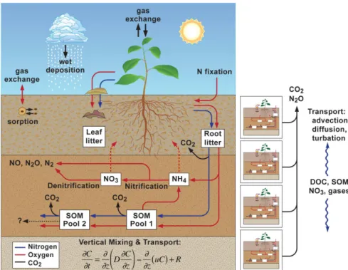
CLM4-BeTR is designed to use a hierarchy of subsurface biogeochemistry models with different levels of complexity and structures and to couple the biogeochemical pro-cesses tightly with the physical propro-cesses, such that model predictions are as relevant as possible to what can be measured in field experiments (Fig. 1). Starting from the

5

atmosphere, we consider tracers (i.e. any chemical species of interest) precipitated to the soil surface and plant canopy through both dry and wet atmospheric deposition. Volatile tracers such as CO2and water vapor are allowed to pass through stomata and

enter leaves. Liquid and solid aqueous tracers are allowed to drip offleaves and onto the soil surface. As in the default CLM4, plant litter falls onto the ground and proceeds

10

through a cascade of decomposition. With the microbially-regulated decomposition of litter-derived organic matter and of plant root exudates, relevant tracers are released into the soil and are allowed to move and interact with flowing water and other chemical tracers through both biogeophysical and biogeochemical pathways. All dissolved trac-ers are allowed to move out of the soil column when the water is drained away, through

15

both over-surface and sub-surface runoff. Volatile tracers are allowed to evaporate back into the soil pore space and atmosphere, and diffuse between the two. Overall, we tried to make the framework sufficiently general that it can tightly couple the various compo-nents of a soil-plant-atmosphere system and track the physical, biophysical, chemical, biochemical, and biological dynamics of an arbitrary number of tracers. With this

struc-20

ture, it will be possible to extend the depth-resolved modeling approach from the soil into the canopy air and connect with the atmospheric chemistry and physics.

Below, we first derive the lumped equations for the reactive transport system. Based on the physical characteristics of the different processes, the operator splitting ap-proach (e.g. Strang, 1968) is applied to solve the governing equations. Consistent

25

(7)

GMDD

5, 2705–2744, 2012

J. Tang et al.

Title Page

Tables Figures

◭ ◮

Back Close

Full Screen / Esc

Discussion

P

a

per

|

Dis

cussion

P

a

per

|

Discussion

P

a

per

|

Discussio

n

P

a

per

|

equations, followed by descriptions of the methods used to diagnose tracer fluxes as-sociated with belowground water flow.

2.1 The governing equation

A general reactive-transport model that considers the transport of multiphase chemical species can be derived from the non-steady mass balance relationship (here for three

5

phases: solid (meaning mineral associated), aqueous, and gaseous):

∂

∂t Cs+θCw+εCg

= ∂

∂z

Ds

∂Cs

∂z

+ ∂

∂z

θDw

∂Cw

∂z

+ ∂

∂z θDg

∂Cg

∂z

!

(1)

−

∂uwCw

∂z −

∂ugCg

∂z +R

whereC_x,x=s, w, g (mol tracer m−3_{) are tracer concentrations in solid, aqueous, and} 10

gaseous phases, respectively;D_x,x=s, w, g (m2s−1_{) are di}

ffusivities for tracers in solid, aqueous, and gaseous phases, respectively;ux,x=w, g (m s−

1

) are the advective ve-locities for aqueous and gaseous tracers, respectively, which are provided by the soil physics model; θ (m3m−3_{) is the water filled soil porosity;} _ε _(m3_m−3_{) is the air filled}

porosity;z (m) is the spatial coordinate (positive upward);t(s) represents time; andR 15

(mol tracer m−3_s−1_{) defines the net tracer production rate at time}_t_{and depth}_z_{. Other}

soil processes such as erosion (Nearing et al., 1994), aggregation and disaggregation (Heuvelink and Pebesma, 1999), sedimentation transport (Merritt et al., 2003), and bioclogging (e.g. Maggi and Porporato, 2007) could also be incorporated into Eq. (1), provided the soil physical processes are modeled consistently. The tracer movement

20

due to horizontal water flow is treated as a separate process and described in Sect. 2.4. In Eq. (1), we considered diffusive and advective transport of aqueous and gaseous tracers. The vertical movement of adsorbed (s) phase is parameterized as a diffusive process (Koven et al., 2009). The reaction termR includes both net chemical produc-tion inside the soil and fluxes due to plant roots, e.g. autotrophic respiraproduc-tion, exudaproduc-tion,

(8)

GMDD

5, 2705–2744, 2012

J. Tang et al.

Title Page

Tables Figures

◭ ◮

Back Close

Full Screen / Esc

Discussion

P

a

per

|

Dis

cussion

P

a

per

|

Discussion

P

a

per

|

Discussio

n

P

a

per

|

and possible transpiration induced fluxes, e.g. NO−

3 uptake through roots (Plhak, 2003)

and soil CO₂transport through root systems into xylem water (Teskey, 2008).

Equation (1) is sufficiently general that it can represent the transport of any well-defined chemical tracer. For example, by ignoring the transport of water vapor in soil, Eq. (1) is reduced to the soil water budget equation currently implemented in CLM4,

5

∂

∂t(Cs+θCw)=−

∂uwCw

∂z −qT (2)

whereCsandCweffectively represent the molar concentrations of ice and liquid water,

respectively andqT (mol water m− 3

s−1_{) represents the sink of water due to}

transpira-tion.

We adopted the fast equilibrium assumption, i.e. equilibrium of tracer concentrations

10

between phases is instantaneously achieved (e.g. Maggi et al., 2008). For instance, NH3 is considered to exist in three phases in equilibrium: gaseous, lumped aqueous,

and adsorbed solid. The lumped aqueous phase includes both NH₄OH and free NH+₄, whose relative concentrations are determined by the equilibrium stoichiometry

NH4OH↔NH+₄+OH− (3)

15

Adopting Eq. (3) enables one to group NH4OH and NH+4 into a single tracer

NHX₄

w,

which is related to NH4OH through

h NHX₄

w

i

=kNH₃,NH+₄[NH4OH] (4)

where the equilibrium constantkNH₃,NH+₄ (unitless) is a function of pH and temperature.

Further, invoking Henry’s law, one has [NH4OH]=B

h (NH3)g

i

, where B (unitless) is the

20

Bunsen solubility coefficient. Therefore, we have the bulk concentration of NHX₄

h

NHX₄i₌θhNHX₄

w

i

+εh(NH3)g

i

+ NH+₄

ads

(9)

GMDD

5, 2705–2744, 2012

J. Tang et al.

Title Page

Tables Figures

◭ ◮

Back Close

Full Screen / Esc

Discussion

P

a

per

|

Dis

cussion

P

a

per

|

Discussion

P

a

per

|

Discussio

n

P

a

per

|

as the single state variable to represent the chemical species related to NH3. In Eq. (5),

NH+₄

ads is the adsorbed phase that is assumed to be in equilibrium with free NH

+

4

dissolved in water, with a sorption parameter dependent on pH, soil texture, and soil organic matter content.

Similarly, the bulk concentration of COX₂ is defined as

5

COX₂=θhCOX₂

w

i

+εh(CO₂)_gi=θ

H₂CO₃ +

HCO−

3

+hCO2−

3

i

+εh(CO₂)_gi(6)

where the relative concentrations of H₂CO₃, HCO−

3, and CO 2₋

3 are determined by their

equilibrium stoichiometry (e.g. Maggi et al., 2008; Gu et al., 2009).

2.2 Numerical implementation

We used the operator splitting approach to solve Eq. (1), which allowed us to use

10

standard numerical solvers to deal with different processes while maintaining numerical efficiency. We grouped the various processes into three different terms, allowing us to rewrite Eq. (1) as

∂Cblk

∂t =Dif+Adv+R (7)

whereCblk(mol tracer m− 3

) is the bulk tracer concentration, including contributions from

15

all possible phases; Dif, Adv, and R represent, respectively, the impacts of diffusion, advection, and reaction (mol tracer m−3_s−1_).

With the Strang splitting approach (Strang, 1968), Eq. (7) can be represented as

Cblk(t+ ∆t)= Dif,∆t/2

Adv,∆t/2 R,∆t/2 Adv,∆t/2 Dif,∆t/2 (8)

where (x,∆t) denotes the integration of process x over a time step ∆t (s), using the

20

(10)

GMDD

5, 2705–2744, 2012

J. Tang et al.

Title Page

Tables Figures

◭ ◮

Back Close

Full Screen / Esc

Discussion

P

a

per

|

Dis

cussion

P

a

per

|

Discussion

P

a

per

|

Discussio

n

P

a

per

|

The soil physics module in CLM4 provides necessary information to drive the integrals in Eq. (8). The vertical advective velocity of liquid water is obtained by solving the Richards’ equation. Aqueous and gaseous tracer diffusivities are com-puted as a function of soil moisture and soil temperature (Appendix A). The solid phase tracer (including adsorbed phase) diffusion is considered as a much slower

5

process (e.g. Koven et al., 2009), such that it can be separated from Eq. (8) and be conducted after the movement of aqueous and gaseous tracers. Specifically, by writing the diffusion processes in Eq. (8) as Dif,∆t/2= Difs,∆t/2

Difgw,∆t/2

, where Difs represents diffusion of solid phase tracer, and Difgw represents diff

u-sion of aqueous and gaseous phase tracer, it can then be shown that C_blk(t+ ∆t)=

10

Dif_s,_∆t/2

C∗

blk(t+ ∆t) Difs,∆t/2

, where C∗

blk(t+ ∆t) represents the tracer update

due to processes other than solid phase diffusion. Thus, because the temporal up-dating of the tracer concentration is done iteratively, the solid phase tracer diffusion becomes a process that can be split from others.

2.2.1 Diffusive transport 15

The Crank-Nicolson (e.g. Press et al., 1986) approach was used to solve the diff u-sion process. In contrast to previous approaches, which only consider the existence of a single water table level (or, more generally, wetting front) and restrict it to the con-necting interface between two consecutive grid layers, in this study we allow multiple water table levels to coexist inside the soil (to accommodate the existence of perched

20

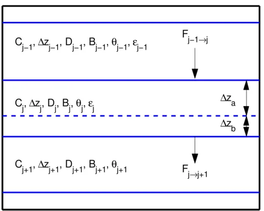
water table), and they can be within the grid layer rather than being restricted to the grid interface. However, only one wetting front is allowed to exist in a single grid layer, though our approach is extendable to consider more general cases. Specifically, the incoming flux from layerj−1 to layerj (j increases with depth) is computed as (Fig. 2)

25

Fj−1→j =−r

−1

j−1 aCj−Cj−1

(11)

GMDD

5, 2705–2744, 2012

J. Tang et al.

Title Page

Tables Figures

◭ ◮

Back Close

Full Screen / Esc

Discussion

P

a

per

|

Dis

cussion

P

a

per

|

Discussion

P

a

per

|

Discussio

n

P

a

per

|

and the outgoing flux from layerj to layerj+1 is computed as

F_j_→_j₊1=−r_j−1 Cj+1−bCj

(10)

where

r_j₋1=

∆z_j₋1

2D_j₋1

+ ∆za 2D_j,a

+ ∆zb 2D_j,b

B_j₋1θj−1+εj−1

B_jθ_j

!

(11a)

r_j =∆zj+1

2D_j₊1

+ ∆zb 2D_j,b

+ ∆za 2D_j,a

B_j₊₁θ_j₊₁

B_jθ_j+ε_j

!

(11b)

5

a=∆za

∆z_j +

∆zb

∆z_j

B_j₋₁θj−1+εj−1

B_jθ_j

!

(11c)

b=∆za

∆zj

B_j₊₁θj+1

B_jθj+εj

!

+∆zb ∆zj

(11d)

Equations (9)–(11) are used to solve the diffusion of aqueous and gaseous tracer, where we usedCj =θjCw,j+εjCg,j and assumed that transport of the adsorbed phase

10

of the tracer (if it does exist) can be considered separately as justified in the formulation of Eq. (8). When the water table level overlaps the grid interface, Eqs. (9)–(11) become identical to the relationships used in Riley et al. (2011).

2.2.2 Advective transport

In order to be consistent with the way that CLM4 updates soil water content, the

ad-15

vection operator is next solved for soil aqueous phase tracers:

θ∂Cw

∂t =−

∂uwCw

∂z −

qT+

∂θ ∂t

(12)

GMDD

5, 2705–2744, 2012

J. Tang et al.

Title Page

Tables Figures

◭ ◮

Back Close

Full Screen / Esc

Discussion

P

a

per

|

Dis

cussion

P

a

per

|

Discussion

P

a

per

|

Discussio

n

P

a

per

|

Currently, gas advection is accounted for by a pressure adjustment approach (e.g. Tang et al., 2010), such that the gas column is always hydrostatically stable. In future work we will incorporate an explicit Darcy solver for gaseous advection.

Since the soil moisture and water fluxes are updated before the advection of the aqueous tracers, Eq. (12) is solved as

5

θn+1

∆t

Cn+1

w −Cnw

=Un−

qT+

∂θ ∂t

n+1

Cn+1

w (13)

whereUn is the forward-in-time upstream discretization (Tremback et al., 1987) of the advection term in Eq. (12). In the model, whether a particular aqueous tracer is allowed to move with the transpiration flux q_T is set prior to runtime. As such, CLM4-BeTR provides a method to assess the importance of transpiration-induced tracer fluxes.

10

For instance, the movement of soil CO2 into roots and xylem water (Teskey, 2008) or

nutrient uptake in the transpired water flow to meet the plant’s nutrient demand (e.g. Plhak, 2003) can be explored with this model structure by further considering relevant storage pools in plant.

2.2.3 Trace movement in snow 15

The tracer movement associated with snow accumulation and melt are computed in a similar way as for aerosols in CLM4 (Oleson et al., 2010). CLM4 assumes the aerosols are uniformly sorbed to the snow particles and redistributes them according to the change of snow mass, while assuming no diffusive movement of those aerosols. CLM4-BeTR also considers tracer movement through both advection and diffusion,

20

with the snow-sorbed tracer being adjusted using the fast equilibrium approximation.

2.3 Boundary conditions and surface flux calculation

(13)

GMDD

5, 2705–2744, 2012

J. Tang et al.

Title Page

Tables Figures

◭ ◮

Back Close

Full Screen / Esc

Discussion

P

a

per

|

Dis

cussion

P

a

per

|

Discussion

P

a

per

|

Discussio

n

P

a

per

|

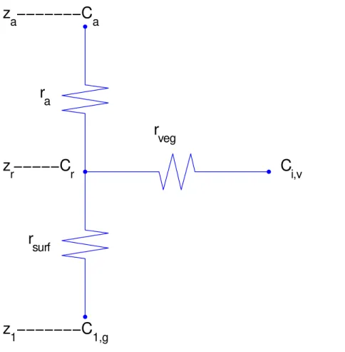
diffusion (including dry deposition), a two-layer model similar to that currently applied for water vapor in CLM4 (Oleson et al., 2010) was adopted, as described below.

We assume the gaseous tracer concentration at the level of the apparent sink (Fig. 3) is computed as

C_r=r_T C1,g

rsurf +

Ci,v

rveg+

Ca

ra

!

(14)

5

where Ci,v (mol tracer m−3; subscript i means inside leaf) is the weighted leaf

inter-nal gas concentration (including contributions from sunlit and shaded leaves, see Ap-pendix B) of a given tracer;Ca (mol tracer m−

3

) is the atmospheric gas concentration; andC1,g(mol tracer m−

3

) is the top soil control volume gas concentration. The surface (rsurf), vegetation (rveg), and weighted bulk (rT) resistances (s m−

1

) are defined as

10

rsurf= ra,s+rb,s+rs,s

+ ∆z1

2D1(B1θ1+ε1)

(15)

rveg=rb,v+rs,v (16)

rT =

1

rsurf+

1

rveg+

1

ra

−1

(17)

wherera,s (s m− 1

) is the aerodynamic resistance inside the canopy air;rb,s (s m− 1

) is

15

the soil surface laminar boundary layer resistance; rs,s (s m− 1

) is the resistance due to surface litter (Sakaguchi and Zeng, 2009);ra (s m−

1

) is the aerodynamic resistance above the canopy;rb,v (s m−

1

) is the leaf boundary layer resistance;rs,v (s m− 1

) is the weighted stomatal resistance (Eq. B5 in Appendix B) that includes contributions from sunlit and shaded leaves; and∆z1(m), θ1 (m−

3

water m−3 _soil), _ε

1(m 3

air m−3 _soil), 20

and D1 (m 2

s−1_{) are, respectively, the thickness, water filled porosity, air filled}

(14)

GMDD

5, 2705–2744, 2012

J. Tang et al.

Title Page

Tables Figures

◭ ◮

Back Close

Full Screen / Esc

Discussion

P

a

per

|

Dis

cussion

P

a

per

|

Discussion

P

a

per

|

Discussio

n

P

a

per

|

Eq. (15) is provided in Tang and Riley (2012, A mechanistic top boundary condition for modeling air-soil di_ffusive exchange of a generic volatile tracer: theoretical analysis and application to soil evaporation, under review at Water Resources Research).

The diffusive flux at the soil surface,Fsurf(mol tracer m− 2

s−1_{, positive upward), is:}

Fsurf=−

C_r−C1,g

rsurf

=− rT

rsurf

C

i,v

rveg

+Ca

ra

+C1,g

rsurf

1− rT

rsurf

(18)

5

For a non-vegetated bare soil,rveg is set to infinity andra,s is set to zero, which leads

to the diffusive flux up from the surface:

Fsurf=−

Ca−C1,g

ra+rsurf

(19)

The di_ffusive e_fflux from the vegetationFveg(mol tracer m− 2

s−1_{) is:}

Fveg=−

C_r−Ci,v

rveg

=−

r_T

rveg

C1,g

rsurf

+Ca

ra

!

+Ci,v

rveg

1₋ rT

rveg

(20)

10

The total diffusive flux of the tracer,Ftot(mol tracer m− 2

s−1_{), exchanging with the}

atmo-sphere is:

Ftot=

r_T

ra

C1,g

rsurf +

Ci,v

rveg

!

−

Ca

ra

1−

r_T

ra

(21)

The radiation boundary condition (e.g. Raymond and Kuo, 1984) is applied at the lower boundary. However, since CLM4 has no representation of tracer concentrations

15

(15)

GMDD

5, 2705–2744, 2012

J. Tang et al.

Title Page

Tables Figures

◭ ◮

Back Close

Full Screen / Esc

Discussion

P

a

per

|

Dis

cussion

P

a

per

|

Discussion

P

a

per

|

Discussio

n

P

a

per

|

2.4 Tracer fluxes diagnostics

CLM4-BeTR diagnoses tracer fluxes through different physical pathways explicitly. Tracers from dry and wet deposition to the soil surface are directly added to the first soil (or snow) layer. During snow melting, the aqueous tracers are moved inside the snow layers consistently with liquid water flow. The total aqueous fluxes reaching the

5

soil surface are partitioned into tracer infiltration and run-offloss in accordance with the partitioning of infiltration and surface run-o_ffof liquid water.

To compute horizontal tracer fluxes inside the soil associated with surface runoff, we assumed that aqueous tracers in the first two soil layers (totaling 4.5 cm thick) are in equilibrium with those in the runoff water. The tracer concentrations in these top two

10

soil layers are then updated accordingly. This approach is clearly an approximation and deserves more attention in subsequent model versions.

In order to compute the tracer loss through sub-surface drainage, the fraction of water removed from each hydrologically active layer is tracked explicitly. This fraction of water loss for a given soil layer is then assumed to be equal to the fraction of aqueous

15

tracer being lost, which is then used to compute tracer loss from that specific soil layer. In the current version of CLM4-BeTR, tracer fluxes through dew formation and drip from plant-interception are generically included following the way that CLM4 deals with the water fluxes through those processes, but are considered to be zero in the analyses that follow. For volatile tracers, the surface exchange through diffusion is computed

us-20

ing the gradient-based approach described in Sect. 2.3. Transport through parenchyma or arenchyma is formulated as in Riley et al. (2011). Ebullition is represented using the approach described in Tang et al. (2010), which consideres the pressure contributed from different volatile tracers while imposing no gas volume theresholds as done in Riley et al. (2011).

25

(16)

GMDD

5, 2705–2744, 2012

J. Tang et al.

Title Page

Tables Figures

◭ ◮

Back Close

Full Screen / Esc

Discussion

P

a

per

|

Dis

cussion

P

a

per

|

Discussion

P

a

per

|

Discussio

n

P

a

per

|

provided by the soil physics module is used to determine the effective porosity of the aqueous and gaseous phases. Whether a given dissolved tracer can be locked into ice is a property that needs to be set prior to runtime. If so, the change in ice fraction over a time step is used to update the fraction of the dissolved tracer locked into, or lost from, the ice. When the surface soil layer is completely frozen, tracer di_ffusion to the

at-5

mosphere is suppressed. This model feature (not applied in the analyses here) allows us to explore the effect of freeze-thaw cycles on substrate and nutrient availability for plant roots and soil microorganisms, which we will explore in future studies. However, the current version of the model resolves the episodic gas emissions due to changes in effective soil porosity following freeze-thaw events (e.g. Mastepanov et al., 2007).

10

3 Model evaluation and example applications

Below we first describe the strategies used to evaluate CLM4-BeTR, including a com-parison of numerical and analytical solutions and a comcom-parison of model outputs with site-level measurements at Harvard Forest (http://harvardforest.fas.harvard.edu/). Then we present a simple application to show how the tracer tracking capability can

15

provide new insights into interpretation of tracer concentration and flux measurements and their representation in biogeochemical models such as CLM4.

3.1 Evaluation against analytical solutions

A comparison between the numerical and analytical solutions was conducted to evalu-ate the accuracy of the 1-D transport simulator integrevalu-ated in CLM4-BeTR. We used two

20

di_fferent analytical solutions to evaluate the code. The two analytical solutions satisfy the 1-D reactive transport equation:

∂C

∂t =

∂ ∂z

D∂C

∂z

(17)

GMDD

5, 2705–2744, 2012

J. Tang et al.

Title Page Abstract Introduction Conclusions References Tables Figures ◭ ◮ ◭ ◮ Back Close

Full Screen / Esc

Printer-friendly Version Interactive Discussion Discussion P a per | Dis cussion P a per | Discussion P a per | Discussio n P a per |

with their respective initial conditions and boundary conditions. HereDis diffusivity, and

uis advection velocity (positive downward). In all comparisons between the numerical and analytical solutions, the diffusivity D was set to 10−6_m2_s−1 _{and the advection}

velocityuwas set to 10−7_{m s}−1_{(which is two orders of magnitude greater than typical}

vertical liquid water flows computed by CLM4).

5

For the first analytical solution, a pulse tracer input is imposed at the top of a 1-D column of lengthL, resulting in the tracer concentrationC(mol m−3_):

C=1

2erfc

_z

−ut 2√Dt

+1 2exp uz D erfc _z +ut

2√Dt

+h1+ u

2D(2L−z+ut)

i ·exp _uL D erfc

2L−z+ut 2√Dt

− s

u2_t

πDexp

"

uL

D −

(2L−z+ut)2 4Dt

#

(23)

10

where erfc (x) is the complementary error function of x. For the comparisons, we set

L=42.10 m, corresponding to the maximum depth of the temperature solution cur-rently calculated in CLM4 (computed using Eqs. 6.5–6.7 in Oleson et al., 2010).

For the second analytical solution, the tracer concentration top boundary condition is

C(z=0)=C0+

2

P

i=1

A_iexp −2uD−

√

2 4D

r

u2₊q_u4₊₁₆_D2_ω2

i

!

sin (ω_it) , which leads to

15

the wave type analytical solution:

C=C0+

2

X

i=1

A_iexp − u

2D−

√ 2 4D

r

u2₊

q

u4₊₁₆_D2_ω2

i ! (24) · sin     

ωit−

√ 2ω_iz

r

u2₊q_u4₊₁₆_D2_ω2

(18)

GMDD

5, 2705–2744, 2012

J. Tang et al.

Title Page

Tables Figures

◭ ◮

Back Close

Full Screen / Esc

Discussion

P

a

per

|

Dis

cussion

P

a

per

|

Discussion

P

a

per

|

Discussio

n

P

a

per

|

where A_i,i=1, 2, (mol tracer m−3_{) are the amplitudes and} _ω

i,i =1, 2, (s−

1

) are the frequencies. For the numerical comparison, we set C0=12/23 mol tracer m−

3

, A1=

9/23 mol tracer m−3_, _A

2=2/23 mol tracer m− 3

, ω1=2π/(365×86 400) s− 1

and ω2=

2π/86 400 s−1_{. The values of parameters}_C

0,A1, andA2are chosen to ensure that the

maximum tracer concentration is 1 mol m−3_. 5

3.2 Single point evaluation at the harvard forest site

We conducted a single point simulation at the Harvard Forest site with depth dependent C and N dynamics, which includes a vertical discretization of the soil biogeochemistry, a decomposition cascade, and nitrification and denitrification parameterization based on the CENTURY model (Parton et al., 1988; Del Grosso et al., 2000) for the site level

10

evaluation. The tracer transport capability of CLM4-BeTR was used to evaluate the soil biogeochemistry, which provides the relevant tracer fluxes. A total of six tracers were modeled: N2, O2, Ar, CO

X

2, N2O, and NO. We spun up the model for 1000 yr using

a repeating 57-yr (1948–2004) cycle of meteorological data extracted from the global dataset (Qian et al., 2006). Another 40-yr simulation was then conducted, from which

15

the average of the last 10 yr of model output were compared with the measurements. The measurement data include CO₂ effluxes (as derived ecosystem respiration) from the AmeriFlux dataset (level 4 ecosystem respiration flux data, from year 1992 to 2006; http://public.ornl.gov/ameriflux/dataproducts.shtml) and CO2 profiles collected at the

site from June 1995 to December 2004 (Davidson et al., 2006). Given the uncertainties

20

in meteorological forcing data, model parameterization, and site-model mismatch, we did not try to match the model predictions to the measurements, which would otherwise involve an intensive practice of data assimilation and uncertainty quantification of CLM4 that is beyond the scope of this study. Rather, we grouped the observed daily CO₂eddy flux observations into a single-year time series, and compared it with the simulated

25

(19)

GMDD

5, 2705–2744, 2012

J. Tang et al.

Title Page

Tables Figures

◭ ◮

Back Close

Full Screen / Esc

Discussion

P

a

per

|

Dis

cussion

P

a

per

|

Discussion

P

a

per

|

Discussio

n

P

a

per

|

were grouped into monthly time steps to form a single-year time series to enable the comparison.

3.3 Partitioning of surface CO2fluxes with CLM4-BeTR

To illustrate potential applications of CLM4-BeTR, we designed a tagged CO2 tracer

simulation to visualize the relative contributions of different sources to the measured

5

soil surface CO2fluxes and soil CO2 concentrations. Specifically, using the initial

con-ditions provided from the simulations described in Sect. 3.2, we represented the CO2

originating from three sources: root respiration, soil heterotrophic respiration, and from the atmosphere with three tracers and tracked their temporal and spatial evolutions with CLM4-BeTR. This approach allowed us to partition the predicted soil surface CO2

10

fluxes into contributions from these three sources. We then analyzed whether these three sources have distinct signals from the soil surface CO₂ e_ffluxes and soil CO₂ concentrations measured in the field.

4 Results and discussions

4.1 Evaluation against analytical solutions 15

Comparisons between numerical and analytical solutions indicate the 1-D transport code accurately (root mean square error are less than 0.01 for all cases) represented tracer transport for both the pulse and wave boundary condition simulations using the CLM4 standard vertical discretization and time step (Fig. 4a, c). Refining the vertical resolution (i.e. halving the grid size in the transformed exponential coordinate

sys-20

(20)

GMDD

5, 2705–2744, 2012

J. Tang et al.

Title Page

Tables Figures

◭ ◮

Back Close

Full Screen / Esc

Discussion

P

a

per

|

Dis

cussion

P

a

per

|

Discussion

P

a

per

|

Discussio

n

P

a

per

|

CLM4 vertical grid structure and time-step (30 min) is sufficient to produce reasonable model simulations.

4.2 Single point evaluation at the Harvard Forest site

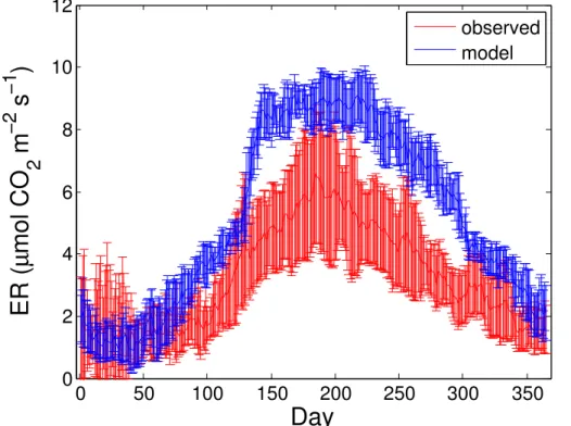
Simulated mean seasonal cycle of ecosystem respiration was generally in good agreement with the data derived from tower eddy flux measurements (Fig. 5).

Start-5

ing from April (day 91), the model simulated higher ecosystem respiration than ob-served, though predicted GPP is close to the measurements (with a linear fitting

x=0.88y−0.8780(µmol CO2m− 2

s−1_{), where}_x_{represents simulated GPP, and}_y

rep-resents the observed data; data not shown). The overestimation in ecosystem respira-tion could be from any of the predicted respiratory components, including above ground

10

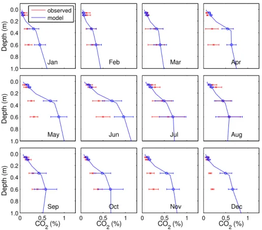
autotrophic respiration, root autotrophic respiration, and soil heterotrophic respiration. We next integrated the predicted belowground CO2 production rate with the

trans-port module in CLM4-BeTR to calculate soil-gas CO2concentrations (Fig. 6). The

pre-dicted soil CO₂concentrations were generally higher than observed from April through June, in relatively good agreement with observations from July through September,

15

and higher than observed from October through December. It is not clear whether the overestimation in soil CO₂ concentrations resulted from an overestimation of the CO₂ production rate in soil heterotrophic respiration or in root autotrophic respiration, or insufficient transport due to incorrect physical forcing, or even some combination that varied with time. However, analyses indicated that the simulated soil temperature

20

was in good agreement with measurement at all four-observation depths (6, 10, 33, and 60 cm), where the soil air samples were taken (Fig. S1). The model simulated soil moisture was higher than observed throughout most of the year (Fig. S2). Hence, ac-cording to the way that the soil moisture a_ffects the tracer transport and organic matter decomposition (Andren and Paustian, 1987) in the model, a reasonable hypothesis is

25

(21)

GMDD

5, 2705–2744, 2012

J. Tang et al.

Title Page

Tables Figures

◭ ◮

Back Close

Full Screen / Esc

Discussion

P

a

per

|

Dis

cussion

P

a

per

|

Discussion

P

a

per

|

Discussio

n

P

a

per

|

a mass budget analysis of the belowground CO₂dynamics indicated that, at this site, the CO2 loss through surface and subsurface runoffis less than 1 % of the total CO2

produced from belowground respiration.

4.3 Partitioning surface CO2fluxes

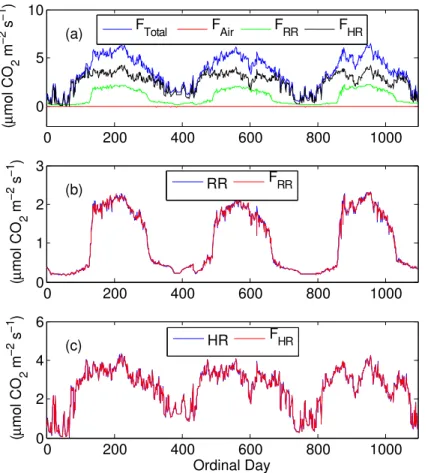
We found the three predicted CO₂ sources (soil heterotrophic respiration, root

respi-5

ration, and atmospheric CO2) differ distinctly in contributing to the overall soil surface

CO2efflux (Fig. 7a). The atmospheric CO2source (denoted by Air) contributed a

neg-ligible amount (being two orders of magnitude smaller than the other two sources), indicating, as expected, that the surface CO2efflux is dominated by belowground

bio-geochemical production. In this simulation, the CO2 produced from soil heterotrophic

10

respiration dominated the total surface efflux, particularly in the non-growing season, when autotrophic root respiration diminished due to reduced vegetation productivity. In addition, due to a tight coupling with soil physics, soil heterotrophic CO2production

was more temporally variable than root autotrophic respiration. However, we are not sure if such behavior is close to what actually occur in the field.

15

At the daily time step, small yet significant discrepancies existed between simu-lated surface CO₂ effluxes and heterotrophic plus autotrophic root CO₂ production rates (Fig. 7b, c). However, more significant discrepancies were identified when the surface CO2 effluxes and total belowground productions rates were compared at the

hourly time scale (Fig. 8a, b). In the growing season (from 1 May to 31 October),

20

we found hourly soil surface CO₂ e_ffluxes were often di_fferent from the belowground CO2 production rate (8b). When the histogram of the relative differences (defined as

(FSR−SR)/FSR×100 %, whereFSR (µmol CO2m− 2

s−1_{) is the surface CO}

2 efflux and

SR (µmol CO₂m−2_s−1_{) is the belowground CO}

2 production) were analyzed for the

growing season, a slightly asymmetric distribution was identified (Fig. 8c), with the soil

25

surface CO2efflux slightly higher (statistically significant at the screen levelp <0.01)

(22)

GMDD

5, 2705–2744, 2012

J. Tang et al.

Title Page

Tables Figures

◭ ◮

Back Close

Full Screen / Esc

Discussion

P

a

per

|

Dis

cussion

P

a

per

|

Discussion

P

a

per

|

Discussio

n

P

a

per

|

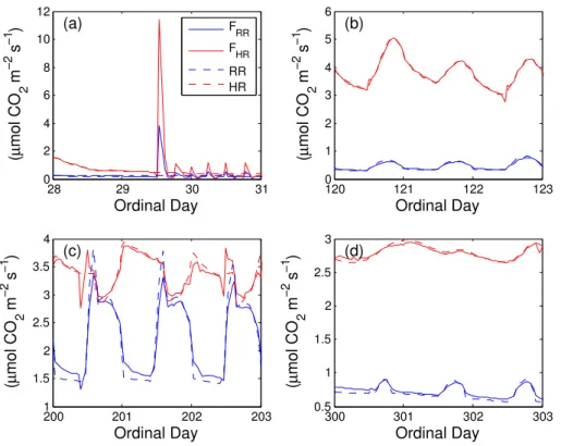
was due to the higher emission than production rate signal in the nighttime (Fig. S3). The relative difference at the hourly scale could be as much as 20 % during the growing season, and up to 80 % during the winter, when freeze-thaw driven episodic emissions occurred (e.g. the peak emission on day 30 in Fig. 8a). When averaged over daily time steps, however, the differences between the surface CO2 effluxes and belowground

5

production were much smaller and showed a more symmetric distribution around the mean zero (Fig. 8c), supporting the finding that the temporal averaging to time scales larger than 24 h could suppress the strong small time step signals in the measured CO2 surface efflux (Fig. 7). The large differences at the hourly time scale indicate

po-tential problems associated with the common approach used to infer GPP from eddy

10

covariance NEE measurements (Desai et al., 2008).

Grouping the relative differences into a monthly time step showed there were sea-sonally systematic biases. In particular, the surface CO2effluxes tended to be smaller

than belowground production during the thaw period, and vice versa during the freez-ing period (Fig. 8d). To better understand these seasonally dependent biases, we

an-15

alyzed hourly time step model predictions for four different three-day periods: the end of January, early May, late July, and late October (Fig. 9). In the thaw season, CO₂ loss through surface and belowground drainage, as well as increased soil gas storage capacity, made the surface CO2 efflux smaller than the total belowground production

rates. However, when temperatures were below freezing (days 28–31 and 300–303),

20

the loss through drainage diminished and the soil gas storage capacity decreased, such that very strong episodic CO2 emissions can occur during the short-term thaw

event between two consecutive freezing events or at the start of the thaw season. Such episodic emissions can be three to four times higher than the CO2 effluxes

dur-ing the peak-growdur-ing season (Fig. 8a and Fig. 9a), and 20 or more times higher than

25

(23)

GMDD

5, 2705–2744, 2012

J. Tang et al.

Title Page

Tables Figures

◭ ◮

Back Close

Full Screen / Esc

Discussion

P

a

per

|

Dis

cussion

P

a

per

|

Discussion

P

a

per

|

Discussio

n

P

a

per

|

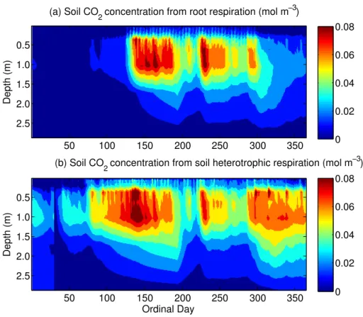
In accordance with the distinct temporal patterns of CO₂ production rates from soil heterotrophic respiration and autotrophic root respiration (Fig. 7), the resulting CO2

concentrations from these two sources also showed distinct temporal patterns (Fig. 10). The CO₂ produced from soil heterotrophic respiration persisted at higher levels over a longer fraction of the year than CO2from root respiration. However, due to the

phys-5

ical transport of the CO2 in the soil profile, we found that the location of high CO2

concentrations usually differed from the CO₂ production hot spots. In addition, when an incorrect top boundary condition or a different root profile was used, the simulated surface CO2 effluxes would not change significantly although the soil CO2

concentra-tions would drastically change (results not shown). These finding indicate that field soil

10

CO₂ concentration measurements can provide additional constraints on belowground biogeochemistry besides that provided from surface CO2efflux measurements.

5 Summary

In this study, we presented methods, testing, and an application of CLM4-BeTR, a gen-eral multi-phase reactive transport model integrated in CLM4. The model is designed to

15

tightly couple depth-dependent biogeochemistry and physics, to use a hierarchy of bio-geochemistry models with different structural complexities, and to readily couple with atmospheric chemistry and physics modules. The comparison with analytical solutions showed the transport calculations were accurate with the default CLM4 time-step and vertical grid structure. An evaluation of modeled surface CO2effluxes and soil CO2

pro-20

files indicates that the model was able to reasonably capture the seasonal dynamics of soil surface CO2 effluxes and soil CO2 concentrations, subject to the

uncertain-ties associated with the measurements and model forcings. The component-wise CO₂ tracer transport experiment indicated that there are timescale-dependent biases be-tween the surface CO2 effluxes and the corresponding belowground CO2 production

25

(24)

GMDD

5, 2705–2744, 2012

J. Tang et al.

Title Page

Tables Figures

◭ ◮

Back Close

Full Screen / Esc

Discussion

P

a

per

|

Dis

cussion

P

a

per

|

Discussion

P

a

per

|

Discussio

n

P

a

per

|

terrestrial biogeochemistry models (more detailed analyses will be conducted in follow-up studies). In future studies, we will present further developments associated with CLM4-BeTR, such as explicit carbon and nitrogen transport, isotope transport and mi-crobial dynamics, that enable a comprehensive and mechanistically-based evaluation of atmosphere-biosphere interactions, involving both physical and chemical feedbacks.

5

Appendix A

Computing the diffusivities

Following the approach by Moldrup et al. (2003), the effective diffusivity for aqueous tracer is computed as

Dw=D∗wθ

θ ϕ

κ/3−1

(A1)

10

The effective diffusivity for gaseous tracer is computed as

Dg=D∗gε

_ε

ϕ

3/κ

(A2)

Here,ϕ(m3m−3_{) is the e}_ff_{ective soil porosity, being equal to the soil porosity minus the}

space occupied by ice.κ (unitless) is the shape parameter for the Clapp-Hornberger parameterization (Clapp and Hornberg, 1978). D∗

w is the aqueous tracer diffusivity in

15

liquid water, andD∗

(25)

GMDD

5, 2705–2744, 2012

J. Tang et al.

Title Page

Tables Figures

◭ ◮

Back Close

Full Screen / Esc

Discussion

P

a

per

|

Dis

cussion

P

a

per

|

Discussion

P

a

per

|

Discussio

n

P

a

per

|

Appendix B

Computing the weighted leaf internal gas concentration

The flux (positive upward) over the sunlit leaf is

Fsun=−r−

1

sun Ci,sun−Cr

(B1)

and the flux over the shaded leaf is

5

Fsha=−r_sha−1 Ci,sha−Cr

(B2)

where the sunlit (rsun) and shaded (rsha) resistance (s m− 1

) are functions of leaf (stem) area index and leaf boundary layer resistance (see Sect. 5.3 in Oleson et al., 2010).

Then the total flux over the canopy is

Fveg=Fsun+Fsha=−

r−1

sun+r− 1 sha

−1 rsun−1Ci,sun+r− 1 shaCi,sha

r−1

sun+r− 1 sha

−Cr

!

(B3)

10

which gives the weighted leaf internal tracer concentration as

Ci,v=

r−1

sunCi,sun+r− 1 shaCi,sha

r−1

sun+r− 1 sha

(B4)

From Eq. (B3), the weighted stomatal resistancers,v(s m− 1

) is found as

rs,v=

1

rsun+

1

rsha

−1

(B5)

Supplementary material related to this article is available online at: 15

(26)

GMDD

5, 2705–2744, 2012

J. Tang et al.

Title Page

Tables Figures

◭ ◮

Back Close

Full Screen / Esc

Discussion

P

a

per

|

Dis

cussion

P

a

per

|

Discussion

P

a

per

|

Discussio

n

P

a

per

|

Acknowledgements. This research was supported by the Director, Office of Science, Office

of Biological and Environmental Research of the US Department of Energy under Contract No. DE-AC02-05CH11231 as part of their Regional and Global Climate Modeling Program. The authors appreciate Ms. Kathleen Savage and Eric Davidson at the Woods Hole Research Center for providing the soil CO₂ profile data and soil moisture and temperature data at the

5

Harvard Forest site.

References

Andren, O. and Paustian, K.: Barley straw decomposition in the field – a comparison of models, Ecology, 68, 1190–1200, 1987.

Clapp, R. B. and Hornberger, G. M.: Empirical equations for some soil hydraulic properties,

10

Water Resour. Res., 14, 601–604, 1978.

Cox, P. M., Betts, R. A., Jones, C. D., Spall, S. A., and Totterdell, I. J.: Acceleration of global warming due to carbon-cycle feedbacks in a coupled climate model, Nature, 408, 184–187, doi:10.1038/35041539, 2000.

Davidson, E. A., Savage, K. E., Trumbore, S. E., and Borken, W.: Vertical partitioning

15

of CO₂ production within a temperate forest soil, Glob. Change Biol., 12, 944–956, doi:10.1111/J.1365-2486.2005.01142.X, 2006.

Del Grosso, S. J., Parton, W. J., Mosier, A. R., Ojima, D. S., Kulmala, A. E., and Phongpan, S.: General model for N₂O and N-2 gas emissions from soils due to dentrification, Global Bio-geochem. Cy., 14, 1045–1060, 2000.

20

Desai, A. R., Richardson, A. D., Mo_ffat, A. M., Kattge, J., Hollinger, D. Y., Barr, A., Falge, E., Noormets, A., Papale, D., Reichstein, M., and Stauch, V. J.: Cross-site evaluation of eddy covariance GPP and RE decomposition techniques, Agr. Forest Meteorol., 148, 821–838, doi:10.1016/J.Agrformet.2007.11.012, 2008

Fang, C. and Moncrieff, J. B.: A model for soil CO₂production and transport, 1: model

develop-25

ment, Agr. Forest Meteorol., 95, 225–236, 1999.

Friedlingstein, P., Cox, P., Betts, R., Bopp, L., Von Bloh, W., Brovkin, V., Cadule, P., Doney, S., Eby, M., Fung, I., Bala, G., John, J., Jones, C., Joos, F., Kato, T., Kawamiya, M., Knorr, W., Lindsay, K., Matthews, H. D., Raddatz, T., Rayner, P., Reick, C., Roeckner, E., Schnitz-ler, K. G., Schnur, R., Strassmann, K., Weaver, A. J., Yoshikawa, C., and Zeng, N.:

(27)

GMDD

5, 2705–2744, 2012

J. Tang et al.

Title Page

Tables Figures

◭ ◮

Back Close

Full Screen / Esc

Discussion

P

a

per

|

Dis

cussion

P

a

per

|

Discussion

P

a

per

|

Discussio

n

P

a

per

|

carbon cycle feedback analysis: results from the C(4)MIP model intercomparison, J. Clim., 19, 3337–3353, 2006.

Grant, R. F.: Simulation-model of soil compaction and root-growth, 1. Model structure, Plant Soil, 150, 1–14, 1993.

Grant, R. F. and Roulet, N. T.: Methane efflux from boreal wetlands: theory and testing of the

5

ecosystem model Ecosys with chamber and tower flux measurements, Global Biogeochem. Cy., 16, 1054, doi:10.1029/2001gb001702, 2002.

Gu, C. H., Maggi, F., Riley, W. J., Hornberger, G. M., Xu, T., Oldenburg, C. M., Spycher, N., Miller, N. L., Venterea, R. T., and Steefel, C.: Aqueous and gaseous nitrogen losses induced by fertilizer application, J. Geophys. Res.-Biogeo., 114, G01006, doi:10.1029/2008jg000788,

10

2009.

Heuvelink, G. B. M. and Pebesma, E. J.: Spatial aggregation and soil process modelling, Geo-derma, 89, 47–65, 1999.

Intergovernmental Panel on Climate Change (IPCC): Climate Change 2007: The Physical Sci-ence Basis. Contribution of Working Group I to the Fourth Assessment Report of the

In-15

tergovernmental Panel on Climate Change, edited by: Solomon, S., Qin, D., Manning, M., Chen, Z., Marquis, M., Averyt, K. B., Tignor, M., and Miller, H. L., Cambridge University Press, Cambridge, UK and New York, NY, USA, 2007.

Kaiser, C., Meyer, H., Biasi, C., Rusalimova, O., Barsukov, P., and Richter, A.: Conservation of soil organic matter through cryoturbation in arctic soils in Siberia, J. Geophys. Res.-Biogeo.,

20

112, G02017, doi:10.1029/2006jg000258, 2007.

Kelly, R. H., Parton, W. J., Crocker, G. J., Grace, P. R., Klir, J., Korschens, M., Poulton, P. R., and Richter, D. D.: Simulating trends in soil organic carbon in long-term experiments using the century model, Geoderma, 81, 75–90, 1997.

Koven, C., Friedlingstein, P., Ciais, P., Khvorostyanov, D., Krinner, G., and Tarnocai, C.: On the

25

formation of high-latitude soil carbon stocks: effects of cryoturbation and insulation by organic matter in a land surface model, Geophys. Res. Lett., 36, L21501, doi:10.1029/2009gl040150, 2009.

Maggi, F. and Porporato, A.: Coupled moisture and microbial dynamics in unsaturated soils, Water Resour. Res., 43, W07444, doi:10.1029/2006wr005367, 2007.

30