Multi-objective approach for robot exploration

(1)

Universidade Federal de Minas Gerais

Av. Antˆonio Carlos 6627, 31270-901 Belo Horizonte, MG Brasil Fone: +55 31 3409-3470

Title:

Multi-Objective Approach for Robot

Exploration

Kossar Jeddisaravi

(2)

Universidade Federal de Minas Gerais

Av. Antˆonio Carlos 6627, 31270-901 Belo Horizonte, MG Brasil Fone: +55 31 3409-3470

Multi-Objective Approach for Robot

Exploration

Disserta¸cão apresentada ao Programa de Pós-Gradua¸cão em Engenharia Elétrica da Universidade Federal de Minas Gerais como requisito parcial para a obten¸cão do grau de Mestre em Engenharia Elétrica

Kossar Jeddisaravi

Supervisor: Prof. Luciano Cunha de Araujo Pimenta

UNIVERSIDADE FEDERAL DE MINAS GERAIS ESCOLA DE ENGENHARIA

PROGRAMA DE P ÓS-GRADUA ¸C ÃO EM ENGENHARIA ELÉTRICA Belo Horizonte

(3)

Foremost, I am grateful to the God for giving me health, well-being and strength that were necessary to complete this dissertation.

My special thanks is to my advisor, Prof.Luciano Pimenta for the continuous support of my master study and research, for his patience, motivation, helpful suggestions and discussions, and immense knowledge.

I wish to express my sincere thanks toProf.Frederico Guimaraes. I am extremely thankful to him for sharing expertise, and sincere and valuable guidance when I was writing my

paper.

Prof.Felipe Campelo is one of the best teachers that I have had in my life. I am also thankful to him for his practical advice. He introduced me to Design and Analysis of Experiments and his teachings inspired me to work on Chapter 5 of this dissertation.

I would like to thankProf.Guilherme Pereirafor offering me to use devices and equipments of robotic lab (CORO).

I appreciate the financial support from CNPq, CAPES, and FAPEMIG, Brazil that funded the research discussed in this dissertation.

I also wish to express my gratitude to my parents, brother and sister who always supported me during this period. None of this would have been possible without their prayer and patience of my family.

(4)

Abstract

This work addresses the problem of single robot coverage and exploration of an envi-ronment with the aim of finding a specific previously known object. As limited time is a constraint of interest we cannot search for an infinite number of points. Thus, we propose to find good points (also called search points) to place the robot sensors in order to ac-quire information from the environment and find the desired object. Given the interesting properties of the Generalized Voronoi Diagram (GVD), we define the search points along this roadmap. We redefine the problem of finding these search points as a multi-objective optimization one. NSGA-II is used as optimizer and ELECTRE I is applied as a decision making tool. We also solve a Chinese Postman Problem to optimize the path followed by the robot in order to visit the computed search points.

(5)

List of Figures

1.1 A robot with its footprint and equipped sensor. . . 2

2.1 NBV computation (Gonzales-banos and Latombe, 2002). . . 5

2.2 Frontier based search and exploration (Marjovi et al., 2010). . . 6

3.1 An input image, corresponding GVD which is formed by green lines. The black shapes show the obstacles (O) and the remaining space is free space (Qf ree). . . 11

3.2 Result of the growth of a polygonal obstacle by the size of a circular robot. 12 3.3 Disk shape robot. . . 13

3.4 An example of input map and its corresponding Qf ree . . . 14

3.5 The white lines represent skeleton of the image. . . 14

3.6 The green lines are the skeleton of the map (GV D). . . 15

3.7 A graph with 12 nodes and 14 edges. . . 16

3.8 A representation of objective functions on the map. . . 18

3.9 Flowchart of NSGA II algorithm. . . 19

3.10 Red points represent random SPs. . . 20

3.11 Two point crossover. . . 21

3.12 An example of crossover. Uncovered area has changed (decreased) in the new generation. . . 21

3.13 Postman problem example. . . 25

4.1 Two scenarios with their corresponding GVD. . . 28

4.2 Initial population, its covered and uncovered region. . . 29

(10)

4.4 The value of objective functions in iterations. . . 30

4.5 Initial population, its covered and uncovered region. . . 31

4.6 Result of multi-objective optimization for the complex map. . . 31

4.7 The value of objective functions in iterations. . . 32

4.8 Snapshots of the exploration. Red points show theSPs on the GVD, yellow points show the points which have been explored so far by the robot. . . . 33

4.9 Training image set. . . 34

4.10 The matched results of the SURF method. . . 35

4.11 The structure of Maria and its sensors. . . 36

4.12 Input map, GVD and search points. . . 37

4.13 The sequence of visiting SPs. . . 38

4.14 Blue thicker line is the GVD and red line is the robot trajectory. . . 38

5.1 Decision criteria for testing H0 :µ1 = 50 versus H1 :µ1 6= 50. . . 40

5.2 Description of a box plot. . . 45

5.3 Comparative box plots of TTF in S1 and S2. . . 45

5.4 Difference between means(µ1, µ2) at a confidence of 90%. . . 47

5.5 Comparative box plots of TTF in S1,S3. . . 50

(11)

List of Tables

3.1 Chromosome representation. . . 20

5.1 Choice of sample size. . . 44

5.2 Two Sample t-test for comparing means of S1 and S2. . . 46

(12)

List of Symbols

A Map

X Set of site

xi Region site

Rj Voronoi region

p Point in each region

d(xi, p) Distance between two pointxi and p

Tij two-equidistant face

QOi Configuration Obstacle i

Qf ree Configuration free space

qstart Start configuration

qf ree Free configuration

qgoal Target configuration

f() Vector function

si Solution i

F1 First objective

F2 Second objective

v Number ofSP s Pi Position on the GVD

G Graph

V Set of vertices

(vi, vj) Edge between vertices vi and vj

cij Cost of edge(vi, vj)

Pc Crossover probability

Pm Mutation probability

(13)

3

T T F Time to find object or elapsed time

α Significance level 1−β Power level

µi mean of TTF in strategyi

H0 Null hypothesis

H1 Alternative hypothesis

yij Data in linear statistical model

ǫij Residual for strategy i and observation j

sd Standard deviation

delta Minimally interesting effect

CI Confidence interval

S2

(14)

List of Abbreviations

GVD Generalized Voronoi Diagram

SP Search Point

CPP Chinese Postman Problem

RM Roadmap

MOEAs Multi objective evolutionary algorithms

NSGA Non-dominated Sorting Genetic Algorithm

NSGA-II Non-dominated Sorting Genetic Algorithm-II

ELECTRE Elimination And Choice Corresponding to Reality

SURF Speeded Up Robust Features

ROS Robot operating system

(15)

1 Introduction

Exploration is an important task in different applications of robotics such as surveil-lance, cleaning, map building, coverage and search and rescue operation. Exploring a

given area with robots requires the specification of paths that cover the whole environ-ment. This type of problem is well known as Coverage Path Planning. In Coverage Path Planning the robot must traverse all points of the area while avoiding collisions (Galceran and Carreras, 2013). The requirements of a coverage path planning algorithm are:

• All points of the environment must have been seen by the robot sensors by the end

of the task.

• The region must be covered by the sensors without overlapping.

• The robot must avoid collisions with the obstacles.

• The operation must be consecutive and sequential with no repetition of the path.

However, it is not always possible to satisfy all these requirements in complex environments because of limitations such as time, sensor range and energy consumption. Therefore,

sometimes a priority should be considered. In this work, we address the problem of exploring an indoor environment with the aim of finding a previously known object with a robot equipped with sensors in limited time. However, we assume the robot may not be powerful enough to guarantee that the whole environment can be accurately inspected by

the sensors in the given time as the robot moves. Thus, in our approach we define some stationary points, called search points (SPs), from which the robot carefully analyze the sensor readings to find the object. The goal of the robot is to visit as many search points as possible (given the limited time) to maximize the chance of finding the object. By the

expression “visiting a search point”, we mean: stay at the point and accurately acquire measurements from the sensors, rotating and moving the sensors if necessary, with the aim of finding the object.

(16)

should traverse safe paths to avoid collisions with obstacles. In this work we use the Generalized Voronoi Diagram (GVD) as a roadmap, so that the motion of the robot is constrained to this structure. Since the GVD maximizes the distance from obstacles, this roadmap allows for collision avoidance. Thus, we propose to distribute theSPs over the GVD, constraining the motion to a safe path as desired. The distribution of these points will be defined by the solution of a multi-objective optimization problem.

In order to evaluate the objective functions to be designed in this work, we considered a circular footprint sensor model. This model assumes that inside a circle centered at the

robot position with radius r, the object can be seen. In fact, we use a combination of Laser Range Finder and Kinect for navigation and Kinect sensor for object recognition. Clearly, a Kinect is not a sensor with circular footprint. However, we associate robot and sensor motion so that the abstract sensor model can be emulated. This means that at

every SP the robot will rotate in place and move the Kinect so that the object can be found if it is located inside the defined circular footprint (see Figure 1.1).

(a) Top view of the robot circular footprint. (b) Side view of the area covered by a Kinect sensor.

Figure 1.1: A robot with its footprint and equipped sensor.

1.1 Motivation

For the searching purpose, when limited time is a constraint of interest, we cannot

search for an infinite number of points. Therefore, having a strategy which leads the robot to explore the whole area within a specific time limit, can be very useful. For this reason, we propose a technique to find good points to place the robot sensors in order to acquire information from the environment and find the desired object. This technique guides the

robot to search just at some stationary points instead of searching at all possible config-urations in the map.

(17)

when time limitation is one of the important criteria. In RoboCup@Home competition, tests are classified in two parts: predefined procedures and open demonstrations (St¨uckler et al., 2014). The robot must carry out the tasks within a limited amount of time in the predefined tests and teams present their abilities in open demonstrations. Our proposed

method is applicable in this example to minimize the overall exploration time.

1.2 Objectives

Since obstacle avoidance is an important requirement, the first objective of this work is to consider safety in exploration. As in home environment, we are interested in indoor cluttered environments. We use the GVD of the map as a roadmap to guarantee safety.

The second objective is the reduction of the overall exploration time. In fact, the main goal of this work is to find a pre-specified object in limited time.

It is also objective of this work to simulate the proposed technique and compare it with other techniques statistically.

We also implement the proposed strategy in a real robot to show the performance and applicability of our approach.

1.3 Thesis Organization

The remainder of this dissertation is organized as follows: in the next section, a literature review of robot exploration is discussed.

In Section 3, the proposed solution is introduced. Topics included are Generalized Voronoi Diagram, GVD induced graph, multi-objective optimization, chinese postman problem and Speeded Up Robust Features algorithm. The experimental result (Section 4) includes computing the GVD, multi-objective solution in MATLAB, simulation on Stage with

ROS, object recognition with SURF and test results on a real robot.

In Section 5, experimental statistical analysis comparing our proposed method with other methods is presented. There is also detailed information of the method for determining appropriate sample sizes and hypothesis tests. The graphical data analysis is emphasized.

(18)

2 Literature Review

In this work, searching and exploring an area to find a specific object is defined as an optimization problem. Our goal is to find the object as fast as possible. In the literature,

many approaches have been proposed to solve the exploration problem with different pur-poses such as to minimize exploration time and traveled distance, build maps (Amigoni, 2008), (Gonzales-banos and Latombe, 2002), (Amigoni and Gallo, 2005), find object or search and rescue, (DasGupta, 2004), (Marjovi et al., 2010), (Amanatiadis et al., 2013),

(Grady et al., 2012), (Davoodi et al., 2013), etc.

In (DasGupta, 2004), the authors investigate the problem of searching for a hidden target in a bounded region assuming the knowledge of a-priori probability density function. They consider an autonomous agent that is only able to use limited local sensory information.

Their goal is to find a path that maximizes the probability of finding the object, given constraint on the time or fuel spent by the searcher. Their solution relies on partitioning the environment into a finite collection of regions on which they define a discrete search problem. However, in general, their solution is not optimal.

Authors in (Grady et al., 2012) studied the problem of multi-objective mission planning for car-like robots. They consider two objectives: a primary objective (moving from point A to point B) and secondary objective (collecting information about a target T found while executing the primary objective). In fact, when a target is discovered, the robot

replans a new trajectory to visit the target along its way to the goal region. Furthermore, they take into account the differential constraints on the robot’s motion and obstacles. In (Amanatiadis et al., 2013), a method which is appropriate for real-time search and rescue application was proposed. The authors addressed a twofold challenge of realistic

robotic exploration operations that is the ability to efficiently handle multiple temporal goals while satisfying the mission constraints. This paper describes a system that focuses on two different objectives, which are essential for the navigation of mobile robots in unex-plored hazardous environments: (i) the development of an accurate 3D reconstruction and

(19)

3D map in order to produce a collision free trajectory. In their approach, they model the environment constraints with cost functions and use the cognitive-based adaptive opti-mization algorithm to meet time critical objectives during the trajectory calculation. Some researchers tried to solve the exploration problem with the objective of building

maps of unknown environments. A good experimental comparison between different strategies is detailed in (Amigoni, 2008). A common approach for this type of search problem is an iterative solution in which the question “where should the robot go next or where is the Next-Best View (NBV)?” is answered every time step. In (Gonzales-banos

and Latombe, 2002), the authors tried to find the Next Best View by incorporating two main features: safe navigation and avoidance of overlap between each new local model in the current map. They also proposed the concept of safe regions: the largest region, which is free of obstacle. Therefore, the candidate for Next Best View is generated across the

edge of the explored regions, in which the robot is guaranteed to move without collision risks. This real-time method is built for unknown environments and the result can be considered as a solution of the well-known SLAM (simultaneous localization and map-ping) problem. This work is similar to our work in terms of safe navigation and finding

points for searching with minimum overlap. In our work, we use a traditional Generalized Voronoi Diagram (GVD) as a roadmap to guarantee safe motion for the robot. The GVD is created offline in the context of path planning considering a known environment. Our proposed approach tries to find points called search points, SPs, located at the GVD. Although in (Gonzales-banos and Latombe, 2002), they also aim to guarantee that NBV is found in a safe region, sometimes the points are too close to an obstacle. As one can see in the Figure 2.1, the third NBV is selected in a region free of obstacles but it is too close to the wall.

(20)

By using the GVD we can guarantee maximization of distance from closest obstacles. In (Amigoni and Gallo, 2005), a multi-objective exploration strategy for mobile robots has been proposed. This method determines the next best observation position consid-ering three features: the traveling cost, the information gain, and the precision of the

localization of the robots. The best observation position is selected by using the concept of distance from ideal solution.

Another common exploration strategy is the so-called frontier based exploration, which was proposed by Yamauchi in (Yamauchi, 1997). Frontiers are defined as the regions on

the boundary between the open space and unexplored space (see Figure 2.2). This ex-ploration strategy directs the robot to keep moving towards the nearest unvisited frontier to extend the prior map. Several researchers have tried to improve this method, such as (Dornhege and Kleiner, 2013) and (Juli´a et al., 2010). For instance, (Dornhege and

Kleiner, 2013) further develop this approach to search for an object in unknown 3D spaces. The proposed method detects frontiers and voids (unexplored volumes) in 3D space to compute next best viewpoints.

Figure 2.2: Frontier based search and exploration (Marjovi et al., 2010).

Most of the reviewed works can be classified as frontier-based methods. In fact, this ex-ploration method is a good strategy to explore unknown environments. The main idea

behind the frontier-based exploration is to gain new information about the environment to create a map of the unknown environment.

Other works in the literature used topological maps (Maohai et al., 2013) or roadmaps, such as (Oriolo et al., 2004), (El-Hussieny et al., 2013), (Freda and Oriolo, 2005), (Franchi

(21)

based on sensor readings (Oriolo et al., 2004). Nodes of this tree are robot configurations or visited explored locations and the Local Safe Region (LSR) found out from that lo-cation, while an arc between two nodes represents a collision-free path between the two associated configurations. The SRT is incrementally built by random selection of robot

configurations inside the LSR. At first, current configurationqcurr and LSR are added to

the tree. Then, the direction of movement is determined by generation of a random angle

θrand along distance r. This distance is computed based on LSR, qcurr andθrand.

Accord-ing to this random directionθrand and distance r, a random candidate configuration qcand

will be picked out inside LSR.

In contrast to the mentioned works, in our problem the map is known and all the com-putation is done off-line. Furthermore, the purpose of exploration is to find an object in an indoor environment. The important requirements in indoor environment exploration

(22)

3 Methodology

As it was mentioned before, coverage and exploration of an environment for searching purpose is one of the most important tasks in mobile robotics. This chapter further

explains our strategy. In section 3.1, the overall proposed methodology is explained. In the next section (section 3.2), we show about an efficient and robust algorithm for computing safe paths for a mobile robot. This section also presents the proposed method to construct the GVD. Graph representation of the GVD is discussed in section 3.3. The

multi-objective solution is introduced to find the good locations for the search points in section 3.4. In section 3.5, we describe a routing strategy to define in which order the search points will be visited. Finally, the SURF algorithm is presented as an object recognition algorithm in section 3.6.

3.1 Proposed Method

We assume we have a robot with some sensors installed on it and the two-dimensional map A of the static environment. As mentioned before the objective is to find a pre specified object in the environment with the given sensors in minimum limited time. We assume sensors with limited sensing range r.

We propose the transformation of the original problem into the one of navigating through some stationary search points (SPs) located at the GVD of the given map. A limited number of search points is important due to the time limitation and the choice of points at the GVD is interesting since this maximizes the covered area by the sensors, as the

GVD points maximize the distance from obstacles and consequently minimizes occlusion. Furthermore, GVD provides safe routes for the robot.

The SP s are not placed at the GVD randomly. We solve a multi-objective problem to find the best or near best location of these points. After this step, we compute the route

to be tracked by the robot by solving a Chinese Postman Problem (CPP). Since theSP s

(23)

SP swill be visited. Whenever the robot reaches aSP, the robot stops moving according to the planned route and perform a careful search for the object in the area.

In general, the whole exploration algorithm can be described by the following algorithm: Algorithm 1: Exploration Algorithm

Input: map, p //map is the input map, pis the initial configuration of the robot.

1 GV Dmap ←Create GV D(map) // Read the input map and compute its

corresponding GVD.

2 G←Create Graph(GV Dmap) // Create the corresponding graphG from GVD.

3 SP s←F ind SP(GV Dmap, G) // Run NSGA II and ELECTRE I to find the

best SP s.

4 Q←CP P(G, p);// Solve the Chinese Postman Problem.

5 while (Q 6=∅)do

6 T ←P op(Q); // Pick a single edge from Q (Q←Q−T).

7 while (!End Of Edge()) do

8 M ove(); // Move along the edge in T and update p.

9 if (Robot reaches a SP and the SP has not been visited) then

10 Execute Search // Execute a precise searching with SURF algorithm

on the current SP.

11 if (Object Is F ound()) then

12 Exit(); // The algorithm is finished.

13 Return F ailure; // Object was not found.

The inputs of the algorithm are a map and the initial robot configuration. After computing the corresponding GVD of the input map, the graph G is constructed by defining the GVD meet points and end points as the graph nodes and the GVD edges as the graph edges. Next, NSGA II and ELECTRE I are applied to find the set of search

points. In line 4 the function CP P() solves the chinese postman problem by using the algorithm proposed in (Pearson and Bryant, 2004) and as a result a routeQ is designed. This solution could be improved by using a solution of a Traveling Salesman Problem (TSP) to obtain directly the optimal sequence of search points to be visited. However,

due to the exploration time limitation we intend to use a time efficient route planner which works even for the case where the number of SPs is large. Thus, we propose to solve the CPP instead of a TSP since this can be done in polynomial time using Edmonds’matching algorithm (Edmonds and Johnson, 1973).

(24)

at everySP, until the object is found or the list of edges is empty. It should be clear that in line 8 the functionM ove() enforces the robot to move constrained to the GVD edges to guarantee safety. In line 9, when the robot reaches an unvisitedSP, it executes a careful search by rotating in place and moving its sensors accordingly. It should be noted that the

input graph may not be Eulerian, which means that in the CPP route there might be an edge that is visited more than once. Hence in order to avoid repeating precise searching on a SP, we check if the SP has been explored before or not.

3.2 Generalized Voronoi Diagram

The Generalized Voronoi diagram (GVD) is one of the most famous roadmaps for navigation. One of the main advantages of this roadmap is safety that can be applicable

in exploration of cluttered environments. Indeed in this kind of environment collision avoidance can be vital when the robot must move through the map to find the object. The definition of GVD is given in the next lines.

Let the set A defines the free configuration space as defined in (Choset, 2005). The Voronoi diagram is a structure that induces a partition ofAdividing this map into zones, called Voronoi regions. Each region has a corresponding point inside which is called seed or site. The set of these points will be given byX ={x1, x2, ..., xn}. The formal definition

of Voronoi region is:

Ri ={p∈A|d(xi, p)≤d(xj, p),∀i6=j} (3.1)

whered(xi, p) is the distance betweenp and xi which is the region site.

The ordinary definition of Voronoi region can be extended by considering the seeds to be sets instead of single points. More specifically, we consider the sets induced by the obstacles. The GVD is defined as the set of points where the distance to two closest

obstacles is the same (Choset, 2005).

The so-called two equidistant face is given by:

Tij ={p∈SSij|d(p,QOi)≤d(p,QOh),∀h}, (3.2)

whered(p,QOi) represents the distance between the point p and the closest point of the

obstacle QOi and SSij is defined by:

(25)

Now, the definition of the GVD can be given:

GV D=[

i

[

j

Tij. (3.4)

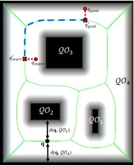
An example of a simple map with its corresponding GVD (green lines) is shown in Figure

3.1.

d(q,𝒬𝒪) q

𝒬𝒪

d(q,𝒬𝒪)

𝒬𝒪

𝒬𝒪 𝑞 𝑎

𝑞𝑔𝑜𝑎𝑙

𝑞′𝑎

𝑞𝑔𝑜𝑎𝑙′

Figure 3.1: An input image, corresponding GVD which is formed by green lines. The

black shapes show the obstacles (O) and the remaining space is free space (Qf ree).

Letqstart be a start configuration andqgoal be a target configuration. Let alsoQf ree be

the free configuration space. As any roadmap (RM), the GVD has three main properties as follows (Choset, 2005):

• Accessibility: there exists a path between any qstart∈ Qf ree and some q′start∈RM.

• Departability: there exists a path from some point on the RM,q′

goal ∈ RM, to

qgoal ∈ Qf ree .

• Connectivity: there exists a path in RM between q′

start and q

′

goal .

The GVD can be used as a safe route (since it maximizes distance between obstacles) to

connect any two configurations in the free space. This can be done easily by enforcing the robot to move from an initial configuration qstart to a point in the GVD, q′start, finding a

route to the point q′

goal also in the GVD and finally guiding the robot from q

′

goal to the

(26)

3.2.1 GVD Construction

There are several techniques to compute a GVD. For example, in a discrete grid, Brushfire (Choset, 2005) and wavefront (Zelinsky et al., 1993) are two useful methods.

In this work, the environment map (2D) is considered as an image, therefore in order to create the GVD on this image, a morphological approach is used. Morphological operators include a set of operators such as Dilation, Thinning, Skeletonization, Erosion and so on (Gonzalez and Woods, 2001). Usually the combination of these operators are used to give

different outputs. But before creating the GVD, it is necessary to compute free configu-ration space (Qf ree), where the robot can move freely without colliding with obstacles.

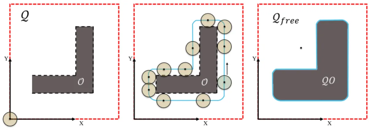
The common solution for computing the free configuration space is to construct the con-figuration space obstacle, QO. This is done by growing the obstacles by the size of the robot. As an example Figure 3.2(left) shows a two-dimensional workspace, Q, includes an obstacle, O. Also the result of growing a polygonal obstacle by the size of a circular robot is depicted in this figure (middle and right). After computingQO,Qf ree is given by:

Qf ree=Q\(S_iQOi).

It should be mentioned that circular robot in the workspace is equivalent to a point robot in the configuration space.

X Y

𝒪

X Y

𝒪

X Y

𝒬𝑂

𝒬

𝑟

𝒬

Figure 3.2: Result of the growth of a polygonal obstacle by the size of a circular robot.

Since the map is represented as an image, in our work in order to compute (Qf ree), we

use dilation operator to grow obstacles with size of the robot. In dilation, the structuring element has a vital role in the result. The robot shape is considered as the structuring element to compute the free configuration space (Qf ree). In this work a circular robot is

(27)

Figure 3.3: Disk shape robot.

Before representing more example of the dilation operator on an input map with circular structure element, a definition of the dilation operator is explained as following:

Suppose A is a binary image and B is the structural element. Dilation of A by B is defined as:

A⊕B ={x|(Bˆ)_x∩A6=∅}. (3.5) The basic effect of the dilation operator on a binary image is to gradually enlarge the boundaries of regions, which is applicable to computeQO.

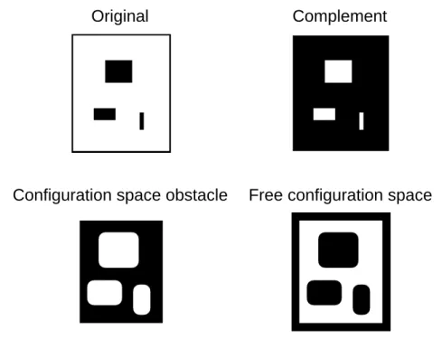
As it can be seen in figure 3.4, in the “original” image, the black regions show obstacles. The image “complement” or negative is computed to be used as the input of dilation operation. In the “configuration space obstacle” image, the white region represents the configuration space obstacle (QO) where robot collides with obstacle. By complementing

this image the final result of “free configuration space” is achieved, where the robot can freely move in the map, without having collision with obstacles.

Original Complement

Configuration space obstacle Free configuration space

(28)

Afterward, skeletonization operator is used to construct the GVD from Qf ree. The

informal definition of a skeleton is a line representation of an image that is one pixel thick, through the “middle” of the image, and preserves the topology of the image. Figure 3.5 shows the skeletons for the polygonal image. As can be seen, different size of disk is

used to create circular structuring element, therefore the result of skeleton are different respectively. More information about this operator can be find in (Gonzalez and Woods, 2001).

Figure 3.5: The white lines represent skeleton of the image.

Given the above explanation, skeletonization operator is applied to find the skeletal of the map which is demonstrated to be the GVD (Garrido et al., 2011). The Pseudo code of making the GVD is shown below:

Algorithm 2: GVD maker

Input: M,R // where M is input map and R contains robot shape and size

Output: GV D

1 M2 = Complement Image(M)

2 M3 = Dilate image(M2,R);

3 M4 = Complement Image(M3)

4 GVD = Image Skeleton(M4)

Figure 3.6 shows the results obtained from skeletonization techniques of the given map. In this figure, the junction of obstacles and the shaded area represent configuration

(29)

(a) Input map (b) GVD demonstration

Figure 3.6: The green lines are the skeleton of the map (GV D).

3.3 GVD Induced Graph

A graph G={V, E, C} is induced from the GVD by considering Meet Points (where

more than 2 GVD curves meet each other) or End Points (where curves terminates) as graph nodes and curves as graph edges. The set of vertices (nodes) is given by V, the set of edges by E ⊆ V ×V , and a cost function is denoted by C : E → R. The cost represents the distance between two vertices.

In Figure 3.7 the corresponding graph of the map in Figure 3.6 is illustrated.

6

3 ₂

4

5 7 8 9

10

𝑒 𝑒 𝑒

𝑒 𝑒

𝑒

𝑒 𝑒

𝑒

12

11

(30)

3.4 Multi-Objective Optimization

A multi-objective optimization problem involves multiple objective functions subject to a set of constraints. Such a problem can be described in mathematical terms as follows:

min(f1(x), f2(x), ....fm(x))

s.t, x∈S

(3.6)

where x∈ _Rn _{is a vector of variables,} _f

i(·) : Rn 7→ R are scalar functions, m > 1 is the

number of objectives, and S represents the set of feasible solutions, which is defined by the satisfaction of the problem constraints:

S={x∈Rn _:_h

j(x) = 0, gk(x)≥0}

In contrast to the single objective problem, the scalar concept of “optimality” does not apply directly in the multi-objective setting. In fact, instead of a scalar value solution, there exists a set of so-called Pareto optimal solutions. Decision making methods are

needed to select one of the solutions in the Pareto set.

Different interactive and evolutionary based algorithms have been proposed to solve multi-objective problems (Branke et al., 2008). An interesting multi-multi-objective evolutionary al-gorithm (MOEAs) is the Non Dominated Sorting Genetic Alal-gorithm II (NSGA-II) (Deb

and Pratap, 2002). As its name is evident, this algorithm has two parts: the first part is related to the use of non-domination rules and the second part is related to sorting a genetic population according to different preferred levels.

Domination will happen if a solution is better than the other in at least one objective and

equals in other objectives. Mathematically,

f(s1)≺f(s2),

where f() is a vector function f = [f1, f2, ..., fn]Tand s1, s2 ∈ S, which is the parameter space. In this case: fi(s1)≤fi(s2) ,∀i and fj(s1)< fj(s2) for at least one index j.

If the solutions do not dominate each other, we say that they are non-dominated or in-comparable.

(31)

disadvantages are the high computational complexity of non-dominated sorting and the lack of elitism.

NSGA-II is an improved version of NSGA and in this version, the disadvantages of NSGA is improved. Therefore, we used NSGA-II in this work.

3.4.1 Multi-objective Problem

As previously mentioned, in the present work, a robot must search for a specific object

on the map. The main problem here is that we assume we cannot wait for the complete search of the given environment. Therefore, our solution is to compute a finite number of good view points in the environment and then move the robot through these points in order to find the desired object. We define the multi-objective problem to define where

the SP sshould be placed. We consider the following objectives:

1. First objective: maximum covered area from the SPs.

As a first objective, we try to maximize the area of the map viewed by the sensors. As a result, since the object can be anywhere in the free environment, the probability of finding the object is maximized in this objective. We assume the robot is equipped

with sensors and is able to move so that the sensor footprint can be modeled by a circle centered at the robot position with radius r (see Figure 1.1).

(a) In contrast to SPi, in SPj

the robot has a maximum visi-ble range.

(b) SPs _{i, j, k} _{have less}

over-lap (Higher F2 value) thanSPs l, m, n.

Figure 3.8: A representation of objective functions on the map.

(32)

visible range is determined by the area viewed by the sensor after subtracting the portion occupied and occluded by obstacles (see Figure. 3.8 (a)). The first objective is given by:

F1 =

n

X

i=1

A(SPi), (3.7)

where n is the number of SPs and SPi ∈ GV D. A(SPi) is the covered area from

SPi i.e, it is the visible range. This objective function must be maximized.

Since the GVD is the set of points that maximizes the distance from obstacles it is interesting to note that by constraining the feasible set to this one dimensional set,

this not only reduces the dimension of the search space, but also helps in the visible range maximization and provides safety in the robot motion.

2. Second objective: good distribution of search points.

Overlapping is also another problem to be avoided when defining the positions of the

SPs in order to provide efficiency in the search. Thus, we require that the distance betweenSPs be maximized. In order to deal with this problem, we define the second objective as follows:

F2 =

n−1

X

i=1

n

X

j=i+1

kSPi−SPj k. (3.8)

In the equation above, F2 is the sum of Euclidean distances between all pairs

of SP s. Likewise the first objective, our second objective function (F2) must be maximized. According to the definition of good distribution, SP s i,j,k are better distributed than l,m,n in Figure 3.8.(b). In fact, the second objective aims to pro-vide a more uniform distribution of points over the map which is useful to avoid

sensor footprint overlaps.

3.4.2 Multi-objective Solution

(33)

Termination

criteria?

Initial random population

Non-domination sort

Yes

End

Genetic operation

Selection

No

Figure 3.9: Flowchart of NSGA II algorithm.

In the following, we show some details. a)Representation

Each chromosome contains a set ofSP s, and each gene refers to a position on the GVD,

pi ∈GV D. The table below illustrates the chromosome representation.

p1 p2 ... pn F1 F2 Table 3.1: Chromosome representation.

In Table 3.1,F1 andF2 are the values of the objective functions andnis the maximum number of points in the chromosome.

b) Initialization

(34)

Figure 3.10: Red points represent random SPs.

c)Evaluation and non-dominated sorting

Each chromosome is evaluated by computing its objective functions. Then, non-dominated sort ranks chromosomes based on their objectives. In addition the crowding distance is computed. The crowding distance is relative to the closeness of each individual to its

neighbor (Deb and Pratap, 2002). d) Operators

Genetic operators are usually applied to generate children. Genetic algorithm includes two basic operators: Crossover and Mutation.

In this work, we used two point crossover, in order to create new children from inheriting and merging the properties of two parents. This is illustrated in Figure 3.11.

Paretnt 1

Paretnt 2

Children2 Children1

Figure 3.11: Two point crossover.

An example of two point crossover operator is depicted in Figure 3.12, where two random parents are selected and after applying the crossover two new children are created.

(35)

(a) Two random parents.

(b) Two created children after operating crossover.

Figure 3.12: An example of crossover. Uncovered area has changed (decreased) in the new generation.

Different versions of mutation operator have been proposed for different situations. Here, in order to have a good exploration through the map, one gene is selected randomly

and it is replaced by a new random pointSP_{. This operator guarantees the variety of new} generation.

e) Selection

Before selection, the parent population and children concatenate together and they are

(36)

3.4.3 ELECTRE I

Choosing one solution over the set of solutions is also a challenge in MOEAs. In order to solve this challenge, decision making techniques are usually applied. ELECTRE

I is the multi-criteria decision making method applied to choose the best solution in our work (Shanian and Savadogo, 2006). The Elimination and Choice Translating Reality (ELECTRE) method was first introduced in (Shanian and Savadogo, 2006). It is one of the most extensively used outranking methods reflecting the decision makers preferences

in many fields. The ELECTRE I approach was then developed by a number of variants (Bojkovi´c et al., 2010).

This method is used to rank a set of alternatives and also to analyze the data of a deci-sion matrix (Shanian and Savadogo, 2006). This method is based on comparisons pairs

of all alternatives, which has lead to the make a partial ordering of options according to preference of decision maker.The method to form the final rankings uses two matri-ces:concordance matrix and discordance matrix.

In concordance matrix, values calculated for each pair of criteria that inform the extent

to which one alternative is at least as good as the other;

In discordance matrix, values calculated for each pair of criteria that inform the extent to which one alternative is worse than the other.

At the end, we define the relationship between the alternatives. We create a ranking

based on the difference amount of alternatives that exceeds alternative, and those that exceed it. Ranks the difference from the highest to the lowest.

3.5 Chinese Postman Problem

As previously mentioned, in our solution the robot must visit the search points to find the desired object. Therefore, it should be clear the necessity of efficiently solving this routing problem. In this work, we are going to use an algorithm that solve the so-called

Chinese Postman Problem.

Meigu Guan(or Kwan Mei-Ko), was a Chinese mathematician who proposed the Chinese postman problem(CPP) (Eiselt et al., 1995). Guan was interested in finding out how a postman could cover assigned segments at least once with minimum walking distance.

(37)

In the case of an undirected connected graph, a necessary and sufficient condition for an Euler cycle to exist is that the graph contains no node of odd degree. Such a graph is calledEulerian graph (Pearson and Bryant, 2004). Given an Eulerian graph, it is possible to find an Euler cycle in linear time by using the Hierholzer’s algorithm (Fleischner, 1991).

In the general case of non Eulerian graph, optimal routes for the Chinese Postman Problem can be found with complexityO(N3_{), where}_N _{is the number of nodes. The algorithm in} this case consists of finding the nodes of odd degree, finding a minimum length pairwise matching of the odd-degree nodes, adding to the graph the new edges of the shortest

paths between the two nodes in each of the pairs given by the minimum length pairwise matching, and finally finding the Euler tour in the modified graph which is now Eulerian (Larson and Odoni, 1981).

A common way to formulate the CPP is to seek a least-cost augmentation of G into G′

such that all nodes of G′ have an even degree. Consider xij as the number of repeat of

(vi, vj) required to add to G and let T ⊆V be the set of odd nodes ofV and define δ(i)

as the set of edges incident to vi. The formulation is as follow (Eiselt et al., 1995):

M inimize X

(vi,vj)∈A

cijxij, (3.9)

subject to

X

(vi,vj)∈δ(i)

xij ≡







1 (mod 2) if vi ∈T

0 (mod 2) if vi ∈V\T

(3.10)

xij ∈0,1((vi, vj)∈A) (3.11)

(38)

Algorithm 3: Chinese postman algorithm (Pearson and Bryant, 2004) Input: G// G is the graph

Output: Q //shortest closed route

1 Find and list all odd vertices in G.

2 Find and list all possible pairings of odd vertices (from step 1).

3 Find an edge for each pairing that connect the vertices with the minimum weight.

4 Find the pairings such that the sum of the weights is minimized.

5 On the input graph G add the edges that have been found in step 4. // The

length of an optimal chinese postman route is the sum of all the edges added to

the total found in step 4.

6 A route Q corresponding to this minimum weight can be found with Fleury ’s

algorithm.

After building the new graph, the Fleury ’s algorithm (Flurt, 1883) may find an Eulerian cycle which is the optimal solution for the CPP.

Fleury ’s algorithm is a method which, if followed, is guaranteed to produce anEulerian tour in a connected graph with no vertices of odd degree. In a connected graph, a bridge is defined as an edge which, if picked up, a disconnected graph is generated. (See Algorithm4)

Algorithm 4: Fleury’s Algorithm for finding an Eulerian tour (Wilson and Watkins, 1990)

Input: G// where Gis an Eulerian graph.

Output: //current trail is an Eulerian trail.

1 Select an arbitrary vertexv_i of G;

setcurrent vertex={vi};current trail={}.

2 cnt=1 // cnt is counter for edge number(edgenum).

3 while (cnt≤edgenum) do

4 Choose any edge (v_i, v_j) incident at v_i of current vertex which is not bridge unless there is no alternative.

5 Add (v_i, v_j) to the current trail;

cnt =cnt+ 1;

set the current vertex={vj};

6 Remove (v_i, v_j) from the graph; Remove any isolated vertices.

After Initialization, while loop repeats until all edges have been deleted from G. The final current trail is an Eulerian trail in G.

(39)

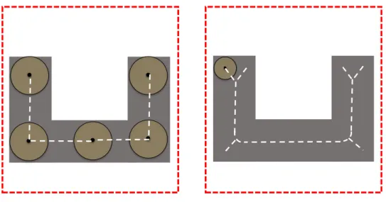
on this graph , a possible result can be as follows: 1 3 a b c g f 4 2 e d

(a) A graph with 4 nodes.

1 a b c g f 4 e d 2 3 c f

(b) Adding two virtual edges to two odd nodes.

Figure 3.13: Postman problem example.

Q={a, e, f, f, b, c, d, g, c},

where,Q includes a sequence of edges that indicates the Eulerian cycle.

3.6 Speeded Up Robust Features Algorithm

Object recognition is also an important problem in robotics. Hence applications of

mobile robots require not only the ability to move around in the environment and avoid obstacles, but also the ability to detect and recognize objects and interact with them. Most object recognizer/detector methods are based on two terms: training images and query images. Training images are the images which the detector uses to learn information.

Query images are the images from which the detector, after learning, is supposed to detect object(s). In this work, we want to use a robust object recognition method to be invariant in terms of scale and rotation. It means when the object in query image is at a different size or angle from the training images, the method can still recognize the object.

The Speeded Up Robust Features, in short (SURF) is a robust object recognition method that is a scale- and rotation invariant detector and descriptor (Bay et al., 2008). The SURF algorithm is mainly divided into three phases (Huijuan and Qiong, 2011): interest point detection, interest point descriptor and interest point matching. The main motivation of

(40)

phases of SURF algorithm.

• Interest point detection: In this phase SURF algorithm finds points which are in a special position in image such as corners, blob or spot and T-junction. The most valuable feature of interest point detection is repeatability which represents the reliability of detector in terms of finding same physical interest points in different viewpoints. In order to detect the interest points in image, the algorithm uses

Hessian matrix approximation because of its good performance in accuracy (Bay et al., 2008).

Suppose x=(x, y) is a point in image I, the Hessian matrix H(σ, x) in x at scale σ

is defined as follows:

H(σ, x)=





Lxx(σ, x) Lxy(σ, x)

Lxy(σ, x) Lyy(σ, x)



,

where Lxx(σ, x) is the convolution of the Gaussian second order derivative with the

image I in point x, and similarly for Lxy(σ, x) andLyy(σ, x).

• Interest point descriptor: This phase is divided in two steps: The first step consists in determining the orientation of interest points. Then in second step, descriptor uses Haar wavelets in a suitably oriented square region around the interest points to find intensity gradients in the X and Y directions. As the square region is divided into 16 squares for this, and each such sub-square yields 4 features, the

SURF descriptor for every interest point is 64 dimensional.

(41)

4 Simulation and Experimental

Results

In this section, first we show the two maps considered for our tests and also the corre-sponding GVD. Second we show the multi-objective solution to find theSPs. Simulation on ROS stage is presented in section 4.3. Next, we show how SURF algorithm could

rec-ognize the object in different tests. Finally, an experiment with a real robot is presented to validate the method.

4.1 Computing the GVD

As explained before, in order to create the GVD on input image, we used morpholog-ical operators such as dilation, skeletonization. We consider two different maps, a simple one and a more complex map (see Figure 4.1). As it can be seen, the corresponding GVD

(42)

(a) A simple map. (b) A complex map.

Figure 4.1: Two scenarios with their corresponding GVD.

4.2 Multi-Objective Solution in MATLAB

Our solutions were found using MATLAB on a computer with 4 GB RAM and CPU Core i 7.

In our simulation, we set the population size or chromosome number to 30. The dimension of each chromosome for simple map and complex map are respectively 16 and 60. It is

significant to mention that the dimension of chromosomes or the number of SPs is related to the maximum sensor range. In other words, when this range (r) is small, the number ofSPs should be large to cover the map. We defined a robot equipped with a laser sensor with maximum range equal to 10 meters (r= 10).

In each generation, 50% of the population is selected as elitism. The crossover probability,

Pc, is a noticeable parameter in this test and it is set to 70% (mutation ratio or Pm is

equal to 30%). Pm is high because the only way of generating new points along the GVD.

And also the maximum number of iterations is equal to 50. In order to use ELECTRE I,

(43)

4.2.1 Simulation Results:

This section presents one of the initial populations, which is generated randomly in a simple map. In Figure 4.2.(a) , theSPs were not well distributed and there are overlaps. Figure 4.2.(b) shows that a big area could not be covered by the robot. Hence, if the object is placed in this big area, the robot can not find it.

(a) Initial population. (b) Uncovered area from initial popula-tion is highlighted in gray color.

Figure 4.2: Initial population, its covered and uncovered region.

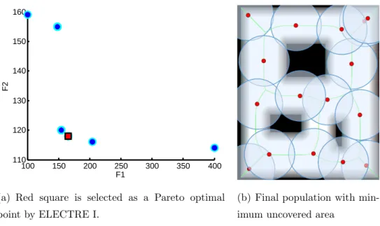
After running the NSGA-II on the simple map, a non-dominated set is obtained. In order to select one of the solutions, ELECTRE I is applied as our decision making tool. The non-dominated set and selected solution by using this technique are presented in Figure 4.3.(a). Because of the overlaps between solutions, just six solutions (out of 15

(44)

100 150 200 250 300 350 400 110 120 130 140 150 160 F1 F2

(a) Red square is selected as a Pareto optimal point by ELECTRE I.

(b) Final population with min-imum uncovered area

Figure 4.3: Result of multi-objective optimization for the simple map.

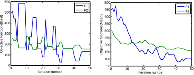
Figure 4.4.(a) presents the cost of objective functionsF1 and F2 with respect to iter-ation number. At each iteriter-ation, the values of objective functions for the best solution are

selected. This best solution is selected based on ELECTRE I. Figure 4.4.(b) also shows the mean values of objective functions in each iteration. Both plot indicate the progress of the algorithm in minimizing the objectives during iterations.

0 10 20 30 40 50

100 150 200 250 300 350 400 Iteration number Objective functions(Best) F1 F2

(a) The values of objective functions for best solution with respect to iteration number.

0 10 20 30 40 50

100 150 200 250 300 350 400 Iteration number Objective functions(Mean) F1 F2

(b) The mean values of objective functions with re-spect to iteration number.

Figure 4.4: The value of objective functions in iterations.

(45)

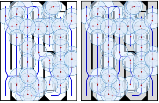
(a) Initial population. (b) Uncovered area from initial popula-tion is highlighted in gray color.

Figure 4.5: Initial population, its covered and uncovered region.

40 60 80 100 120 140 155

160 165 170 175 180 185

F1

F2

(a) Red square is selected as a Pareto optimal point by ELECTRE I.

(b) Final population with minimum un-covered area

(46)

0 10 20 30 40 50 0 100 200 300 400 500 600 Iteration number Objective functions(Best) F1 F2

(a) The values of objective functions for best solution with respect to iteration number.

0 10 20 30 40 50

50 100 150 200 250 300 350 400 450 500 Iteration number Objective functions(Mean) F1 F2

(b) The mean values of objective functions with re-spect to iteration number.

Figure 4.7: The value of objective functions in iterations.

4.3 Simulation on ROS/Stage

The Robot Operating System (ROS) (Quigley et al., 2009) is a framework to help in the development of robotic software. It consists of tools, libraries, and conventions that

aim to simplify the task of creating complex and robust robot behavior. Stage ROS is a useful package which allows for 2D robotic simulation. In order to verify the proposed exploration strategy, we tested it first on Stage ROS. This is an important step before implementing in the real robot to verify if the code is running as expected. In section 4.5

we show experiments with a real robot.

We defined a robot equipped with a laser sensor with maximum range equal to 10 meters (r = 10). The robot starts exploration in a random position in the map and move according to the route found by CPP in order to visit theSPs computed by the NSGA II with the help of ELECTRE I. At eachSP the robot captures data from the laser scanner to detect the object.

(47)

(a) Initial configuration (b) Object is found.

Figure 4.8: Snapshots of the exploration. Red points show theSPs on the GVD, yellow points show the points which have been explored so far by the robot.

4.4 Object Recognition with SURF

(48)

(a) Frame 1 (b) Frame 2 (c) Frame 3 (d) Frame 4

(e) Frame 5 (f) Frame 6 (g) Frame 7 (h) Frame 8

(i) Frame 9 (j) Frame 10 (k) Frame 11 (l) Frame 12

Figure 4.9: Training image set.

The screenshots below (see Figure 4.10) are the results of the tests that we performed using SURF. As it can be seen, there are three windows in the screenshot. The one on the left-up is the image representing the object of interest, that is, the object that we want the robot to find. The window on the center is an actual picture of the lab where the

(49)

(a) (b)

(c) (d)

Figure 4.10: The matched results of the SURF method.

4.5 Real Robot Results

The proposed method has been tested in a realistic scenario using the Pioneer plat-form1 _{shown in Figure 4.11. The name of this service robot is Maria and it is equipped} with all the necessary sensors for navigation and object recognition such as laser scanner

and Kinect.

(50)

Kinect

Laptop

Laser Scanner

Robot Platform

Figure 4.11: The structure of Maria and its sensors.

In our experiment, mapping and localization was provided by ROS packages. In order

to control the robot ’s linear and angular velocitiesv andw, respectively, so that the robot moves along the edges of the GVD, we used a static feedback linearization scheme (Desai et al., 1998). A real map of part of a building floor is considered for this experiment (see Figure 4.12.(a)). The size of this environment is 79.89×4.04meters. A predefined object

is placed in the map and the robot must find this object in minimum time. The initial configuration for the robot and also the position of the object are shown in Figure 4.12(a). The task of object recognition was done by using the local feature detection named Speed Up Robust Features (SURF) which is robust to rotation, scaling and affine transformation

(51)

(a) Input map, red square: robot initial configuration, green circle: position of the object.

1 1 2 2 3 3 4 4

5 5 6 6

7 7 8 8

9 9

10 10

11

11 1212

(b) Corresponding graph.

(c) Corresponding GVD andSPs_.

Figure 4.12: Input map, GVD and search points.

After constructing the GVD and the graph, we used NSGA II and ELECTRE I to find good locations for SPs. In Figures 4.12.(b) and (c), the graph and the distribution of SPs over the GVD are depicted, respectively.

Figure 4.13 shows the sequence of SP s visited by the robot. The object has been found

(52)

(a) Robot at 1th _SP_. _{(b) Robot at 5}th_SP_.

(c) Robot at 8th_SP_. _{(d) Robot at 10}th _SP_.

Figure 4.13: The sequence of visiting SPs.

Figure 4.14 represents the GVD and the trajectory executed by the robot according to the Chinese Postman Problem solution. The robot stopped exploration when the object

was found. A video of this experiment can be found in https://youtu.be/TC3TJDoX2C4/.

(53)

5 Statistical Analysis and

Comparison of Strategies

In the case of large maps in which a large number of search points is required, the use of our proposed automatic approach to distribute these points is clear when compared to

a normal distribution of points since the latter is unfeasible in such a scenario. However, in order to verify if the method is comparable or even better than an intuitive distribution of points done by a human specialist, we present in this chapter a comparison between the automatic proposed distribution and the manual distribution in the case of the small

maps previously shown.

In fact, this chapter focuses on the comparison of our proposed method with two other methods based on hypothesis testing. Before comparison of strategies, we give an example to describe some basic statistical concepts.

Consider our exploration problem described in the introduction. Suppose that we are interested in the time to find the object as a random variable that can be described by a probability distribution. Suppose that our interest focuses on the mean time to find the object (a parameter of this distribution). Specifically, we are interested in deciding

whether or not the mean time to find is 50 time units. We may express this formally as:







H0 :µ1 = 50

H1 :µ1 6= 50

(5.1)

The statement H0 : µ1 = 50 time units in above equation is called the null hypothesis.

This is a claim that is initially assumed to be true. The statement H1 : µ1 6= 50 time units is called the alternative hypothesis and it is a statement that contradicts the null hypothesis. Testing the hypothesis involves taking a random sample, computing a test statistic from the sample data, and then using the test statistic to make a decision about

(54)

¯

x is observed. The sample mean is an estimate of the true population mean µ. Suppose that if 48.5 ≤ x¯ ≤ 51.5, we will not reject the null hypothesis H0 : µ1 = 50, and if either ¯x < 48.5 or ¯x > 51.5, we will reject the null hypothesis in favor of the alternative hypothesisH1 :µ1 6= 50. This is illustrated in Figure 5.1.

µ=50 µ=51.5

µ=48.5

α/2 α/2

Acceptance region

Critical region Critical region

Fail to reject H0

Reject H0 Reject H0

Figure 5.1: Decision criteria for testing H0 :µ1 = 50 versus H1 :µ1 6= 50.

The acceptance region is a region where all values of ¯x are in the interval 48.5≤x¯≤

51.5 and we will fail to reject the null hypothesis; The values of ¯xthat are less than 48.5 and greater than 51.5 constitute the critical region for the test. We reject H0 if the test statistic falls in the critical region and fail to reject H0 otherwise.

This decision procedure for testing null hypothesis can lead to two wrong conclusions (Campelo, 2014): type I error and type II error.

Type I erroris rejection of the null hypothesis H0 when it is true.

The probability of occurrence of type I error is calledsignificance level (α):

α=P(type I error) = P(reject H0|H0 is true) (5.2)

The selected value of α defines the critical threshold for the rejection of H0. In our ex-ample (see Figure 5.1), a type I error will occur when either ¯x < 48.5 or ¯x > 51.5 when

(55)

Failing to reject the null hypothesis when it is false is defined as a type II error. The probability of occurrence of atype II error in any test of hypotheses is generally repre-sented byβ:

β =P(type II error) = P(f ail to rejectH0|H0 is f alse) (5.3)

The quantity (1−β) is known aspower of the test, and quantifies its sensitivity to effects that violate the null hypothesis.

5.1 Comparison of First and Second Strategies in

Robot Exploration Experiment with Simple Map

To compare two strategies statistically, we divided the necessary tasks in four steps as follows: problem description, experimental design, analysis of experiment, and discussion and conclusion.

5.1.1 Problem Description

In this part, we compare the average time to find (TTF) the object of our strategy (S1) with another strategy(S2) which will be explained below. More specifically, we are

interested in knowing whether mean TTF measured by each strategy differs by more than 10 time units asminimally interesting difference.

In this section strategy (S1) refers to our proposed method where the robot moves along the GVD and execute the search at theSPs. In this strategy allSPs are found by NSGA II. On the other hand, in second strategy(S2), robot explores the created GVD of input map and stops at specific points namelySPs to find the object similary to S1. However there is a constraint inS2 such that every graph edge of GVD has at least oneSP placed on it.

In this experiments, the input map is the simple one in Figure 3.6(b) In order to have available information, experiments are performed to generate initial data for the two strategies. It means that the two different strategies (S1, S2) are run to save elapsed time

for finding the object. For this reason, the object positions is changed 20 times for each strategy.

The result is considered relevant when it can generate effects greater than the minimally interesting difference(δ) of 10 time units. The other desired characteristics for the

(56)

• Significance level(α): 0.1

• Power level(1−β): 0.8

The selected value of significance level defines the critical threshold for the rejection of

H0 and the power level of the test quantifies its sensitivity to effects that violate the null hypothesis.

5.1.2 Experimental Design

In this subsection, we divided the design of experiment in three parts as follows:

first, we illustrated how to construct statistical hypothesis testing . In the next part we describe the results of an experiment with a linear statistical model. Lastly we determine the sample size required for hypothesis testing.

5.1.2.1 Statistical Hypothesis

The experimental design is primarily defined by the establishment of the null and alternative hypotheses, H0 and H1 respectively. Consider robot exploration experiment introduced earlier, we may think that the mean of TTF in S1 is equal to mean of TTF

inS2. This may be stated formally as equation below:







H0 :µ1 =µ2

H1 :µ1 6=µ2

(5.4)

whereµ1 is the mean of TTF inS1 andµ2 is the mean of TTF in S2. The null hypothesis is that the mean of TTF inS1 (µ1) is equal to mean of TTF in S2 (µ2) and alternate is that µ1 is different from µ2.

5.1.2.2 Representation of Observations

(57)

the data from our experiment is (Montgomery and Runger, 2013):

yij =µi+ǫij







i= 1,2

j = 1, .., ni

(5.5)

where yij is the jth observation of ith strategy; µi is the mean of each strategy; And ǫij

stands for the residual associated withith strategy at thejth observation.

5.1.2.3 Choice of Sample Size

An important part of any experimental design is determining appropriate sample sizes (Montgomery, 2012); We need to determine how many observations are enough in order to draw conclusions about a population using a sample from that population. That

is deciding the number of replicates to run. Choice of sample size depends on some parameters such as: minimally interesting effect (δ) or true difference between means , standard deviation(sd), significance level(α) and power of test.

To perform statistical tests, there is a high level programming language for data analysis

and graphics which is called “R”. This language includes various functions in statistics area,mathematics, graphics and etc that is used as statistical computing tools (Crawley, 2012).

We used a powerful command in R implementation which can be used to compute sample

size considering target power. The command is known as power.t.test(...). To compute the required sample size, we need to have the necessary parameters which are mentioned above and also know about type of t.test which is two.sample and type of alternative that is two.sided.

Since the variance is not known and it is essential for computing sample size, it will be estimated from the data. As we are assumingσ2

1 ≈σ22, we can use the pooled variance Sp2

(Montgomery, 2012):

S_p2 = (sd12+sd22)/2 (5.6)

where sd1 and sd2 are the standard deviation of two sample data (S1,S2). As a result,

Sp equals to 36.

Multi-objective approach for robot exploration

Title:

Multi-Objective Approach for Robot

Exploration

Kossar Jeddisaravi

Multi-Objective Approach for Robot

Exploration

Kossar Jeddisaravi

Abstract

Contents

List of Figures

List of Tables

List of Symbols

List of Abbreviations

1

Introduction

1.1

Motivation

1.2

Objectives

1.3

Thesis Organization

2

Literature Review

3

Methodology

3.1

Proposed Method

3.2

Generalized Voronoi Diagram

3.2.1

GVD Construction

𝒬

𝒬

3.3

GVD Induced Graph

3.4

Multi-Objective Optimization

3.4.1

Multi-objective Problem

3.4.2

Multi-objective Solution

Termination

criteria?

Initial random population

Non-domination sort

Non-domination sort

Yes

End

Genetic operation

Selection

3.4.3

ELECTRE I

3.5

Chinese Postman Problem

3.6

Speeded Up Robust Features Algorithm

4

Simulation and Experimental

Results

4.1

Computing the GVD

4.2

Multi-Objective Solution in MATLAB

4.2.1

Simulation Results:

4.3

Simulation on ROS/Stage

4.4

Object Recognition with SURF

4.5

Real Robot Results

5

Statistical Analysis and

Comparison of Strategies

5.1

Comparison of First and Second Strategies in

Robot Exploration Experiment with Simple Map

5.1.1

Problem Description