On a Gradient Flow of Plane Curves Minimizing
the Anisoperimetric Ratio
Daniel ˇSevˇcoviˇc and Shigetoshi Yazaki
Abstract—We analyze a gradient flow of closed planar curves minimizing the anisoperimetric ratio. For such a flow the normal velocity is a function of the anisotropic curvature and it also depends on the total interfacial energy and enclosed area of the curve. In contrast to the gradient flow for the isoperimetric ratio, we show there exist initial curves for which the enclosed area is decreasing with respect to time. We also derive a mixed anisoperimetric inequality for the product of total interfacial energies corresponding to different anisotropy functions. Finally, we present several computational examples illustrating theoretical results.
Index Terms—Anisoperimetric ratio, gradient geometric flows, mixed anisoperimetric ratio inequality, tangential sta-bilization
I. INTRODUCTION
T
HE goal of this paper is to investigate a geometric flow of closed plane curvesΓt, t≥0, minimizing theanisoperimetric ratio. We will show that the normal velocity
β for such a geometric flow is a function of the anisotropic curvature, the total interfacial energy and enclosed area of an evolved curve,
β=δ(ν)k+FΓ, (1)
wherekis the curvature andδ(ν)>0is a strictly positive co-efficient depending on the tangent angleν at a pointx∈Γt.
HereFΓ is a nonlocal part of the normal velocity depending
on the entire shape of the curveΓ = Γt and the termδ(ν)k
represents the anisotropic curvature. In typical situations, the nonlocal part is a function of the enclosed area A and the interfacial energyLσ=RΓσds, i.e.FΓ=F(A, Lσ). As an
example one can consider
β =k−2Lπ,
whereL≡L1is the length of an evolved closed curveΓ. It
is well known that such a flow represents the area preserv-ing geometric evolution of closed embedded plane curves investigated by Gage [8]. Among other geometric flows with nonlocal normal velocity we mention the curvature driven length preserving flow in whichβ=k−21π
R
Γk2dsstudied
by Ma and Zhu [16] and the inverse curvature driven flow preserving the length β = −k−1 + L
2π studied by Pan
and Yang [21]. The isoperimetric ratio gradient flow with
β = k−L/(2A) has been proposed and investigated by
Manuscript received April 27, 2013; revised June 6, 2013. This work was supported in part by the VEGA grant 1/0747/12 (DS) and Grant-in-Aid for Scientific Research (C) 23540150 (SY)
Prof. D. ˇSevˇcoviˇc, PhD., is with the Department of Applied Mathematics and Statistics, Comenius University, 842 48 Bratislava, Slovak Republic. e-mail: [email protected]
Prof. S. Yazaki, PhD., is with the Department of Mathematics, School of Science and Technology, Meiji University, Kanagawa 214-8571, Japan. email: [email protected]
Jiang and Zhu [14] for convex curves and by the authors in [23] for general closed Jordan curves evolving in the plane. Recently, a classical nonlocal curvature flow preserving the enclosed area was reinvestigated by Xiao et al. in [25]. They proved uniform upper bound and lower bound on the curvature. Furthermore, Mao et al. [17] showed that such a nonlocal flow will decrease the perimeter of the evolving curve and make the curve more and more circular during the evolution process. Applying inequalities of Andrews and Green-Osher type, Lin and Tsai [15] showed that the evolving curves will converge to a round circle, provided that the curvature is a-priori bounded. However, most of those fine results for area preserving flow still have to be extended to the case of a class of non-local flows minimizing the isoperimetric and/or anisoperimetric ratio.
The main goal of this paper is twofold. First we derive the normal velocityβ corresponding to the anisoperimetric ratio gradient flow. It turns out thatβ =kσ−Lσ/(2A)wherekσis
the anisotropic curvature, i.e.βhas the form of (1). We derive and analyze several important properties of such a geometric flow. In contrast to the isoperimetric ratio gradient flow (c.f. Jiang and Zhu [14], [23]), we show that the anisoperimetric ratio gradient flow may initially increase the total length and, conversely, decrease the enclosed area of evolved curves. In order to verify such striking phenomena, an accurate numerical discretization scheme for fine approximation of the geometric flow has to be proposed. This is the second principal goal of the paper. We derive a numerical scheme based on the method of flowing finite volumes with combi-nation of asymptotically uniform tangential redistribution of grid points. The idea of a uniform tangential redistribution has been proposed by How et al in [13] and further analyzed by Mikula and ˇSevˇcoviˇc in [18]. The asymptotically uniform tangential redistribution has been analyzed in [20], [19]. The scheme is tested on the area-decrease and length-increase phenomena as well as on various other examples of evolution of initial curves having large variations in the curvature.
anisotropy functions. In section 6 we investigate properties of the enclosed area for the anisoperimetric gradient flow. In contrast to a gradient flow for the isoperimetric ratio, we will show that there are initial convex curves for which the enclosed area is strictly decreasing. Finally, in section 7 we construct a counterexample to a comparison principle showing that there initial noninteresting curves such that they intersect each other immediately when evolved in the normal direction by the anisoperimetric ratio gradient flow. In section 8 we derive a numerical scheme for solving curvature driven flows with normal velocity depending on no-local terms. The scheme is based on a flowing finite volume method combined with a precise scheme for approximation of non-local terms. We present several numerical examples illustrating theoretical results and interesting phenomena for the gradient flow for anisoperimetric ratio.
II. SYSTEM OF GOVERNING EQUATIONS AND CURVATURE ADJUSTED TANGENTIAL REDISTRIBUTION
In this section we recall description and basic properties of geometric evolution of a closed plane Jordan curveΓwhich can be parameterized by a smooth functionx: [0,1]→R2
such that Γ = Image(x) ={x(u); u∈[0,1]} and|∂ux|>
0. We identify the interval [0,1] with the quotient space
R/Zby imposing periodic boundary conditions forx(u)at
u= 0,1. We denote∂ξF=∂F/∂ξ, and|a|=√a·awhere
a·bis the Euclidean inner product between vectorsaandb. The unit tangent vector is given byT =∂ux/|∂ux|=∂sx,
where s is the arc-length parameter ds = |∂ux|du. The
unit inward normal vector is defined in such a way that
det(T,N) = 1. Then the signed curvaturekin the direction
N is given byk= det(∂sx, ∂s2x). Letν be a tangent angle,
i.e., T = (cosν,sinν)T and N = (−sinν,cosν)T. From
the Fren´et formulae ∂sT = kN and ∂sN = −kT we
deduce that∂sν=k.
Geometric evolution problem can be formulated as fol-lows: for a given initial curveΓ0= Image(x0) = Γ, find a
family of curve{Γt}
t≥0,Γt={x(u, t); u∈[0,1]}starting
fromΓ0and evolving in the normal direction with the
veloc-ityβ. In this paper we follow the so-called direct approach in which evolution of the position vector x = x(u, t) is governed by the equation:
∂tx=βN +αT, x(·,0) =x0(·). (2)
Here α is the tangential component of the velocity vector. Note that α has no effect on the shape of evolving closed curves, and the shape is determined by the value of the normal velocityβ only. Therefore, one can take take α≡0
when analyzing analytical properties of the geometric flow driven by (2). On the other hand, the impact of a suitable choice of a tangential velocity αon construction of robust and stable numerical schemes has been pointed out by many authors (see [22], [23] and references therein).
In what follows, we shall assume that β = δ(ν)k+FΓ
where δ(ν) > 0 is a strictly positive 2π-periodic smooth function of the tangent angle ν and FΓ is a nonlocal part of the normal velocity depending on the entire shape of the curve Γ. According to [19] (see also [18], [20]) the system of PDEs governing evolution of plane curves evolving in the normal and tangential directions with velocitiesβ andα
reads as follows:
∂tk=∂s2β+α∂sk+k2β, (3)
∂tν =∂sβ+αk, (4)
∂tg= (−kβ+∂sα)g, (5)
∂tx=δ(ν)∂s2x+α∂sx+FΓN, (6)
foru∈[0,1]andt >0. Hereg=|∂ux|is the so-called local
length (c.f. [18]). A solution to (3)–(6) is subject to periodic boundary conditions forg, k,xatu= 0,1,ν(0, t)≡ν(1, t)
mod(2π) and the initial condition k(·,0) =k0(·), ν(·,0) =
ν0(·), g(·,0) = g0(·),x(·,0) = x0(·) corresponding to the
initial curveΓ0= Image(x0).
Local existence and continuation of a classical smooth solution to system (3)–(6) has been investigated by the authors in [22], [23]. In this paper we therefore take for granted that classical solutions to (3)–(6) exists on some maximal time interval[0, Tmax)(c.f. [23], [20]).
III. THEWULFF SHAPE AND INTERFACIAL ENERGY FUNCTIONAL
The anisotropic curvature driven flow of embedded closed plane curves is associated with the so-called interfacial energy density (anisotropy) function σ defined on Γ. It is assumed that σ = σ(ν) is a strictly positive function depending on the tangent angle ν only. With this notation we can introduce the total interfacial energy
Lσ(Γ) = Z
Γ
σ(ν) ds
associated with a given anisotropy density functionσ. Ifσ≡ 1thenL1(Γ)is just the total length L(Γ)of a curveΓ. The
Wulff shape is defined as an intersection of hyperplanes:
Wσ= \
ν∈S1
x= (x1, x2)T; −x·N ≤σ(ν)
.
If the boundary∂Wσ of the Wulff shape is smooth and it
is parameterized by∂Wσ ={x=−σ(ν)N +a(ν)T, ν ∈
[0,2π]}, then, it follows from the relation ∂sν=k that
T =∂sx= (−σ′(ν) +a(ν))kN + (σ(ν) +a′(ν))kT.
Hencea(ν) =σ′(ν)and(σ(ν) +σ′′(ν))k= 1holds and the
boundary∂Wσ can be parameterized as follows:
∂Wσ={x; x=−σ(ν)N +σ′(ν)T, ν ∈[0,2π]},
and its curvature is given by k = (σ(ν) +σ′′(ν))−1. Let
us denote bykσ the anisotropic curvature defined by kσ :=
(σ(ν) +σ′′(ν))k. It means that the anisotropic curvaturek
σ
of the boundary∂Wσ of the Wulff shape Wσ is constant, kσ ≡1. Moreover, the area |Wσ| =A(∂Wσ)of the Wulff
shape satisfies:
|Wσ| = −
1 2
Z
∂Wσ
x·Nds= 1 2
Z
∂Wσ
σ(ν) ds
= 1
2Lσ(∂Wσ).
Clearly, |W1| = π for the case σ ≡ 1. If we consider the
2,3,· · ·, ε(m2−1)<1 then the area ofWσ can be easily
calculated:
|Wσ| =
1 2
Z
∂Wσ
σ(ν) ds=1 2
Z 2π
0
σ(σ′′+σ)dν
= π
2(2−ε 2(m2
−1)). (7)
In Fig 1 we plot shapes of ∂Wσ for various degreesm.
m= 2 m= 3 m= 4
m= 5 m= 6
Fig. 1. The Wulff shapesWσform= 2,· · ·,6andε= 0.99/(m 2
−1).
Since the global quantities evaluated over the closed curve
Γ do not depend on the tangential velocity α we may take α ≡ 0. Hence ∂tg = −kβg and ∂tν = ∂sβ. These
identities follow from (4) and (5) with α ≡0. Recall that
∂sν =k. Therefore∂sσ′(ν) = σ′′(ν)∂sν =σ′′(ν)k and so R
Γσ
′′(ν)kds= 0. Hence
Z
Γ
kσds= Z
Γ
σkds
holds. For the time derivative ofRΓkσdswe obtain
d dt
Z
Γ
kσds=
d dt
Z 1
0
σkgdu=
Z 1
0
[∂t(σk)g+σk∂tg]du
=
Z
Γ
[∂t(σk)−σk2β]ds
=
Z
Γ
[k∂tσ(ν) +σ(ν)∂tk−σ(ν)k2β]ds
=
Z
Γ
[kσ′(ν)∂
tν+σ(ν)(∂tk−k2β)]ds
=
Z
Γ
[kσ′(ν)∂
sβ+σ(ν)∂s2β]ds= 0,
because∂tk−k2β =∂2sβandkσ′(ν) =σ′(ν)∂sν=∂sσ(ν).
From the previous equality we can deduce the following identity:
Z
Γt
kσds= Z
Γ0
kσds, for any 0≤t < Tmax, (8)
where the family of planar embedded closed curves Γt, t∈
[0, Tmax), evolves in the normal direction with the velocity β.
Now, let us consider an evolving family of plane embedded closed curves Γt, t ∈ [0, T], homotopicaly connecting a
given curve Γ = Γ0 and the boundary ΓT = ∂W
σ of the
Wulff shape Wσ. The homotopy can be realized by taking
a suitable normal velocityβ (eventually depending on the position vectorx). Using such a normal velocity we deduce the identity:
Z
Γ
kσds= Z
∂Wσ
kσds=L(∂Wσ). (9)
It means thatRΓkσdsis equal to the length of the boundary ∂Wσ of the Wulff shape. The same result has been recently
obtained by Barrett et al. in [2, Lemma 2.1]. We can say that identity (9) is a generalization of the rotation number:
1 2π
R
Γkds= 1, since2π=L(∂W1).
Remark 1: Identity (9) can be easily shown for convex
curves. Indeed, if Γ is convex then its arc-length param-eterization s can be reparameterized by the tangent angle
ν ∈ [0,2π]. We have ∂sν = k > 0 and therefore
ds=k−1dν. Hence
Z
Γ
kσds= Z
Γ
σkds=
Z 2π
0
σ(ν)dν.
For the lengthL(∂Wσ)of the boundary of a convex Wulff
shape we obtain
L(∂Wσ) = Z
∂Wσ ds=
Z 2π
0 1 kdν
=
Z 2π
0
[σ(ν) +σ′′(ν)]dν =
Z 2π
0
σ(ν)dν.
ThereforeRΓkσds=L(∂Wσ) because R2π
0 σ
′′(ν)dν = 0
andk= [σ(ν)+σ′′(ν)]−1on∂W
σ. IfΓis not convex we can
apply the famous Grayson’s theorem [12]. We let it evolve according to the normal velocityβ =k until a time t=T
whenΓT becomes convex. Using (8) and previous argument
we again obtain identity (9).
Let us denote by L1 the total interfacial energy
corre-sponding to σ≡1, i.e. L1 ≡L. Let Γ =∂W1 be the unit
circle. Then, by applying identity (9), we deduce
L1(∂Wσ) =Lσ(∂W1). (10)
Latter identity can be rephrased as follows: the length of the boundary∂Wσ of the Wulff shape equals to the total
inter-facial energy of the unit circle. It can be easily generalized to the case of arbitrary two anisotropiesσ(ν)andµ(ν). We have the following proposition:
Theorem 1: Letσ andµbe two smooth anisotropy
func-tions satisfyingσ(ν) +σ′′(ν)>0, µ(ν) +µ′′(ν)>0. Then
the duality
Lµ(∂Wσ) =Lσ(∂Wµ) (11)
between total interfacial energies of boundaries ∂Wσ and ∂Wµ of Wulff shapes holds.
P r o o f. Notice that the Wulff shapes Wσ and Wµ are
convex sets becauseσ(ν)+σ′′(ν)>0andµ(ν)+µ′′(ν)>0
k= [σ(ν) +σ′′(ν)]−1 and so
Lµ(∂Wσ) = Z
∂Wσ
µ(ν)ds (12)
=
Z 2π
0
µ(ν)1 kdν =
Z 2π
0
µ(ν)(σ(ν) +σ′′(ν))dν
=
Z 2π
0
[µ(ν)σ(ν)−σ′(ν)µ′(ν)]dν=Lσ(∂Wµ),
(13)
arguing vice versa. ♦
IV. GRADIENT FLOW FOR THE ANISOPERIMETRIC RATIO.
Recall that for the enclosed areaA=A(Γt)and the total
length L = L(Γt) for a flow of embedded closed plane
curves driven in normal direction by the velocityβ we have
d dtA+
Z
Γt
βds= 0, d dtL+
Z
Γt
kβds= 0, (14)
(c.f. [18]). Using governing equations (3)–(6), for the total interfacial energyLσ=Lσ(Γt)of a curveΓt, we obtain
d dtLσ=
d dt
Z
Γ
σ(ν)ds= d dt
Z 1
0
σ(ν)gdu (15)
=
Z 1
0
[σ′(ν)∂
tνg+σ(ν)∂tg]du
=
Z
Γ
[σ′(ν)∂sβ−σ(ν)kβ]ds (16)
=−
Z
Γ [σ′′(ν)∂
sνβ+σ(ν)kβ]ds (17)
=−
Z
Γ
[σ′′(ν) +σ(ν)]kβds= −
Z
Γ
kσβds.
Here we have used the governing equations (5) and (4) (with
α ≡ 0) and the identity ∂sν = k. For the anisoperimetric
ratio
Πσ(Γ) =
Lσ(Γ)2
4|Wσ|A(Γ) ,
we have Πσ(Γ)≥1 and, in particular, Πσ(∂Wσ) = 1 (see
Remark 3). Taking into account identities (15) and (14) we obtain
d
dtΠσ =
Lσ∂tLσ
2|Wσ|A − L2
σ∂tA
4|Wσ|A2
= −2 Lσ |Wσ|A
Z
Γ
kσ−
Lσ
2A
βds.
Hence, the flow driven in the normal direction by the non-locally dependent velocity
β =kσ− Lσ
2A (18)
represents a gradient flow for the anisoperimetric ratio Πσ
with the property∂tΠσ<0forβ6≡0. Notice thatβ≡0on
Γif and only ifΓ∝∂Wσ, i.e.Γis homotheticaly similar to ∂Wσ.
In the caseσ≡1the isoperimetric ratio gradient flow has been analyzed by Jiang and Zhu in [14] and by the authors in [22]. In this case the normal velocity has the form: β = k−L/(2A).
V. AMIXED ANISOPERIMETRIC INEQUALITY
The aim of this section is to prove a mixed anisoperimetric inequality of the form
Lσ(Γ)Lµ(Γ)
A(Γ) ≥Kσ,µ, (19)
which holds for any C2 smooth Jordan curve Γ in the
plane. Here Kσ,µ>0 is a constant depending only on the
anisotropy functions σ and µ such that σ(ν) +σ′′(ν)> 0
and µ(ν) +µ′′(ν) > 0 hold for any ν. The existence of
a minimizer of the mixed anisoperimetric ratio is discussed in Remark 2. The idea of the proof of the inequality (19) is rather simple and consists in solving the constrained minimization problem:
min
Γ Lσ(Γ), s.t. Lµ(Γ) =cA(Γ), (20)
wherec >0is a given constant. To this end, let us assume that a curve Γ = Γ(x) is parameterized by a C2 smooth
function x : S1 → R2. If we denote g ≡ g(x) = |∂
ux|
the local length then, for the derivative ofg in the direction
y:S1 →R2, we obtain 2g(x)g′(x)y= 2(∂
ux·∂uy) and
so
g′(
x)y= (T·∂sy)g. (21)
Here and here after, for scalar-valued function f(x) and vector-valued functionf(x) = (f1(x), f2(x))T we denote
their derivatives in the directiony by
f′(x)y:=∇f(x)·y= lim
ε→0
f(x+εy)−f(x)
ε ,
f′(x)y:=
f′
1(x)y
f′ 2(x)y
,
respectively.
As for the tangent vector T = T(x) = (cosν,sinν)T
we have T(x) = g−1∂
ux and so T′(x)y = g−1∂uy − g−2∂
uxg′(x)y = ∂sy−(T ·∂sy)T = (N ·∂sy)N. As
N = (−sinν,cosν)T, for the derivative of the tangent angle
ν=ν(x), we obtain
ν′(
x)y=N·∂sy. (22)
Recall that kσ := (σ(ν) +σ′′(ν))k and ∂sν = k. Since Lσ(Γ) =
R
Γσds=
R1
0 σ(ν)gduwe obtain
L′
σ(Γ(x))y= Z 1
0
[σ′(ν)ν′(
x)yg+σ(ν)g′( x)y] du
=
Z
Γ
[σ′(ν)(N·∂sy) +σ(ν)(T ·∂sy)] ds
=−
Z
Γ
[σ′′(ν)∂
sν(N·y)−σ′(ν)k(T ·y)
+σ′(ν)∂
sν(T·y) +σ(ν)k(N·y)] ds
=−
Z
Γ
[σ(ν) +σ′′(ν)]k(
N·y)ds
=−
Z
Γ
kσ(N·y)ds.
Hence
L′
σ(Γ(x))y = − Z
Γ
kσ(N ·y)ds,
L′
µ(Γ(x))y = − Z
Γ
For the areaA=A(Γ)enclosed by a Jordan curveΓ = Γ(x)
we haveA= 1 2
R1
0 det(x, ∂ux)du. Therefore
A′(Γ(
x))y= 1 2
Z 1
0
det(y, ∂ux) + det(x, ∂uy)du
=
Z 1
0
det(y, ∂ux)du= Z
Γ
det(y,T)ds.
Since det(y,T) =−y·N we obtain
A′(Γ(x))y=−
Z
Γ
N ·yds. (24)
In order to solve the constrained minimization problem (20) we introduce the Lagrange functionL(x, λ) =Lσ(Γ(x)) + λ(Lµ(Γ(x))−cA(Γ(x))) withλ >0.
Then the first order condition for Γ = Γ( ¯¯ x) to be a minimizer of (20) reads as follows: 0 = L′x(x, λ)y
≡
L′
σ(Γ(x))y + λ(L′µ(Γ(x))y −cA′(Γ(x))y) at x = ¯x.
Latter equality has to be satisfied for any smooth function
y:S1→R2. Taking into account (23) and (24) we obtain
kσ+λkµ =λc, on Γ¯.
It means that
kσ¯=λc, on Γ¯, where σ¯=σ+λµ. (25)
In other words,Γ =¯ 1
λc∂Wσ¯(up to an affine translation in the
planeR2). The Lagrange multiplierλ∈Rcan be computed from the constraintLµ(¯Γ) =cA(¯Γ). It follows from duality
(11) (see Proposition 1) that
Lµ(∂Wσ¯) = Lσ¯(∂Wµ) =Lσ(∂Wµ) +λLµ(∂Wµ)
= Lσ(∂Wµ) + 2λA(∂Wµ).
To calculate the enclosed area A(¯Γ) = 1
λ2c2A(∂Wσ¯) we
make use of the identityA(∂W¯σ) =12Lσ¯(∂W¯σ). Clearly, as
¯
σ=σ+λµwe obtain
Lσ¯(∂Wσ¯) =Lσ(∂Wσ¯) +λLµ(∂Wσ¯) =Lσ¯(∂Wσ) +λL¯σ(∂Wµ)
=Lσ(∂Wσ) +λLµ(∂Wσ) +λLσ(∂Wµ)
+λ2Lµ(∂Wµ)
= 2A(∂Wσ) + 2λLσ(∂Wµ) + 2λ2A(∂Wµ).
Since λc1Lµ(∂Wσ¯) = Lµ(¯Γ) = cA(¯Γ) = λ2cc2A(∂Wσ¯)we
end up with the identity
1
λc(Lσ(∂Wµ) + 2λA(∂Wµ))
= c
λ2c2 A(∂Wσ) +λLσ(∂Wµ) +λ 2A(∂W
µ)
.
Since the Lagrange multiplier λ > 0 it is given by λ=
p
A(∂Wσ)/A(∂Wµ). Furthermore,
Lσ(∂Wσ¯) = Lσ¯(∂Wσ) =Lσ(∂Wσ) +λLµ(∂Wσ)
= 2A(∂Wσ) +λLσ(∂Wµ).
Now, letΓbe an arbitraryC2smooth Jordan curve in the
plane. Setc=Lµ(Γ)/A(Γ). Then
Lσ(Γ)Lµ(Γ)
A(Γ) =cLσ(Γ)≥cLσ(¯Γ) = c
λcLσ(∂Wσ¯)
= 2
q
A(∂Wσ)A(∂Wµ) +Lσ(∂Wµ).
Remark 2: The proof of existence of a minimizer of the
mixed anisoperimetric ratioLσ(Γ)Lµ(Γ)/A(Γ)is as follows:
letΓn= Γ(xn)be a sequence of Jordan curves minimizing
this ratio. As Lσ(γΓ) = γLσ(Γ), and A(γΓ) = γ2A(Γ)
for eachγ > 0, without lost of generality, we may assume
L(Γn) = 1 for all n ∈ N. We can also fix the barycenter
of Γn at the origin. Since c
0L(Γ) ≤ Lσ(Γ) ≤ c1L(Γ)
where 0 < c0 = minΓσ ≤ c1 = maxΓσ < ∞, then,
by the isoperimetric inequality, the value of the infimum is positive. Moreover, the parameterization xn of Γn can
be chosen in such a way that |∂uxn| = L(Γn) = 1. As
a consequence, the position vectors {xn(u), u ∈ [0,1]}
are uniformly bounded. By the Arzel`a-Ascoli theorem there is a convergent subsequence converging to some function
{x(u), u ∈ [0,1]} which is the minimizer of the mixed anisoperimetric ratio.
In summary, we have shown the following mixed anisoperimetric inequality:
Theorem 2: Let Γ be a C2 smooth Jordan curve in the
plane. Then
Lσ(Γ)Lµ(Γ)
A(Γ) ≥Kσ,µ, (26)
where Kσ,µ = 2 p
|Wσ||Wµ|+Lσ(∂Wµ).The equality in
(26) holds if and only if the curveΓis homothetically similar to the boundary∂Weσ of a Wulff shape corresponding to the
mixed anisotropy functionσe=p|Wµ|σ+ p
|Wσ|µ.
Remark 3: If σ = µ ≡ 1 we obtain the well known
isoperimetric inequality L(Γ)2/A(Γ) ≥ K
1,1 ≡ 2 √
π2 +
L(W1) = 4π. If σ = µ we obtain the anisoperimetric
inequalityLσ(Γ)2/A(Γ)≥Kσ,σ= 2 p
|Wσ|2+Lσ(∂Wσ) =
4|Wσ|. Finally, ifµ≡1we obtain the mixed anisoperimetric
inequality
Lσ(Γ)L(Γ)
A(Γ) ≥Kσ,1≡2
p
π|Wσ|+L(∂Wσ).
Remark 4: In the caseµ=σ, the anisoperimetric inequal-ity in the plane has been stated in a paper by G. Wulff [24] from 1901. Later, it was proved by Dinghas in [4] for a special class of polytopes. Recently, Fonseca and M¨uller [5] proved the anisotropic inequality in the plane. Later Fusco
et al. [6] proved it in arbitrary dimension. Giga in [10]
pointed out that the anisotropic inequality where µ = σ
are π-periodic function is the isoperimetric inequality in a suitable Minkowski metric. It is a useful tool in the proof of anisotropic version of the so-called Gage’s inequality (c.f. [9, Corollary 4.3]).
However, in all aforementioned proofs, the surface energy was associated with a functionalLΦ(Γ) =RΓΦ(N)dswhere Φ :R2→Ris an absolute homogeneous anisotropy function of degree one, i.e.Φ(tx) =|t|Φ(x)for any t∈R,x∈R2. The relation between our description of anisotropy and the latter one is: σ(ν) = Φ(−sinν,cosν) and, conversely,
Φ(x) = σ(ν) where x/kxk = (−sinν,cosν). Since we do not require π-periodicity of σ, in our approach of de-scription of anisotropy we therefore allow for non-symmetric anisotropies, like e.g. functions σ with odd degree m (see Fig 1) corresponding thus to anisotropy function Φ which are positive homogeneous only, i.e.Φ(tx) =tΦ(x)for any
In the case of general anisotropy functions µ 6≡ σ, the mixed anisoperimetric inequality derived in Theorem 2 is, to our best knowledge, new even in the case of symmetric (π-periodic) anisotropy functions.
VI. CONVEXITY PRESERVATION. TEMPORAL AREA AND LENGTH BEHAVIOR
In this section we analyze behavior of the enclosed area
A(Γt)of a curveΓt evolved in the normal direction by the
anisoperimetric ratio gradient flow, i.e.β=kσ−Lσ/(2A).
First we prove the preservation of convexity result stating that the anisoperimetric ratio gradient flow preserves con-vexity of evolved curves. In the case of the isoperimetric ratio gradient flow of convex curves with β=k−L/(2A), the convexity preservation has been shown by Jiang and Pan in [14]. However, similarly as Mu and Zhu in [16], they utilized the Gauss parameterization of the curvature equation (3) by the tangent angle ν and this is why their results are applicable to evolution of convex curves only. In our paper we first prove convexity preservation based on the analysis of the curvature equation (3) with arc-length parameterization. Moreover, we show the anisoperimetric ratio gradient flow may initially increase the total length and decrease the enclosed area. This phenomenon cannot be found in the isoperimetric ratio gradient flow (c.f. [14], [22]).
Theorem 3: LetΓt, t∈[0, T
max), be the anisoperimetric
ratio gradient flow of smooth Jordan curves in the plane evolving in the normal direction by the velocityβ=kσ−L2Aσ.
If the curveΓt0 is convex at some timet
0∈[0, Tmax)then
Γtremains convex for anyt∈[t
0, Tmax).
P r o o f. Since ∂tk=∂s2β+k2β,∂tν =∂sβ =∂skσ and β =kσ+FΓ we have
∂tkσ=δ(ν)∂tk+δ′(ν)k∂tν
=δ(ν)∂s2kσ+δ(ν)k2β+δ′(ν)k∂skσ
=δ(ν)∂s2kσ+
1 δ(ν)k
2
σβ+δ
′
(ν)k∂skσ,
whereδ(ν) :=σ(ν) +σ′′(ν)>0.
Let us denote by K(t) = minΓtk
σ(., t) the minimum of
the anisotropic curvature kσ = δ(ν)k over the curve Γt.
Denote by s∗(t)
∈[0, Lt] the argument of the minimum of kσ, i.e. K(t) = kσ(s∗(t), t). Then ∂skσ(s∗(t), t) = 0 and ∂2
skσ(s∗(t), t)≥0. Hence K′(t)
≥∆(1t)K(t)2(K(t) +Ft
Γ),
where∆(t) =δ(ν(s∗(t), t)), andFt
Γ=−Ltσ/(2At). Notice
that∆(t)≥∆min := minνδ(ν)>0 for all t ∈[0, Tmax).
Suppose that K is a solution to this ordinary differential inequality existing on some interval[t0, Tmax)and such that K(t0) >0. Then, it should be obvious that K(t) > 0 for
t∈[t0, Tmax)provided that
inf
t0≤t≤t∗F t
Γ >−∞, (27)
for every 0 < t∗ < T
max. In order to prove convexity
preservation for the anisoperimetric ratio gradient flow it is therefore sufficient to verify that the nonlocal part FΓt = −Lt
σ/(2At) remains bounded from below for t ≥ t0. To
prove boundedness of FΓt from below we utilize a property
of the anisoperimetric ratio. Indeed, as β =kσ−Lσ/(2A)
represents gradient flow for the anisoperimetric ratio Πt σ =
(Lt
σ)2/(4|Wσ|At) we have 1 ≤ Πtσ ≤ Π0σ for all t ∈
[0, Tmax). Thus
Ft
Γ=−
Lt σ
2At ≥ −
(L0
σ)2
2A0 1 Lt
σ .
Now, since the classical solution exists on the time interval
[0, Tmax) then inf0≤t≤t∗Ltσ > 0 for each 0 < t∗ < Tmax
and the estimate (27) follows. ♦
In what follows, we shall investigate the enclosed area and length behavior of curves evolved by the normal velocity
β=kσ−Lσ/(2A)representing thus a gradient flow for the
anisoperimetric ratio.
Using the area equation (14) we obtain
d
dtA = − Z
Γ
βds=−
Z
Γ
kσ−
Lσ
2A
ds
= −L(∂Wσ) + LLσ
2A . (28)
By applying the isoperimetric inequality (see Remark 3) for the case σ ≡ 1 and any curve Γ = Γt, the following
inequality:
d
dtA=−2π+ L(Γ)2 2A(Γ) ≥0
holds. It means that the gradient flow for the isoperimetric ratio does not decrease the enclosed area. On the other hand, if anisotropy density functionσ 6≡const, then for a curve
Γ = Γt∝∂W
¯
σ corresponding to the Wulff shapeWσ¯ with
the anisotropy functionσ¯ =√π σ+p|Wσ| we obtain
d
dtA = −L(∂Wσ) + LLσ
2A =−L(∂Wσ) + 1 2Kσ,1 = pπ|Wσ| −
1
2L(∂Wσ)<0 (29)
due to the isoperimetric inequality L(∂Wσ)2 ≥
4πA(∂Wσ) = 4π|Wσ|. It means that the gradient flow for
the anisoperimetric ratio may initially decrease the enclosed area for special initial curves.
Next we recall the isoperimetric inequality by Gage. According to [7] the following inequality holds:
Z
Γ
k2ds≥πL
A (30)
for any convexC2 smooth Jordan curve in the plane. The equality in (30) holds iffΓis a circle. Therefore, in the case of isoperimetric gradient flow with σ ≡ 1 and the convex curveΓt, we have
d dtL
t=
−
Z
kβds=−
Z
Γ
k2ds+πL
A ≤0. (31)
However, ifσ6≡const is a smooth nonconstant anisotropy density function such thatσ+σ′′>0, there exists an initial
curveΓ0 such that the lengthLt may initially increase, i.e.
d
dtLt>0 att= 0. Indeed, letΓ0 be an initial curve which
homothetically similar to the boundary ∂Wσ¯ of the Wulff
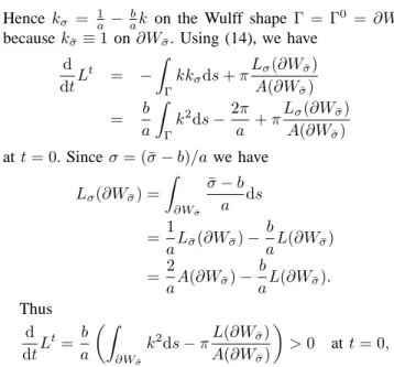
shape corresponding to the mixed anisotropy functionσ¯ = aσ+b wherea, b >0 are constants. Then
kσ=k¯σ−b a =
1 ak¯σ−
Hence kσ = 1a −abk on the Wulff shape Γ = Γ0 = ∂Wσ¯
becausek¯σ≡1 on∂Wσ¯. Using (14), we have d
dtL
t = −
Z
Γ
kkσds+π
Lσ(∂Wσ¯)
A(∂Wσ¯)
= b
a Z
Γ
k2ds−2aπ+πLσ(∂Wσ¯) A(∂Wσ¯)
att= 0. Sinceσ= (¯σ−b)/awe have
Lσ(∂Wσ¯) =
Z
∂W¯σ ¯ σ−b
a ds
= 1
aL¯σ(∂Wσ¯)− b
aL(∂Wσ¯)
= 2
aA(∂Wσ¯)− b
aL(∂Wσ¯).
Thus
d dtL
t= b a
Z
∂Wσ¯
k2ds−πL(∂W¯σ) A(∂W¯σ)
>0 att= 0,
due to inequality (30) and the fact that ∂Wσ¯ is a convex
curve different from a circle forσ¯6≡const.
In summary, we have shown the following result.
Theorem 4: Ifσ≡1then the isoperimetric ratio gradient
flow with the normal velocity β = k −L/(2A) is area nondecreasing and length nonincreasing flow of smooth Jordan curves Γt, t ∈ [0, T
max) in the plane provided that
Γ0is a convex curve.
Assume the anisotropy functionσis not constant and such thatσ+σ′′>0. LetΓ0be an initial curve which is
homoth-etically similar to the boundary∂Wσ¯ of a Wulff shape with
the modified anisotropy density function ¯σ=aσ+bwhere
a, b are constants, a, b > 0. Then, for the anisoperimetric ratio gradient flowΓt, t∈[0, T
max), evolving in the normal
direction by the velocityβ =kσ−L2Aσ, we have
1) ddtL(Γt)>0att= 0.
2) If, moreover,a/b=√π/p|Wσ| then ddtA(Γ
t)<0at t= 0.
VII. ACOUNTEREXAMPLE TO THE COMPARISON PRINCIPLE
The aim of this section is to demonstrate that the com-parison property does not hold under the anisoperimetric gradient flow, which is quite in a contrast to the total-length gradient flow β = k. It is a well-known fact that the comparison argument plays a key role in the proof of the famous Gage-Hamilton-Grayson theorem for the curvature driven flow β = k, and it states that two smooth curves, one of them included in the closure of the interior of the second one, evolved by the normal velocity β = k never intersects each other [11], [12]. The aim of this section is to show that the analogous comparison property does not hold for the anisoperimetric gradient flow. As the flow
β = kσ −Lσ/(2A) is nonlocal, violation of comparison
principle can be expected. Nevertheless, we provide an explicit construction of a counterexample in this section.
Clearly, any curve Γ homotheticaly similar to the Wulff shape ∂Wσ is a stationary curve, i.e. β ≡0 on Γ. Indeed, kσ ≡1 on ∂Wσ and F∂Wσ =−Lσ(∂Wσ)/(2A(∂Wσ)) =
−1and therefore β=kσ+F∂Wσ ≡0on∂Wσ.
In what follows, we shall construct a smooth initial curve
˜
Γ0containing in its interior the Wulff shape ∂W
σ and such
that Γ˜t intersects the stationary Wulff shape ∂W
σ for all
sufficiently small times 0 < t≪ 1. The construction is as follows. First, we shall construct a nonsmooth curveΓˆas the unionΓ =ˆ ∂Wσ∪r·∂W1 of the Wulff shape∂Wσ and the
circle r·∂W1 of a radiusr > 0 touching the Wulff shape
from outside at a pointy(see Fig 2 (left)). For such a curve we have
FΓˆ = −Lσ(ˆΓ) 2A(ˆΓ) =−
Lσ(∂Wσ) +Lσ(r·∂W1) 2(A(∂Wσ) +A(r·∂W1))
= −LσL(∂Wσ) +rLσ(∂W1)
σ(∂Wσ) + 2πr2
because A(∂Wσ) = Lσ(ˆΓ)/2. Hence FˆΓ > −1 provided
that the radius r is sufficiently large, r > Lσ(∂W1)/2π.
For instance, ifσ(ν) = 1 +εcos(mν), then r >1 because
Lσ(∂W1) = 2π(see section 3).
Let x˜0 ∈ Γˆ ∩∂Wσ be a point different from y and
belonging to a part of the curve representing the Wulff shape. Now, let us construct an initial smooth curve Γ˜0
which is a continuous perturbation of Γˆ, it contains the Wulff shape in the closure of its interior, and such that
˜
Γ0≡Γˆin some neighborhoodO( ˜x)ofx˜(see Fig 2 (right)).
The anisoperimetric ratio gradient flow Γ˜t, t ≥ 0, starting
from Γ˜0 intersects the stationary Wulff shape ∂W
σ in the
neighborhoodO( ˜x)for any time 0 < t≪1 (Γ˜t is plotted
by a dashed curve in Fig 2 (right)). This is a consequence of the fact that the normal velocityβ atx˜0 is strictly positive fort= 0 becauseβ=kσ+FΓ˜0= 1 +F˜Γ0 >0atx˜0, and
˜
Γ0∩ O( ˜x) =∂W
σ∩ O( ˜x), i.e. kσ= 1atx0.
WV w
1 r˜ wW
y
0 x
1
ˆ W r W
V
* w ‰ ˜ w
y
0 x
0 *
t *
t x
Fig. 2. An initial nonsmooth curveΓˆ (left) and its smooth perturbation
˜ Γ0
(right). Failure of a comparison principle occurs at the pointx˜0 and 0< t≪1.
VIII. NUMERICAL EXPERIMENTS
scheme with variational structure in a discrete sense. Their scheme has the second order of accuracy in time. However, discretized polygonal curves are restricted to a certain class of curves which is analogous to the admissible class in crystalline curvature flows or crystalline algorithm. In what follows, we propose a hybrid scheme taking into account advantages from both aforementioned schemes.
Discretization scheme. For a given initialN-sided polyg-onal curveP0=SNi=1S0
i, we will find a family ofN-sided
polygonal curves{Pj}j=1,2,···,Pj=SNi=1Sij, whereSij= [xji−1,xji]is thei-th edge withx0j =xjN forj= 0,1,2,· · ·. The initial polygonP0is an approximation ofΓ0 satisfying {x0
i}Ni=1 ⊂ P0∩Γ0, and Pj is an approximation of Γt at
the time t = tj, where tj = jτ is the j-th discrete time
(j = 0,1,2,· · ·) if we use a fixed time increment τ > 0, or tj =Pjl=0−1τl (j = 1,2,· · ·; t0 = 0) if we use adaptive
time incrementsτl>0, l= 0,· · ·, j−1. The updated curve
Pj+1is determined from the data forPjat the previous time
step by using discretization in space and time. Our two steps scheme will be constructed as follows: in the first step we construct moving polygonal curves which is continuous in time and discrete in space. In the second step we make use of the semi-implicit time discretization scheme for moving polygonal curves.
Step 1: Moving polygonal curves. LetP(t) =SNi=1Si(t)
be an N-sided polygonal curve continuously in time with
P(0) = P0, where Si(t) = [xi−1(t),xi(t)] is the i
-th edge and xi(t) is the i-th vertex (i = 1,2,· · ·, N;
x0(t) = xN(t)). The length of Si is denoted by ri =
|xi−xi−1|. Thei-th unit tangent vectorTi can be defined
as Ti = (xi−xi−1)/ri, and the i-th unit inward normal
vector Ni = Ti⊥, where (a, b)⊥ = (−b, a). Then the i-th
unit tangent angleνi is obtained fromTi = (cosνi,sinνi)T
in the following way: Firstly, from T1 = (T11, T12)T, we
obtain ν1 = −arccos(T11) if T12 < 0; ν1 = arccos(T11)
if T12 ≥0. Secondly, for i = 1,2,· · ·, N we successively
computeνi+1 fromνi:
νi+1=
νi−arccos(I), if D <0, νi+ arccos(I), if D >0, νi, otherwise,
whereD= det(Ti,Ti+1), I =Ti·Ti+1. Finally, we obtain
ν0=ν1−(νN+1−νN). Then the i-th unit inward normal
vector Ni isNi = (−sinνi,cosνi)T.
Let us introduce the “dual” volume S∗
i = [x∗i,xi] ∪
[xi,x∗i+1]ofSi, wherex∗i = (xi−1+xi)/2is the mid point
of the i-th edge Si (i = 1,2,· · ·, N; x∗N+1 = x∗1). The
length ofSi∗ isr∗
i = (ri+ri+1)/2. Then the total length of P is L=PNi=1ri =PNi=1r∗i, and the enclosed area ofP
isA=−PNi=1(xi·Ni)ri/2 =PNi=1x⊥i−1·xi/2.
We define thei-th unit tangent angle ofS∗
i byνi∗= (νi+ νi+1)/2 = νi+φi/2, where φi = νi+1−νi is the angle
between the adjacent two edges. Then thei-th tangent vector at the vertex xi is Ti∗ = (cosνi∗,sinνi∗)T and the inward
normal vector N∗
i = (−sinνi∗,cosνi∗)T. Hereafter we will
use the following abbreviations:
ci= cos φi
2, si= sin φi
2 (i= 1,2,· · · , N).
Then it is easy to check that
Ti∗=ciTi+siNi, Ni∗=ciNi−siTi (i= 1,2,· · · , N).
The evolution equations ofP(t)read as follows:
˙
xi=αiTi∗+βiNi∗ (i= 1,2,· · ·, N), (32)
where αi and βi are quantities defined on Si∗. Here and
hereafter, we denote u˙ = du/dt. The tangential velocities
{αi} are defined below and the i-th normal velocity βi is
defined such as
βi= β∗
i +βi∗+1 2ci
(i= 1,2,· · · , N), (33)
where thei-th normal velocityβ∗
i is defined onSi. It is an
approximation of (1) such as
β∗
i =δiki+FΓ (i= 1,2,· · ·, N).
Here ki is the i-th curvature and the constant value on Si
defined as
ki=
tan(φi/2) + tan(φi−1/2)
ri
(i= 1,2,· · · , N),
which is the same as the polygonal curvature in [3], andδi
is an approximation ofδ(νi)defined later. Then we obtain
the time evolution of the total length ofP(t):
˙ L=−2
N X
i=1
βisi=− N X
i=1
kiβi∗ri,
and the time evolution of the enclosed area ofP(t):
˙
A=−
N X
i=1
βicir∗i + N X
i=1
αisi
ri+1−ri
2 (34)
=−
N X
i=1
β∗
iri+ errA, (35)
errA=− N X
i=1
β∗
i
ri+1−2ri+ri−1
4 +
N X
i=1
αisi
ri+1−ri
2 .
These identities represent a discrete version of equations (14) provided that the distributionri ≡L/N, i= 1,2,· · ·, N,is
uniform because the error termerrA= 0 is vanishing.
To realize this uniform distribution asymptotically, we assume that
ri− L N =ηie
−f(t)
PN
i=1ηi = 0,f(t)→ ∞as t→Tmax≤ ∞
.
By using a relaxation termω(t) =f′(t)we obtain
˙ ri−
˙ L
N =
L N −ri
ω(t),
Z Tmax
0
ω(t) dt=∞ (36)
(i= 1,2,· · ·, N). Taking into account the relations:
˙
ri= ( ˙xi−x˙i−1)·Ti
=−βisi−βi−1si−1+ciαi−ci−1αi−1
= L˙
N +
L N −ri
ω(t),
we deduceN−1equations for tangential velocitiesαi(i=
2,3,· · ·, N):
αi=
Ψi ci
+c1 ci
α1 (i= 2,3,· · · , N),
Ψi=ψ2+ψ3+· · ·+ψi (i= 2,3,· · ·, N),
ψi=βisi+βi−1si−1− 2
N N X
i=1
βisi+
L N −ri
To determine α1, we add one more linear equation of the
form PNi=1αipi = P, which is independent of the above N−1 equations. Since
R=c1
N X
i=1
pi ci
, Q=
N X
i=2
pi ci
Ψi, (37)
we obtain α1 = (P −Q)/R. Next, we propose three
candidates for each {pi} and P, and choose one of them
in the following way:
Candidate 1. We put
pi=si
ri+1−ri
2 (i= 1,2,· · ·, N),
P =
N X
i=1
β∗i
ri+1−2ri+ri−1
4 ,
and from (37) we calculate Rand Q. We denote thisR by
R1. If the above equation holds, then errA = 0 and A˙ =
−PNi=1βi∗ri hold in (35). However, if distribution of grid
points are almost uniform, then the above equation is almost nothing. Therefore we need another candidate.
Candidate 2. For thei-th quantitiesFi defined onSi and Gi defined on S∗
i, we define the average alongP such as
hFi= 1
L N X
i=1
Firi, hGi∗= 1
L N X
i=1 Gir∗
i.
Since L = PNi=1ri =PNi=1r∗i, we have h1i= h1i∗ = 1.
Moreover, forα∗
i = (αi+αi−1)/2defined onSi, the relation
hαi∗=hα∗iholds.
The second candidate of linear equation is the zero-average
hαi∗ = 0, that is, p
i =r∗i fori= 1,2,· · ·, N andP = 0.
From this and (37) we calculateRandQ. We denote thisR
byR2.
The purpose of this section is to present numerical sim-ulations of the geometric flow evolving according to the evolution equation (18). Before we introduce the third can-didate, we calculate the discrete version of (18). Let the total interfacial energy be
Lσ(t) = N X
i=1
σ(νi(t))ri(t).
The time derivative ofTi = (cosνi,sinνi)T isT˙i = ˙νiNi.
Then we haveriν˙i = ( ˙xi−x˙i−1)·Ni, from which it follows
that
˙ Lσ =
N X
i=1 (σ′
iν˙iri+σir˙i) =− N X
i=1
kσ iβi∗ri+ N X
i=1
kσ ip˜iαi,
˜
pi= (σ′i+σi′+1)si+ (σi−σi+1)ci.
Hereσi=σ(νi),σi′ =σ′(νi), andkσ i is discrete version of
the weighted curvature in the following sense:
kσ i=δiki,
δi = σ′
i+1−σ′i−1 2(ti+ti−1) +
σi+1ti+σi(ti+ti−1) +σi−1ti−1 2(ti+ti−1) ,
ti = tan φi
2 ,
andδi is discrete weight ofδ(ν) =σ′′(ν) +σ(ν)atν =νi.
Note that δi → δ(νi) holds as φi, φi−1 →0 formally, and
even the case whereti+ti−1= 0,kσ iis well-defined, since ki = (ti+ti−1)/ri and then denominator ofkσ i is2ri.
We obtain d dt L2 σ A =
2Lσ A
˙ Lσ−
Lσ
2AA˙
,
˙ Lσ−
Lσ
2AA˙ =− N X
i=1
kσ i−
Lσ
2A
β∗
iri+ errratio,
errratio= N X
i=1 ˜ piαi
+Lσ 2A
XN
i=1
β∗
i
ri+1−2ri+ri−1 4
−
N X
i=1
αisi
ri+1−ri
2
.
Candidate 3. We put
pi=si
ri+1−ri
2 −
2A Lσ
˜
pi (i= 1,2,· · · , N),
P = N X i=1 β∗ i
ri+1−2ri+ri−1
4 ,
and from (37) we calculateR andQ. We denote thisR by
R3. Let thei-th normal velocity defined onSi be
β∗
i =kσ i− Lσ
2A (i= 1,2,· · ·, N),
which is discrete version of (18). If we choose the candidate 3 and its hold exactly, thenerrratio= 0holds and we obtain
d dt
L2
σ
A =−
2Lσ A
N X
i=1
kσ i−
Lσ
2A 2
ri<0.
Choice one from three candidates. We choose candidate
numberl satisfying
|Rl|= max{|R1|,|R2|,|R3|}.
Remark 5: If, for definition of the normal velocity defined
onS∗
i, we use
βi= β∗
iri+βi∗+1ri+1 2ciri∗
instead of (33), thenkσ i can not be divided into weighted
partwi and the curvatureki. Moreover, if we use
βi= β∗
i +β∗i+1 2
instead of (33), then kσ i can be divided into weighted part
and the curvature. However, we haveerrA6= 0, that isA˙ =
−PNi=1βi∗ridoes not hold even if uniform distributionri≡ L/N holds for all i= 1,2,· · · , N.
Step 2: Discretization in time. We use semi-implicit
scheme for discretization of (32). Next we develop expres-sion (32) as follows:
˙
xi = αiTi∗+βiNi∗
= 1
2
αi
ci − βisi
Ti+
1 2
αi ci
+βisi
Ti+1
+βici
Ni+Ni+1
2 (38)
= 1
2
αi
ci − βi si
Ti+
1 2
αi
ci
+βi si
Here we have used the relation
T∗
i =
Ti+1+Ti
2ci ,
Ni∗ = si
Ti+1−Ti
2 +ci
Ni+1+Ni
2 =
Ti+1−Ti
2si .
Letµbe a parameter satisfyingµ= 0ifmin1≤i≤N|si|= 0,
otherwiseµ∈(0,1]. For the parameterµ∈[0,1]we use the linear interpolation of (38) and (38), since we can not use (38) if si= 0.
Put bi = (1−µ)si+µ/si forµ∈(0,1]andbi=si for µ= 0. Then the evolution equation instead of (32) will be
˙ xi =
1 2
αi
ci − βibi
Ti+
1 2
αi
ci
+βibi
Ti+1
+βici(1−µ)
Ni+Ni+1
2 . (39)
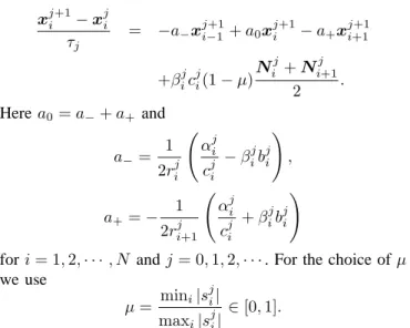
From Ti = (xi −xi−1)/ri, we discretize (39) in time
and obtain the following tridiagonal linear system under the periodic boundary condition:
xji+1−xji
τj
= −a−xji−1+1+a0xji+1−a+xji+1+1
+βijcji(1−µ)N
j i +N
j i+1
2 .
Herea0=a−+a+ and
a−= 1 2rij
αji cji −β
j ib
j i
! ,
a+=− 1 2rji+1
αji cji +β
j ib
j i
!
fori= 1,2,· · ·, N andj= 0,1,2,· · ·. For the choice ofµ
we use
µ= mini|s
j i|
maxi|sji|
∈[0,1].
Here and hereafter, mini and maxi mean min1≤i≤N and
max1≤i≤N, respectively. Note that maxi|sji|>0 holds for
closed curves.
In order to ensure solvability of the above linear system, we require a simple condition on the diagonal dominance. Adopting such a condition the adaptive time stepτj satisfies
τj =
minirji
2(1 +λ)(maxi|αji/c j
i|+ maxi|βjib j i|)
(λ >0).
Simulation. In following all figures, for the prescribedbτ > 0, we plot everyµbτ discrete time step using discrete points representing the evolving curve. In every3µbτ time step, we plot a polygonal curve connecting those points, whereµ= [[T /τb]/100]([x]is the integer part ofx), andT = 1.5is the final computational time. We useω≡1000as the relaxation term in (36). Note that if we use small ω, then asymptotic speed for uniform distribution becomes slow, and for some choice ofσarea-decreasing phenomena do not hold near the initial time (cf. Fig 4 (a)).
Wulff shapes and area-decreasing phenomenon. If σ(ν) = 1 +εcos(mν) is the anisotropy density function of the degree m then, by using (7), we obtain the explicit expression for the mixed anisotropy function:
¯
σ=√π σ+p|Wσ|
=√π 1 +εcosmν+
r
1−ε2m2−1 2
! .
In order to verify the area-decreasing and the length-increasing phenomenon at the initial time as in Theorem 4, we use ∂Wσ¯ as the initial curve. Fig 3 (a) indicates ∂Wσ¯
with m= 6. Its discretization is given by the uniform N -division of the u-range [0,1]. Fig 3 (b) indicates the same Wulff shape, but the grid points are distributed uniformly. Fig 3 (c) indicates the time evolution starting from (b).
(a) (b)
(c)
Fig. 3. (a) The Wulff shape∂W¯σwithN= 120points, (b) its uniform parameterization and its time evolution (c).
39.036 39.038 39.04 39.042 39.044 39.046
0 0.2 0.4 0.6 0.8 1 1.2 1.4 22.18 22.2 22.22 22.24 22.26 22.28 22.3 22.32
the enclosed area A the total length L
time area length
Fig. 4. Initial decrease of the enclosed areaAand increase of the total lengthL.
Although deformation of ∂Wσ¯ is very small (see
Fig 3 (c)), the area-decreasing and the length-increasing phenomenon can numerically verified by using the afore-mentioned numerical discretization scheme. The behavior of the enclosed area and total length of curves evolved from the initial Wulff shape∂Wσ¯ with the mixed anisotropy density
(a)
(b)
(c)
(d)
(e)
Fig. 5. Evolution of curves starting from the initial curves with various choice of peak ofσ.
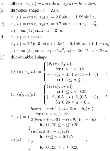
Initial test curves. As initial test examples we use the
boundary∂Wσ¯ of the Wulff shape as well as the following
initial curves x(u,0) = (x1(u), x2(u))T (u∈[0,1])
param-eterized by
(a) ellipse:x1(u) =acos 2πu, x2(u) =bsin 2πu, (b) dumbbell shape:z= 2πu,
x1(u) = cosz, x2(u) = 2.0 sinz−1.99 sin3z, (c) x1(u) = cosz, x2(u) = 0.7 sinz+ sinx1+x23,
x3= sin(3z) sinz, z = 2πu, (d) x1(u) = 1.5 cosz,
x2(u) = 1.5(0.6 sinz+ 0.5x23+ 0.4 sinx4+ 0.1 sinx5),
x3= sin(3z) sinz, x4= 2x12, x5= 3e−x1, z= 2πu, (e) thin-dumbbell shape:
(x1(u), x2(u)) =
(¯x1(u),x¯2(u))
for0≤u <0.5 −(¯x1(u−0.5),x¯2(u−0.5))
for0.5≤u≤1
,
(¯x1(u),x¯2(u)) =
(ˆx1(u),xˆ2(u))
for0≤u <0.25 (−ˆx1(0.5−u),xˆ2(0.5−u))
for0.25≤u≤0.5
,
ˆ x1(u) =
beam+rad(1 + cos(8(π−θε)u))
for0≤u <0.125
2(beam+rad(1−cosθε))(1−4u)
for0.125≤u≤0.25
,
ˆ x2(u) =
radsin(8(π−θε)u))
for0≤u <0.125 ε
for0.125≤u≤0.25 ,
where beam > 0 and 0 < ε < rad are parameters and
θε= arcsin(ε/rad).
In all examples, the initial discretization is given by the uniform N-division of the u-range [0,1]. Fig 5 indicates numerical simulation with the initial curves. We choose several peaks ofσsuch as (a)m= 2, (b)m= 3, (c)m= 4, (d)m= 5, and (e) m= 6.
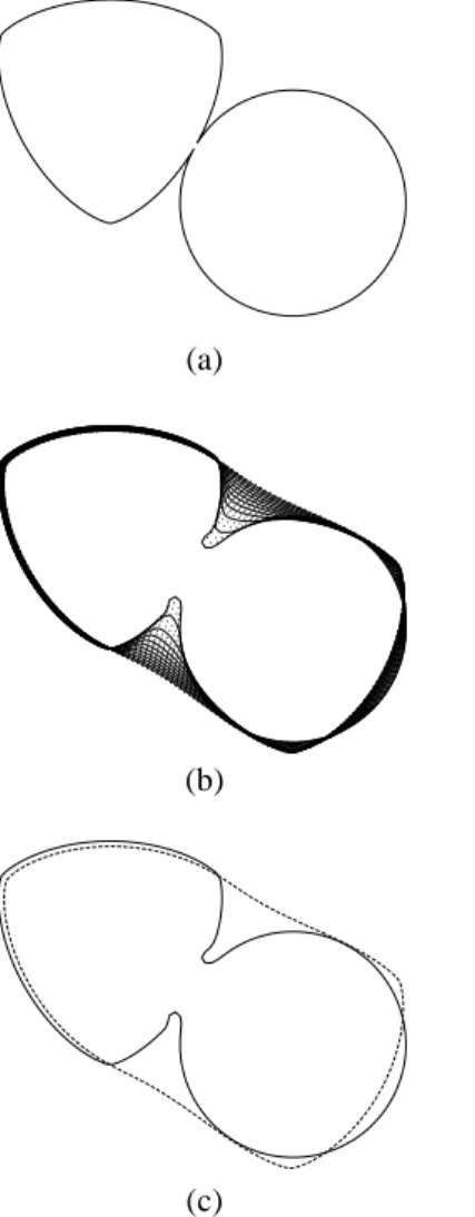
Breaking of a comparison principle. In Fig 6 we plot
the initial curve consisting of the union of the boundary of a Wulff shape∂Wσ(withσhaving degreem= 3) touched by
a circle with a sufficiently large circle with a radius r >1
(see section 7). As soon as it evolved by the anisoperimetric ratio gradient flow it intersects the stationary Wulff shape
∂Wσ. Numerically computed examples displayed in Fig 6
(a) and (c) correspond to those of the conceptual Fig 2.
IX. CONCLUSIONS
(a)
(b)
(c)
Fig. 6. Anisoperimetric ratio gradient flow breaking comparison principle.
REFERENCES
[1] S. B. Angenent, G. Sapiro and A. Tannenbaum, “On affine heat equation for non-convex curves,” J. Amer. Math. Soc., Vol. 11, pp. 601–634, 1998.
[2] J. Barrett, H. Garcke and R. N ¨urnberg, “Parametric approximation of isotropic and anisotropic elastic flow for closed and open curves”,
Numerische Mathematik, Vol. 120, pp. 489–542, 2012.
[3] M. Beneˇs, M. Kimura and S. Yazaki, “Second order numerical scheme for motion of polygonal curves with constant area speed”, Interfaces
and free boundaries, Vol. 11, pp. 515–536, 2009.
[4] A. Dinghas, “ ¨Uber einen geometrischen Satz von Wulff f¨ur die Gleichgewichtsform von Kristallen”, Zeitschrift f¨ur Kristallographie, Vol. 105, pp. 304–314, 1944.
[5] I. Fonseca and S. M ¨uller, “A uniqueness proof for the Wulff theorem”,
Proc. Roy. Soc. Edinburgh, Vol. 119A, pp. 125–136, 1991.
[6] N. Fusco, L. Esposito and C. Trombetti, “A quantitative version of the isoperimetric inequality: the anisotropic case”, Ann. Sc. Norm. Super.
Pisa, Vol. 5, pp. 619–651, 2005.
[7] M. E. Gage, “An isoperimetric inequality with applications to curve shortening”, Duke Math. J., Vol. 50(4), pp. 1225–1229, 1983. [8] M. E. Gage, “On area-preserving evolution equation for plane curves”,
Contemporary Mathematics, Vol. 51, pp. 51–62, 1986.
[9] M. E. Gage, “Evolving plane curves by curvature in relative ge-ometris”, Duke Math. J., Vol. 72(2), pp. 441–466, 1993.
[10] Y. Giga, “Anisotropic curvature effects in interface dynamics”, Sugaku
Expositions, Vol. 16, pp. 135–152, 2003.
[11] M. E. Gage and R. S. Hamilton, “The heat equation shrinking convex plane curves”, J. Differ. Geom., Vol. 23, pp. 69–96, 1986.
[12] M. Grayson, “The heat equation shrinks embedded plane curves to round points”, J. Differential Geom., Vol. 26, pp. 285–314, 1987. [13] T. Y. Hou, J. S. Lowengrub and M. J. Shelley, “Removing the stiffness
from interfacial flows with surface tension”, J. Comput. Phys., Vol. 114(2), 312–338, 1994.
[14] L. Jiang and S. Pan, “On a non-local curve evolution problem in the plane”, Comm. in Analysis and Geometry, Vol. 16(1), pp. 1–26, 2008. [15] Yu-Chu Lin and Dong-Ho Tsai, “Application of Andrews and Green-Osher inequalities to nonlocal flow of convex plane curves”, Journal
of Evolution Equations, Vol. 12, pp. 833–854, 2012.
[16] L. Ma and A. Zhu, “On a length preserving curve flow” Monatshefte
f¨ur Mathematik, Vol. 165(1), pp. 57–78, 2012.
[17] Y. Mao, S.L. Pan and Y. Wang, “An area-preserving flow for closed plane curves”, Int. J. Math., Vol. 24, No. 1350029, 2013.
[18] K. Mikula and D. ˇSevˇcoviˇc, “Evolution of plane curves driven by a nonlinear function of curvature and anisotropy”, SIAM Journal on
Applied Mathematics, Vol. 61(5), pp. 1473–1501, 2001.
[19] K. Mikula and D. ˇSevˇcoviˇc, “A direct method for solving an anisotropic mean curvature flow of plane curves with an external force”, Math. Methods Appl. Sci., Vol. 27(13), pp. 1545–1565, 2004. [20] K. Mikula and D. ˇSevˇcoviˇc, “Computational and qualitative aspects of evolution of curves driven by curvature and external force”, Comput.
and Vis. in Science, Vol. 6(4), 211–225, 2004.
[21] S.L. Pan and J.N. Yang, “On a non-local perimeter-preserving curve evolution problem for convex plane curves”, Manuscripta Math., Vol. 127, pp. 469–484, 2008.
[22] D. ˇSevˇcoviˇc and S. Yazaki, “Evolution of plane curves with a curvature adjusted tangential velocity”, Japan J. Indust. Appl. Math., Vol. 28(3), pp. 413–442, 2011.
[23] D. ˇSevˇcoviˇc and S. Yazaki, “Computational and qualitative aspects of motion of plane curves with a curvature adjusted tangential velocity”,
Math. Meth. in the Appl. Sciences, Vol. 35(15), pp. 1784–1798, 2012.
[24] G. Wulff, “Z ¨ur Frage der Geschwindigkeit des Wachstums und der Aufl ¨osung der Kristallfl¨aschen”, Z. Krist., Vol. 34, pp. 449–530, 1901. [25] Xiao-Li Chao, Xiao-Ran Ling and Xiao-Liu Wang, “On a planar area-preserving curvature flow”, Proc. Amer. Math. Soc., Vol. 141, pp. 1783–1789, 2013.