Application of Physics Model in prediction of the Hellas Euro election results

(1)

Research Article

Application of Physics Model in prediction of the Hellas Euro election results

M. P. Hanias1_{and L. Magafas}2_,*

1_{Technological and Educational Institute of Chalkis, GR 34400, Evia, Chalkis, Hellas} 2_{Department of Electrical Engineering, Kavala Institute of Technology, St. Loukas 65404 Kavala, Hellas.}

Received 5 June 2009; Revised 8 September 2009; Accepted 14 September 2009

Abstract

In this paper we use chaos theory to predict the Hellenic Euro election results in the form of time series for Hellenic political parties New Democracy (ND), Panhellenic Socialistic Movement (PASOK), Hellenic Communistic Party (KKE), Coalition of the Radical Left (SYRIZA) and (Popular Orthodox Rally) LAOS, using the properties of the reconstructed strange attrac-tor of the corresponding non linear system, creating a new scientific field called “DemoscopoPhysics”. For this purpose we found the optimal delay time, the correlation and embedding dimension with the method of Grassberger and Procassia. With the help of topological properties of the corresponding strange attractor we achieved up to a 60 time steps out of sample prediction of the public survey.

Keywords: DemoscopoPhysics, Chaos, Forecasting Model.

Journal of Engineering Science and Technology Review 2 (1) (2009) 104-111

Technology Review

www.jestr.org

1. Introduction

The present work proposes the use, for the first time, Physical models especially methods from non linear analysis, chaos theory, in order to predict and study the Euro election results of Hellas, defining the new scientific term called “DemoscopoPhysics” in the sense of application of physics models to social phenomena modelling. The term DemoscopoPhysics consists from two words Demoscopie and Physics. The first word is a Hellenic ancient word that means political survey. This work was inspired from the emerging field of economophysics while mainly consists of autonomous mathematical physics models that apply to the finan -cial markets. Now we try to use them particular aspects of the complex nonlinear dynamics of political survey in order to pre-dict the Hellenic Euro election results. The idea to apply chaotic analysis on samples concerning election results seems to be valid, since the election system is a complex system, like the system of economy and can be influenced by similar factors. Another point is that the political shocks and financial crisis are phenomena fre -quently happened, which are innate elements in chaotic systems so for their predictability it can be used the chaos theory. The idea is to analyze not the given dynamic system, which remains mostly unknown, but an image-system with the same topology that pre-serves the main characteristics of the genuine.

2. Public Survey Time Series

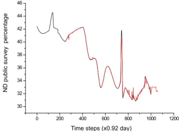
To construct the time series we have taken into account the as-sessment vote from public surveys in Hellas from 16-1-2007 to 23-04-2009 the estimation of the election behavior of the unclari-fied vote based on previous elections. The number of raw data is 36 for each political party, and each data is the average value of 4 polling companies with relative error 1%. In order to reconstruct of the equivalent phase space from experimental data the time-series that serves as experimental data should be constituted by sampled points of equal time-distances For this purpose we inter -polate with cubic spline so we take N=1000 points with a sample rate of 0.92day. The raw data and the interpolated public survey time series of the ND political party are shown at Fig.1, covering the period from 16-1-2007 to 23-04-2009. The sampling rate was Δt=0.92 days for all time series.

3. State Space Reconstruction

For a scalar time series, in our case the gallop poll time series the phase space can be reconstructed using the methods of delays. The basic idea in the method of delays is that the evolution of any sin-gle variable of a system is determined by the other variables with which it interacts. Information about the relevant variables is thus implicitly contained in the history of any single variable. On the basis of this an “equivalent” phase space can be reconstructed by assigning an element of the time series xi and its successive delays

as coordinates of a new vector time series . To construct a * E-mail address: [email protected]

(2)

vector , i=1 to N, in the m dimensional phase space we use the following equation [1-3]:

(1)

The Figs, 2, 3, 4, 5 shown the time series for PASOK, KKE, SYRIZA, LAOS, political parties respectively

represents a point to the m dimensional phase space in which the attractor is embedded each time, where τ is the time delay τ=iΔt. The element xi represents a value of the examined

scalar time series in time, corresponding to the i-th component of the time series. The dimension m of the re-constructed phase space is considered as the sufficient di-mension for recovering the object without distorting any of its topological properties, thus it may be different from the true dimension of the space where this object lies. Use of this method reduces phase space reconstruction to the prob-lem of proper determining suitable values of m and τ. The next step is to find time delay (τ) and embedding dimension (m) without using any other information apart from the his-torical values of the indexes. This is why the methodology is labelled as a stochastic one. We can calculate the time delay by using the aver

-age mutual [4-6] information presented in equation (2):

(2)

In this equation, P(xi) is the probability of value xiand P(xi,

xi+τ) denotes joint probability. I(τ) shows the information (in bits)

Figure 1. Interpolated time series for ND public survey for period 16-1-2007

to 23-04-2009, (black line) and raw data (red dots).

Figure 2. Interpolated time series for PASOK public survey for period from

16-1-2007 to 23-04-2009, (black line) and raw data (red dots).

Figure 3. Interpolated time series of KKE public survey for period from

Figure 4. Interpolated time series of SYRIZA public survey for period from

Figure 5. Interpolated time series of LAOS public survey for period from

(3)

being extracted from the value in time xi about the value in time

xi+τ. The time delay is calculated by using the first minimum of the

mutual information [2]. Mutual information against the time de -lays for the time series of ND, PASOK, KKE, SYRIZA and LAOS political parties are presented in Figs. 6, 7, 8, 9, 10, respectively.

From Fig .6 we find that the nadir of Mutual Information for ND time series ia at τ=37.

From Fig 7 we find that the nadir of Mutual Information for PASOK time series is at τ=20.

From Fig. 8 we find that the nadir of Mutual Information for KKE time series is at τ=28.

From Fig 9 we find that the nadir of Mutual Information for SYN time series is at τ=40.

From Fig .10 we find that the nadir of Mutual Information for LAOS time series is at τ=23.

With the above method we found the τ as the time neces-sary to cancel the correlation between two time series values to be 37, 20, 28, 40, 23 time steps for ND, PASOK, KKE, SYRIZA and LAOS, respectively. One method to determine the presence of chaos is to calculate the fractal dimension, which will be non integer for chaotic systems. Even though there exists a number of definitions for the dimension of a fractal object (Box counting di -mension, Information Di-mension, etc.), the correlation dimension was found to be the most efficient for practical applications [7, 8]. Firstly, we calculate the correlation integral for the time series for lim r0 and N∞ by using equation (3) [2]:

(3)

Figure 6. Mutual Information (I) vs time delay (τ) for ND political party.

Figure 7. Mutual Information (I) vs time delay (τ) for PASOK political party.

0 20 40 60 80 100

1.0 1.5 2.0 2.5 3.0 3.5

I(

τ)

τ

Figure 8. Mutual Information (I) vs time delay (τ) for KKE political party.

Figure 9. Mutual Information (I) vs time delay (τ) for SYRIZA political

party.

Figure 10. Mutual Information (I) vs time delay (τ) for LAOS political

(4)

In this equation, the summation counts the number of pairs for which the distance, (Euclidean norm), i s less than r, in an m dimensional Euclidean space. Η is the Heavi -side step function, with H(u) = 1 for u > 0, and H(u) = 0 for u ≤ 0, where , Ν denotes the number of points and expressed in equation (4):

(4)

Where r is the radius of the sphere centered on Xi or Xj. If the

time series is characterized by an attractor, then for positive values of r, the correlation function is related to the radius with a power law C(r)~αrv, where α is a constant and ν is the correlation dimension or

the slope of the log2Cm(r) versus log2 r plot. Since the data set will

be continuous, r cannot get to close to zero. To handle this situation, from the log2C(r) versus log2r plots we select the apparently linear

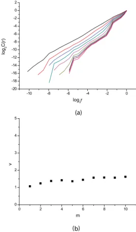
portion of the graph. The slope of this portion will approximate ν. Practically, one computes the correlation integral for increasing em-bedding dimension m and calculates the related ν(m) in the scaling region. Using the appropriate delay times for each political party i.e, 37, 20, 28, 40, 23 time steps for ND, PASOK, KKE, SYRIZA and LAOS, respectively, we reconstruct the phase space for ND. The correlation integral C(r), by definition is the limit of correlation sum of equation (3) for embedding dimensions m=1..10. is shown in Fig 11(a), while in Fig.11 (b), the corresponding average slopes

v are given as a function of the embedding dimension m, indicating that for high values of m, v tends to saturate at the non integer value of v=1.6. The embedding dimension m is found to be m ≥ 2[v]+1=3

where [v] is the integer part of v [2].

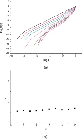
Applying the same procedure for PASOK political party we show in Fig 12 (a) the relation between log2C(r) and log2r for

dif-ferent embedding dimensions m, while in Fig.12 (b), the corre -sponding average slopes v are given as a function of the embed-ding dimension m indicating that for high values of m, v tends to saturate at the non integer value of v=1.53. The embedding dimen -sion m is found to be m ≥ 2[v]+1=3 [2].

For KKE we show in Fig 13 (a) the relation between log2C(r)

and log2r for different embedding dimensions m, while in Fig.13

(b), the corresponding average slopes v are given as a function of the embedding dimension m indicating that for high values of m, v tends to saturate at the non integer value of v=1.28. The embed -ding dimension m is found to be m ≥ 2[v]+1=3 [2].

2

)

1 (

2 +

−

=

m

N

_pairs

Figure 11. (a) Relation between log2C(r) and log2r for different embedding

dimensions m. (b) Correlation dimension v vs. embedding dimen

-sion m for ND.

(5)

For SYRIZA we show in Fig 14 (a) the relation between log2

C(r) and log2r for different embedding dimensions m, while in

Fig.14 (b), the corresponding average slopes v are given as a func-tion of the embedding dimension m indicating that for high values of m, v tends to saturate at the non integer value of v=1.29. The

embedding dimension m is found to be m ≥ 2[v]+1=3 [2].

For LAOS we show in Fig 15 (a) the relation between log2

C(r) and log2r for different embedding dimensions m while in

Fig.15 (b), the corresponding average slopes v are given as a func-tion of the embedding dimension m indicating that for high values

of m, v tends to saturate at the non integer value of v=1.23. The

embedding dimension m is found to be m ≥ 2[v]+1=3 [2].

Table 1 shows the results from previous analysis

We can see from Table 1 that the smaller political parts have smaller correlation dimension. We can interpret it that the smaller are more robust to keep there voters but on the other hand they cannot adapt changes as the larger parties do.

4. Time Series Prediction

The next step is to predict evolution of the percentages of votes for each political party, by computing weighted average of evolu-tion of close neighbors of the predicted state in the reconstructed

-sion m for KKE.

-sion m for SYRIZA.

-sion m for LAOS.

Political parties Correlation dimension ν

ND 1.60

PASOK 1.53

KKE 1.28

SYRIZA 1.29

LAOS 1.23

(6)

phase space [9-12]. The reconstructed m-dimensional signal pro-jected into the state space can exhibit a range of trajectories, some of which have structures or patterns that can be used for system prediction and modeling. Essentially, in order to predict k steps into the future from the last m-dimensional vector point we have to find all the nearest neighbors in the ε-neighborhood of this point. To be more specific, let be the set of points within ε of (i.e. the ε-ball). Thus any point in is closer to the than ε. All these points come from the previous trajectories of the system and hence we can follow their evolution k-steps into the future . The final prediction for the point is obtained by averaging over all jections k-steps into the future. The algorithm can be written as

(5)

w h e r e denotes the number of nearest neigh-bors in the neighborhood of the point [2. As an example we suppose that we want tο predict k=2 steps ahead. The basic principle of the prediction model is visualized in Fig 16. The blue dot represents the last known sample, from which we want to predict one and two steps into the future. The blue circles rep -resent ε-neighborhoods in which three nearest neighbors were found.

The next step in the algorithm is to check that the projections, one and two steps into the past, of the points in are also nearest neighbors of the two previous readings a n d , respectively. This criterion excludes unrelated trajec -tories that enter and leave the ε-neighborhood of but do not “track back” to ε-neighborhoods of and

thus making them un-suitable for prediction. Assuming that any nearest neighbors have been found and checked using the criterion detailed previously, we project their trajectories into the future and average them to get results for and . We used the values of τ and m from our previous analysis so the appropri -ate time delays τ as before. We use as embedding dimension the 2*m = 6 [13] for all predictions. Actual and predicted time series

for k=60 time steps ahead are presented at Figs 17, 18, 19, 20, 21, for ND, PASOK, KKE, SYRIZA, LAOS, respectively.

,

, neighbors’

pro-,

,

Figure 16. Basic prediction principle of the simple deterministic model.

} { m N x } { m N x } { 1 m N x − } { 2 m N x − } { 1 m N x + } { 2 m N x + , ,

Figure 17. Actual (black line) and predicted (red line) time series for n=60

time steps ahead or ND political party. The parameters are m=6, τ=37, number of near neighborhoods, nn=35.

time steps ahead for PASOK political party. The parameters are m=6, τ=20, number of near neighborhoods, nn=8.

(7)

At table 2 we present our out of sample estimation about polit-ical survey estimation for two characteristic dates The first 25/5/09 corresponds to 33 time steps ahead while the second 7/6/2009 (Eu -ropean election date) corresponds to 50 time steps ahead.

At this point we mark that until 23/4/2009 we had not data for Ecological Party. This political party, generally speaking, is in cognation with Coalition of the Radical Left (SYRIZA) so its presence can affect SYRIZA’s percentage.

5. Conclusions

In this paper, we use a chaotic analysis to predict Hellenic Euro election results. After estimating the dependence of correlation di -mension on embedding di-mension, we point out that the system is a deterministic chaotic. A separate attractor for each political party, embedded in 3-D space, is derived from the analysis. How -ever the election system is obviously a complex multi-variable system with strong inter-relation between variables. In this sense, we have model each separate time series and never the whole elec-tion system, whose attractor is obviously much more complex. From absolute values of correlation dimension we see that the smaller political parts have smaller correlation dimension. We can interpret it that the smaller are more robust to keep there vot-ers but on the other hand they cannot adapt changes as the larger parties do. From reconstruction of the systems’ strange attractors, we achieve a 60 time steps out of sample prediction. As the time horizon increases the prediction becomes weak. This depends on strange attractor’s structure and the number of raw data. As this number increases the influence of cubic spline is reduced and the results will be more precise. As seen before the in sample predic -tion works well so we believe that the out of sample predic-tion gives satisfactory results. Of course if we could include data for Ecological Party our prediction will be more accurate. Using tools and principles from Physics as the number of freedoms and the topological properties of strange attractor we try modeling an open humanitarian systems as a National and Euro election system are. Of course this is a preliminary effort. To establish a new term as DemoscopoPhysics we need more data for testing and more tools from Physics to apply as entropy and criticality and phase transi-tion are. The future researches may concentrate on the alternative models (i.e. parametric and nonparametric ones) for prediction. In addi-tion, to reflect the time-scaling effects and wavelet theory which can be combined with the chaos theory.

time steps ahead for SYRIZA political party. The parameters are m=6, τ=40, number of near neighborhoods, nn=20.

time steps ahead for LAOS political party. The parameters are m=6, τ=23, number of near neighborhoods, nn=3.

Political parties

25/5/2009 political survey

estimation %

7/6/2009 political survey

estimation %

ND 32.98420 32.33710

PASOK 39.21590 37.19480

KKE 8.72589 8.52282

SYRIZA 7.54657 7.48410

LAOS 6.64646 6.81252

(8)

1. Takens F.: Detecting strange attractors in turbulence, Lecture notes in Mathematics, vol. 898, Springer, New York (1981).

2. Kantz H. and T. Schreiber: Nonlinear Time Series Analysis, Cambridge University Press, Cambridge, (1997).

3. Kennel M.B., Brown R., Abarbanel H.D.I.: “Determining embedding

dimension for phase-space reconstruction using a geometrical

construc-tion”, Phys. Rev. A, 45, 3403, (1992).

4. Abarbanel H.D.I.: Analysis of observed chaotic data, Springer, New York, (1996).

5. Fraser A.M., Swinney H.L.: Independent coordinates for strange attractors from mutual information, Phys. Rev. A, 33, 1134, (1986).

6. Kugiumtzis D., Lillekjendlie B., Christophersen N.: Chaotic time series, Part I, Modeling Identification and Control 15, 205, (1994)

7. Grassberger, P. and I. Procaccia: Phys. Rev Lett., 50, 346-34, 1983. 8. Miksovsky J., Raidl A.: On some nonlinear methods of meteorological

time series analysis, proceedings of WDS 2001 Conference (2007).

9. Stam C.J., Pijn J.P.N., Pritchard W.S.: Reliable detection of nonlinearity in experimental time series with strong periodic component, Physica D, vol. 112, 361, (1998)

10. Hanias M.P., P.G. Curtis, J.E. Thallasinos: “Non-Linear Dynamics and Chaos: The case of the Price Indicator at the Athens Stock Exchange”, International Research Journal of Finance and Economics, Issue 11, pp. 154-163 (2007).

11. Hanias, P. Curtis and J. Thalassinos: “Prediction with Neural Networks: The Athens Stock Exchange Price Indicator”, European Journal of Eco

-nomics, Finance And Administrative Sciences - Issue 9 (2007). 12. Hanias M.P. and D.A. Karras: “Efficient Non Linear Time Series Predic

-tion Using Non Linear Signal Analysis and Neural Networks in Chaotic

Diode Resonator Circuits”, Springer Berlin / Heidelberg Lecture Notes in Computer Science, Advances in Data Mining. Theoretical Aspects and ApplicationsVolume 4597, pp 329-338 ( 2007).

13. Sprott J.C.: Chaos and Time series Analysis, Oxford University Press, (2003).