www.ann-geophys.net/26/813/2008/ © European Geosciences Union 2008
Annales
Geophysicae
Universal and local time components in Schumann resonance
intensity
A. P. Nickolaenko1and M. Hayakawa2
1Usikov Institute for Radio-Physics and Electronics, National Academy of Sciences of the Ukraine, Kharkov 61085, Ukraine 2The University of Electro-Communications, Department of Electronic Engineering, Chofu-shi, Tokyo, 182-8585, Japan
Received: 4 April 2007 – Revised: 28 February 2008 – Accepted: 13 March 2008 – Published: 13 May 2008
Abstract. We extend the technique suggested by Sent-man and Fraser (1991) and discussed by Pechony and Price (2006), the technique for separating the local and universal time variations in the Schumann resonance in-tensity. Initially, we simulate the resonance oscilla-tions in a uniform Earth-ionosphere cavity with the dis-tribution of lightning strokes based on the OTD satellite data. Different field components were used in the Day-side source model for the Moshiri (Japan, geographic coor-dinates: 44.365◦N, 142.24◦E) and Lehta (Karelia, Russia, 64.427◦N, 33.974◦E) observatories. We use the extended Fourier series for obtaining the modulating functions. Sim-ulations show that the algorithm evaluates the impact of the source proximity in the resonance intensity. Our major goal was in estimating the universal alteration factors, which re-flect changes in the global thunderstorm activity. It was achieved by compensating the local factors present in the ini-tial data. The technique is introduced with the model Schu-mann resonance data and afterwards we use the long-term experimental records at the above sites for obtaining the di-urnal/monthly variations of the global thunderstorms. Keywords. Meteorology and atmospheric dynamics (Atmo-spheric electricity; Lightning) – Radio science (Remote sens-ing)
1 Introduction
Global electromagnetic (Schumann) resonance occurs in the thin dielectric shell separating the conducting ground and the ionosphere plasma. It is observed as peaks in the intensity of natural radio noise at frequencies around 8, 14, 20 Hz, etc. The energy is supplied by electromagnetic radiation from the lightning strokes distributed worldwide. Owing to low losses Correspondence to:M. Hayakawa
a radio wave can circle the globe several times, and the in-tensity recorded reflects the level of global thunderstorm ac-tivity. Observations at a field site are characterized by two factors: one depends on the universal time (the global thun-derstorm intensity) and the other is the function of the local time (local ionosphere height, position of thunderstorms rela-tive the observatory, etc.). The first depends on the Universal Time (tU), while the second is a function of the Local Time
(tL).
When monitoring the global thunderstorm activity by us-ing Schumann resonance (SR), one has to reduce the role of the local factors and preserve the universal modulations. For this purpose, the cumulative resonance intensity was suggested and used by Polk (1969), which is the resonance field intensity integrated over a few SR modes. The advan-tage of cumulative intensity is conditioned by smoothing the distance dependence pertinent to different resonant modes. Model computations showed that an effect of diurnal motion of global thunderstorms decreases from∼10 dB variation in the individual modes toward∼3 dB in the cumulative inten-sity (Nickolaenko, 1997). Thus, the role of source proximity is reduced by the cumulative intensity, but it is not removed completely. In the present paper, we modify a technique that separates the local and universal factors and estimate the level of global thunderstorms by using the cumulative SR in-tensity recoded at a pair of longitudinally separated observa-tories.
A first comparison of SR intensities recorded at two widely separated observatories was made by Polk and Fitchen (1962), in which measurements were made at Bran-nenburg (Germany) and Kingston (R.I., USA). Their experi-ment indicated that diurnal variations at two points look more similar when plotted against the local time rather than in the universal time.
experimental cumulative intensity and singled out the peri-odic local factor. The sites were positioned at California and Australia. The local changes derived were attributed to alter-ations in the local ionosphere height above each site.
The further step was made by Pechony and Price (2006), who computed the intensity of the global resonance in the model of a uniform Earth-ionosphere cavity and demon-strated that local modulations still remain in the model data. They used the time varying thunderstorm distributions in model that follow from the records of Optical Transient De-tector (OTD) satellite. Thus the above work showed that the local time variations arise from a diurnal motion of thunder-storm activity around the globe, i.e. from the source proxim-ity. Magnitude of model variations was close to that observed experimentally by Sentman and Fraser (1991).
The goal of the present publication is two-fold. First, we adopt a similar technique to the case of a slightly different source distribution in comparison with Pechony and Price (2006). Such a numerical experiment allows us to test the ro-bustness of our processing. Second, we extend the number of terms in the Fourier expansion from 1 to 5 and therefore ac-quire more sophisticated temporal variations. The processing technique is also developed aiming on the direct extraction of universal or local time factors.
Initially, we describe the procedure and process a model signal to demonstrate applicability of the technique. The model intensity variations were computed in the uniform Earth-ionosphere cavity with the thunderstorm distribu-tion based on the global OTD maps of lightning flashes (Hayakawa et al., 2005; Nickolaenko et al., 2006; Pechony et al., 2006). We compare the “postulated” source intensity with the universal factor “deduced” from the SR and thus evaluate the accuracy. The algorithm is finally applied to the long-term experimental records of SR at the same two points and the estimates are found for diurnal/monthly variations of the global thunderstorm activity for the period one year long.
2 Formal treatment
Similarly to Sentman and Fraser (1991), we accept that (i) Intensity of SRP (tU,λ) recorded in the universal time
tU and at the east longitudeλis a product of the universal
functionU(tU)and the local modulating functionL(tL):
P (tU)=U (tU)·L (tL) (1)
Additionally, we present the same data against the local time tL, which is used later for the direct extracting of the
univer-sal component instead of the local time variation:
Q (tL)=U (tU)·L (tL) (2)
HereP (tU)denotes the SR intensity recorded in the
univer-sal timetU,Q(tL)is the same intensity as the function of the
local time of the observatorytLthat occupies the east
longi-tudeλ.U(tU)andL(tL)are the universal and local factors
to be found. Equations (1) and (2) are used for an arbitrary observatory.
(ii) The following relation is valid (Sentman and Fraser, 1991):
tL=tU+λ, (3)
with all quantities measured in radians and ranging from 0 to 2π.
(iii) Functions P andQ at an observatory are the same functions of time. The only distinction is in the shift along the abscissa in correspondence with Eq. (3). Of course, devi-ations might occur in the data calibrationP1,Q1andP2and
Q2at different observatories. These might cause different
amplitude scaling (similar distinctions might arise from the different latitudes of the sites).
(iv) Since functionsU(tU)andL(tL)have a period of 2π,
we expand them into the following Fourier series:
L1(tU)=1+
∞ X
k=1
Akexp [ik (tU+λ1)]
L2(tU)=1+
∞ X
k=1
Akexp [ik (tU+λ2)] (4)
Similarly, we develop relations for the universal modulating functions. The procedure is also the Fourier expansion and only initial SR intensities must be presented versus the local time of observatories instead of the UT. Formally, we obtain the following series for the normalized universal modulating factors:
u1(tL)=1+
∞ X
k=1
Bkexp [ik (tL−λ1)]
u2(tL)=1+
∞ X
k=1
Bkexp [ik (tL−λ2)] (5)
Here,L1andL2is the local modulations at each site. The
functions are found by using Eq. (1). The normalized univer-sal modulating factors at the sites are denoted asu1andu2,
they depend on the local time of observatories, and will be found by usingQ1(tL)andQ2(tL)records.
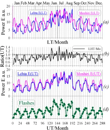
The upper frame (a) in Fig. 1 depicts theQ(tL)–
func-tions, the third frame (c) presents theP (tU)– variations.
Co-ordinates of two observatories were used. One is Lehta (ge-ographic coordinates: 64.427◦N and 33.974◦E), whose data are shown by blue curves. The second is Moshiri (44.365◦N and 142.24◦), with the relevant graphs in the magenta lines. As one may observe, the plots vary similarly against the UT, i.e. in Fig. 1c. Mutual departures of two curves in the UT are demonstrated by Fig. 1b in form of the ratioP1(tU)/P2(tU).
We return to the data of Fig. 1 later. Here, we must note a higher similarity of the patterns in the UT, which validates the assumption (iii).
Expansion (4) corresponds to the formula used by Sent-man and Fraser (1991). The distinction is that they have used a single harmonic only. We use the five terms expan-sionsk∈[1; 5]. Similarly to Sentman and Fraser (1991), we use the UT recordsP1(tU)andP2(tU)for deriving the local
time factors (Eq. 4). The expansion coefficients are found from the following equation:
Ak=
1 2π
exp(ikλ1)−exp(ikλ2) 2π
Z
0
ln P
1(tU)
P2(tU)
exp(−iktU) dtU (6)
The local factorsL1(tU)andL2(tU)are reconstructed with
the coefficientsAksubstituted into Eq. (4).
Our goal is obtaining universal variations U1(tU) and
U2(tU)representing the current intensity of the global
thun-derstorms. To find the universal factors directly, we apply the SR records (Eq. 2) performed in the local timesQ1(tL)
andQ2(tL). The expansion coefficients for the “normalized”
universal factors are:
Bk =
1 2π
exp(−ikλ1)−exp(−ikλ2) 2π
Z
0
ln Q
1(tL)
Q2(tL)
exp(−iktL) dtL (7)
After finding quantities Bk, we construct functions u1(tL)
andu2(tL)by using Eq. (5), and afterwards we compute the
genuine functionsU1(tL),U2(tL):
Um(tL)=um(tL)·Qm(tL) m = 1, 2 (8)
with the average intensity at a site:
Qm(tL)=
1 2π
2π
Z
0
Qm(tL) dtL. (9)
Finally, the local timestLof observatories are translated into
the universal time, and we obtain the functionsU1(tU)and
U2(tU). The last procedure provides two “independent”
esti-mates for the global thunderstorm activity. Their consistency reflects the robustness of the procedure.
Fig. 1.A set of twelve model diurnal patterns, each corresponding to a month. Frame(a)depicts theQ(tL)data and frame(c)is the
P (tU)variations. Intensities are measured in arbitrary units. Data
for Lehta are shown by blue line and for Moshiri – by magenta line. Plot(b)depicts the intensity ratioPLEHTA/PMOSHIRI, and the lower green dotted curve presents the source intensity.
By comparing Eqs. (6) and (7), we find only minor distinc-tions. The sign has changed of the “longitudinal” argument in the denominator; the integration is performed overtU in
Eq. (6) and overtLin Eq. (7). Since this is the “umbral”
ar-gument, the result does not depend on the type of particular variable. Hence, expansions of the local and the normalized universal functions are obtained by essentially the same pro-cedure. The key distinction is that initial data are related to the LT when we obtain the universal factor, and to the UT when we obtain the local modulation factor.
We use below the SR records 24 h long, and an extension to a wider interval is rather straightforward. The Fourier co-efficients might be computed directly or by using the stan-dard FFT procedure.
To conclude the formal description, we mention the sim-plest possible signal processing: the geometrical averaging. Let us assume that two observatories have the longitudinal separation of 180◦or (λ1–λ2)=±π. The basic terms in the
lo-cal modulating functionsL1(tL)andL2(tL)having the 24 h
universal terms:
S=ln [P (tU, λ)]+ln [P (tU, λ+π )]
≈U (tU)[1+ReA1(tU)]+U (tU)[1−ReA1(tU)]
=2U (tU) (10)
Equation (10) indicates that geometrical averaging of inten-sities
GA=pP (tU, λ1)·P (tU, λ2) (11)
represents the “rectified” universal variations. Physical ex-planation of this effect is simple: when storms come closer to one observatory, they simultaneously retreat from the other, so that the product of individual SR intensities tends to be independent of the source distance. When (λ1–λ2)=±π, we
exactly haveGA=U (tU). When observatories are separated
in longitude by a smaller value (or their latitudes are differ-ent), the compensation is incomplete of the local modula-tions.
The idea of geometric averaging is easily extended to the case of many sites. For instance, when we have three ob-servatories (separated by 2π/3 in longitude), the global thun-derstorm intensity is evaluated byU (tU)=√3P1·P2·P3, etc.
Simple geometrical averaging of the UT data provides an es-timate for the intensity of the global thunderstorms. Vice versa, the procedure applied to intensities recorded in the lo-cal time provides an estimate for the lolo-cal modulating func-tion. We show with the model data that geometrical averag-ing is as efficient as a more complicated Fourier expansion algorithm.
3 Modeling of the SR data
After formulating the main points of data processing, we turn to computing the SR spectra and obtaining variations of cu-mulative intensity at two points of longitudesλ1andλ2. In
particular, we use observatories separated both in longitudes and latitudes: Lehta (Karelia) and Moshiri (Hokkaido). We use the uniform model of Earth – ionosphere cavity. Fre-quency dependence of the propagation constant is approx-imated by the following linear function (Nickolaenko and Hayakawa, 2002):
ν (f )= f−2 6 −i
f
70 (12)
Let us test the above modifications of the Sentman and Fraser (1991) approach. In addition we compare our data with con-clusions by Pechony and Price (2006) based on a different source model.
One might use, say, the single point source model (Yatse-vich et al., 2006) for the purpose, or the model of three global thunderstorm centers (Nickolaenko et al., 1998) and syn-thesize the necessary “experimental” data set. Clearly, the
model data should be realistic, therefore, we use the follow-ing approach. The global thunderstorm distribution was ob-served from space by the Optical Transient Detector (OTD) (Christian et al., 2003), and we use the low resolution full climatology dataset with the step of 2.5 by 2.5 degrees. To introduce the daily motion of thunderstorms, we apply the Dayside (DS) model (Nickolaenko et al., 2006; Pechony et al., 2006). This model is the mask covering the dayside of the globe for the specific date and the time (UT). The mask is ap-plied to the OTD map relevant to a particular month, and the lightning flashes are “active” within the dayside, while those at the night side do not occur. The mask circles the globe during the day, thus the daily motion of thunderstorm activ-ity appears in the averaged optical observations from space. To improve correspondence to the reality, we “rotate” the DS mask toward the evening terminator so that its center (the potential peak of activity) is placed at 17:00 LT.
Strokes within individual cells of the OTD map are inde-pendent and form a Poisson succession of electromagnetic pulses, therefore, their intensities are summed. The contri-bution from a particular cell is directly proportional to the number of flashes here. Such a model allows for comput-ing the intensity of any field component or any second-order mixed statistical moments of the fields (Nickolaenko et al., 2006; Pechony et al., 2006). We computed the power spectra ofEZfield component at a site for the given hour UT and for
the 15th day of each month. Afterwards, we integrated the field intensities in the frequency band from 4 to 26 Hz and obtained the functionsP1(tU),P2(tU)andQ1(tL),Q2(tL)
plotted in Fig. 1.
Every frame in Fig. 1 combines 12 diurnal patterns shown against the local (Fig. 1a) and universal time (Fig. 1c). The 24 h diurnal alterations follow each other in correspondence with the month starting from January.
Model diurnal patterns at two distant observatories have much in common. Field intensity noticeably increases dur-ing the summer. As we already noted, alterations become es-pecially similar when plotted against the universal time (see Fig. 1c), which confirms the general idea that the cumula-tive SR intensity closely represents the global thunderstorm activity. The lower plot (Fig. 1d) is a reference, and it de-picts the cumulative number of lightning flashes recorded by the OTD satellite. The model source intensity is pro-portional to this quantity. In an ideal case, when the spatial modal structure of resonance oscillations is completely com-pensated, the SR records must coincide with the reference curve. Our computations indicate that reciprocity undoubt-edly exists, but curves do not coincide completely.
4 Extracting the local factors
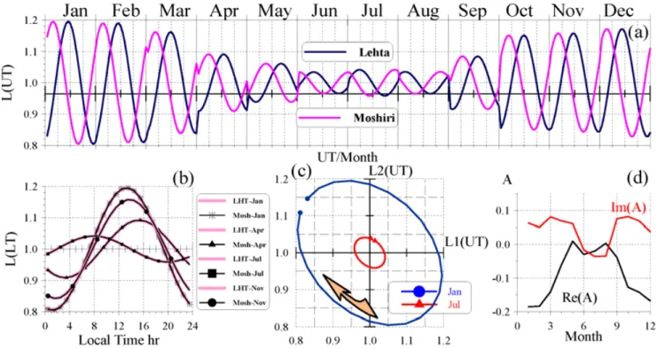
Fig. 2.Local modulation functions for model Schumann resonance records at Lehta and Moshiri extracted by the Sentman and Fraser (1991) algorithm. A single term in the Fourier series.
initial data are the functions of the universal time, and we exploit only theA1Fourier coefficient.
Figure 2a surveys monthly/diurnal alterations of the mod-ulating functions L1 (Lehta) and L2 (Moshiri) versus UT.
Again, twelve diurnal patterns are shown, each correspond-ing to different month. We observe that local modulations increase in winter and decrease in summer, and the position of peak depends on the season. Figure 2b compares the same variations plotted in the local time. The wide pink lines here depict the Lehta data, while results for Moshiri are plotted by narrow black marked lines. Characteristic months were chosen: January, April, July, and November. We must recall here that Sentman and Fraser (1991) have noted an outstand-ing similarity of these curves and attributed them to varia-tions of the local ionosphere height. Such an interpretation looks reasonable if we accept that cumulative SR intensity is completely independent of the source – observer geometry. Unfortunately, this is not so because the ionosphere height is an invariant in our model of the uniform cavity and only source motion might cause variations in our data. Thus our computations support the conclusion by Pechony and Price (2006) based on different cavity and the source model. Phys-ically, Fig. 2 shows that cumulative resonance intensity does not completely remove the modal structure, and the effect of source proximity is still present in the data.
Figure 2c shows the impact of seasonal redistribution of global thunderstorms on the peak positioning in the L-functions. We use January and July data here depicted as
Lissajous plots (time UT∈[1; 24] is the parameter). The ar-row shows the clockwise temporal motion of the represent-ing point; the startrepresent-ing and the final points are marked. One may see that only two parameters of ellipses vary with sea-son: the size and position of initial/ending points. Ellipticity and orientation of the curve remain stable regardless the sea-sonal drift of thunderstorms. The ellipticity depends on the longitude separation of the sites, and the Lissajous plots are the wide ellipses forλ1–λ2=110◦. For the 90◦separation the
plot would become a circle, and it is the straight line for 180 degrees. Such a behavior of our model data agrees with the experimental results published by Polk and Fitchen (1962). Figure 2d explains why the initial phase of sinusoidal pat-tern varies with the month: alterations are caused by changes in the imaginary and real parts of the complex A1
ampli-tude. The black line depicts Re{A1}, and the red line shows
Im{A1}.
We conclude that our model data support the conclusion made by Pechony and Price (2006): the local time variations remain in the cumulative SR intensity, and these alterations are connected with the diurnal/seasonal motion of thunder-storms around the globe.
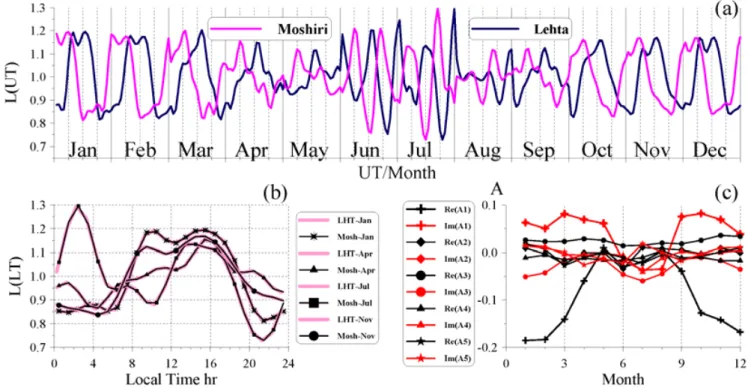
After repeating the processing suggested by Sentman and Fraser (1991), we extend the number of Fourier coefficients in an attempt to obtain the detailed variations. We use five harmonics in Eq. (6) and substitute these into the series (4). Relevant local modulating functionsL1andL2are shown in
Fig. 3.Local modulation functions for Lehta and Moshiri obtained with a series of five terms in the Fourier series.
modulations against UT. One can observe that additional terms substantially modify the patterns. Now, the smallest modulation occurs in the intermediate seasons, which is in accord with observations of the first SR frequency: the thun-derstorms “spread” over the globe during the intermediate seasons (Nickolaenko and Rabinowicz, 1995; Nickolaenko et al., 1998).
Figure 3b shows the modulation factorsL1andL2against
the local time. We plot the Lehta data by wide magenta lines, and those for Moshiri by the narrow black marked lines. The same four characteristic months were used for the seasons. One may observe that plots became complicated, however, their similarity was preserved. It is interesting to note that Fig. 3b indicates the smallest source – observer distance around 16:00 LT, which agrees with the general de-scription of thunderstorm development. The morning peak around 10:00 h probably reflects the thunderstorm activity in the South-East Asia. The nighttime summer peak should be attributed to thunderstorm activity at the West coast of the North America. Since we perform a “controlled” numeri-cal experiment, we can readily check the above interpreta-tions with the OTD maps and with the relevant variainterpreta-tions in the flash number (Nickolaenko et al., 2006; Pechony et al., 2006). Figure 3c illustrates the behavior of the complexAn
coefficients for five Fourier termsn∈[1; 5].
We can derive the universal functionsU1andU2now by
dividing initial intensitiesP1andP2by modulating functions
L1andL2. This is an obvious way for obtaining the universal
modulations as a proxy of the global thunderstorm activity.
TheU1andU2functions obtained will be regarded as
“re-covered”, which are depicted in Fig. 5a. FunctionsU alter similarly in general, and deviations appear in summer. How-ever, correspondence of theU1 andU2 patterns in Fig. 5a
is less pronounced than that of the local modulating func-tionsL. Plots (c) in Fig. 5 show that geometric averages are also close to each other and to the recovered universal mod-ulations. Data are also similar to the “input” source intensity shown by the lowest line in Fig. 5d. We must note that simple geometrical averaging procedure provides results as good as more complicated procedures of evaluating theL-functions first and deriving theU-function afterwards.
5 Extracting the model universal factors
We described an alternative variant of the data processing, which is based on Eqs. (5) and (7). It allows us to di-rectly reconstruct variations of the universal factors u1(tL)
andu2(tL). The results are presented in Fig. 4a in the
man-ner similar to that of Fig. 3a. Figure 4a surveys the diur-nal/monthly alterations of the “normalized thunderstorm ac-tivity” against the local times of Lehta (dark blue line) and Moshiri (magenta curve). As we see, the estimated source activity varies substantially up to ten times, and the peak-to-peak alterations decrease almost to two-fold level during the summer season.
Fig. 4. Universal modulation functions: the normalized –u(UT) and the “absolute” –U(UT) obtained from the Lehta and Moshiri model data with a series of five terms.
translated from the LT to UT with the help of Eq. (3). Fig-ure 4b compares the daily patterns u1(tU) andu2(tU) for
twelve months of a year. Wide blue line presents the Lehta data, and data for Moshiri are depicted by magenta line. Plots in Fig. 4b practically coincide. After multiplying the normal-ized patterns by the daily average intensities at relevant sites (9), we obtain the “absolute” curvesU1(tU)andU2(tU)
pre-sented in Fig. 4c. The “scaling factor” separates individual patterns. The coincidence is retained for some months. De-viations are conditioned by an inequality of the median dis-tance from the sources to the observatories: we use the sites separated not only by the longitude, but also along the lati-tude. In experimental studies, similar deviations might also arise from departures in the data calibration.
6 Comparison of universal patterns recovered
We compare in Fig. 5 all kinds of variations obtained for the universal time factors U. The upper plots show the “recovered” data when the local modulations were found first, and the functionsU1(UT) andU2(UT) were derived by
compensating the local modulationsL1(UT) andL2(UT) in
the recordsP1(tU)andP2(tU). The dark blue curve
corre-sponds to the Lehta data and the magenta line depicts those of Moshiri. The green line is the reference curve: the postulated
Fig. 5. Survey of universal modulations. Curves(a)depict the re-sults after compensating the local factorsL. Curves(b)show the results of direct evaluation ofU(UT) by using the Q1/Q2ratio. Curve(c)is the geometric averageGA(tU), and curve(d)depicts
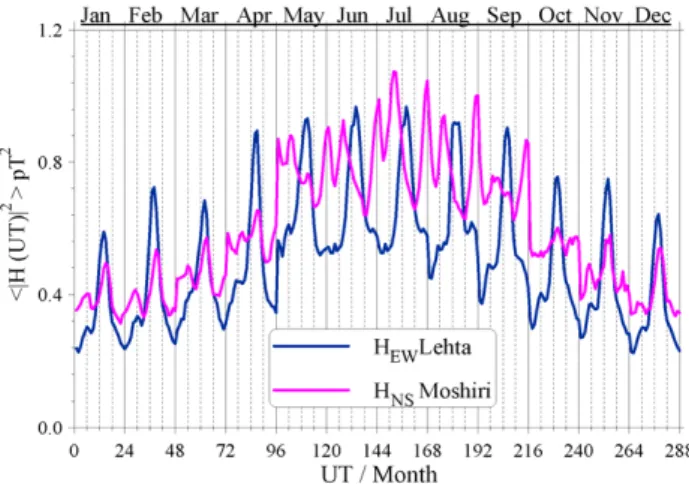
Fig. 6. Experimental data of HEW component at Lehta and the
HN Sfield at Moshiri.
source intensity or the cumulative flash number used in com-putations.
Figure 5b depicts the results of another variant of data pro-cessing when the UT modulation is directly reconstructed from the resonance intensities Q1(tL) and Q2(tL). Two
curves in Fig. 5b are in a better agreement with the cumula-tive flash number than the previous pair of Fig. 5a. Improve-ment is especially pronounced in the summer months where the recovered curves of Fig. 5a seriously deviate from each other and from the flash number. The third panel, Figure 5c, shows the geometrical average GA=√P1(tU)·P2(tU) of
the data. Again, the simple procedure proved to be efficient, and correspondence with the source intensity is as good as in plots (a) and (b). The lowest plot in Fig. 5 separately depicts the diurnal/seasonal alternations of the cumulative number of flashes.
As Fig. 5 demonstrates, patterns obtained by different schemes have much in common. All contain the typical fea-ture of an afternoon maximum in the thunderstorm intensity, the increase during summer. General reciprocity is present in the postulated source intensity. It seems that plots (b) and (c) are slightly better than plot (a). However, every curve deviates from the flash number, and we cannot state that SR intensity enables an exact derivation of the global thunder-storm activity. One may speak about definite quantitative agreement with possible deviations of±20%. Such an ac-curacy is not bad if we have in mind the global coverage and operational efficiency of the technique.
To conclude presentation of the model data, we must men-tion that SR computamen-tions were also made for two orthogo-nal horizontal magnetic field components. Similar process-ing was applied toward arbitrary combination of the fields “recorded” at Lehta and Moshiri, and the results were sim-ilar. This indicates robustness of the technique: the source intensity estimated is independent of the particular field com-ponent. This allows us to extend the above conclusion on the
arbitrary combination of resonance spectra collected at dis-tant observatories. Below, we apply the above procedures toward experimental data accumulated at Lehta and Moshiri.
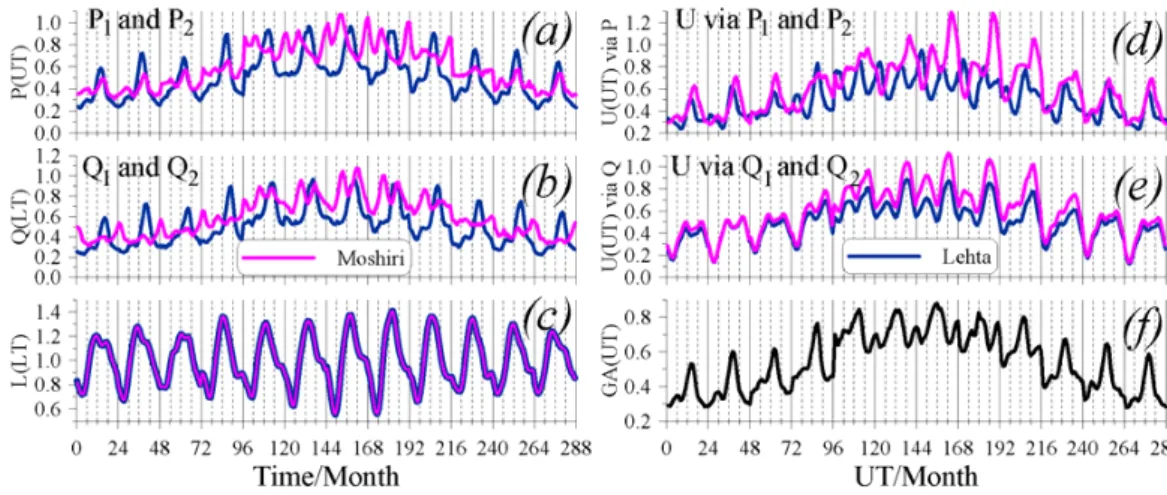
7 Processing of the experimental data
Experimental data (see Fig. 6) were collected at the Lehta and Moshiri observatories. The dark blue line depicts the UT/monthly variations of resonance intensity in the HEW
component at Lehta and the pink line depicts the HN S
Moshiri record. Experimental data continuously cover the period from January 1999 to December 2001. We use the monthly averaged diurnal variations at a site. As Fig. 6 demonstrates, diurnal patterns of Lehta and Moshiri are sim-ilar, especially in winter. Deviations appear in the interval from May to September, probably caused by a contribution from the nearby lightning strokes: the fine structure of the Moshiri record might be conditioned by thunderstorms of the South-East Asia and the Northern Australia.
Figure 7 surveys the processing results of the experiment. Plots are depicted against the time/month argument as it was done before. Plot (a) in Fig. 7 presents the initial dataP1(tU)
– Lehta (blue line) andP2(tU)– Moshiri (pink line) as the
functions of the universal time. According to Polk (1969) and Nickolaenko (1997), these plots are two independent estimates for the diurnal/seasonal alternations in the global thunderstorm activity.
Figure 7b shows the same data plotted against the local time of observatories:Q1(tL)– Lehta (blue line) andQ2(tL)
– Moshiri (pink line). Figure 7c depicts the local modulat-ing functionsL1(tL)andL2(tL)derived with the five term
Fourier expansion (4). These two functions coincide again. However, variations following from the SR measurements deviate from the model data of Fig. 4, thus indicating lim-itations of any, even sophisticated models. The local factors have patterns varying with season, and the highest modula-tion may exceed±40% level even in the cumulative SR in-tensity.
The right plots in Fig. 7 present the universal modulation factors against the UT. Figure 7d depicts functionsU1(tU)–
Lehta (blue line) andU2(tU)– Moshiri (pink line). These
were obtained by dividing the original records P1(tU)and
P2(tU)by the local modulating functionsL1(tU)andL2(tU).
Figure 7e shows the universal factors obtained by the second variant of the processing: the direct extraction from the orig-inal records (5). Figure 7f shows the geometric average of experimental data in the UT.
Fig. 7.Survey of experimental data from Lehta and Moshiri and of the local and universal modulations derived.
is important to mention a “podium” in the global lightning activity present in experiment. Owing to the podium, neither SR intensity nor the evaluated thunderstorm activity become very small (Yatsevich et al., 2006). This experimental result contradicts the expectations based on climatological percep-tions. Indeed, the global thunderstorm activity is small over the oceans. The resonance signal should decrease by a fac-tor of ten or so during the UT night when the Pacific thun-derstorms (being practically absent) become the major field source. Instead, the observed intensity reduces, but only by a factor of 2 or 3 because the experimental curves are elevated over the abscissa, as if they are placed on a “podium”. The level of such a podium increases in summer. Probably, the podium signal reflects the thunderstorm activity uniformly distributed over the globe (Yatsevich et al., 2006).
8 Conclusion
In the present paper, we extend the Sentman and Fraser (1991) technique suggested for separating the universal and the local factors in the SR intensity. We tested the tech-nique on the model resonance data relevant to the uniform Earth-ionosphere cavity with the spatial distribution of light-ing strokes based on the OTD satellite records. The Dayside Model was applied, and particular observatories were chosen at Moshiri (Japan) and Lehta (Russia).
Computations indicate that the integrated field intensity of resonance yet depends on the source distribution thus con-firming conclusion by Pechony and Price (2006). The algo-rithm we use includes the higher-order Fourier terms, so that diurnal variations acquire complicated forms that alter with the season.
The major goal was extracting the universal modulating function, which reflects alterations in the global thunder-storm activity. Three variants were used for the purpose. The first one finds and compensates the local factors in the
cumu-lative resonance intensity recorded in the universal time. The second variant directly extracts the universal factor from two records, each performed in the local time. The third one is a simple geometrical averaging of the input data presented in the UT. Computations show that all variants similarly im-prove the reciprocity to the model source intensity, but the coincidence is never achieved. Characteristic deviations are of±20%.
The same three variants of signal processing were applied toward the averaged long-term experimental data collected at Moshiri and Lehta observatories separated along the latitude and longitude by a great distance. Both local and univer-sal modulating functions were deduced from the records. A comparison of the universal variations showed their qualita-tive similarity. Results of data processing show that none of these variants allows for exact deducing the instant level of the global thunderstorm activity from the SR. The accuracy of the estimates is about±20%. The geometrical averag-ing of the SR data acquired at distant sites is the simplest technique, which provides accuracy comparable with that of more complicated Fourier expansions.
Two particular observatories were used here to illustrate the idea. Additional studies are possible comparing different pairs of existing sites. Besides, an optimal positioning might be sought for the SR observatories that monitor the global thunderstorm activity. However, these interesting points de-serve a separate treatment.
Summarizing the results of present study, we formulate the following recommendations for estimating the global thun-derstorm activity from SR records:
1. Use at least five terms in Fourier expansions of the local and global factors. These might be helpful when obtain-ing traces of the global thunderstorm centers.
3. Include the geometric averaging of cumulative intensi-ties recorded in the UT. Its closeness to theU-factors found with the Fourier expansions is a measure of accu-racy of the “output” data.
Acknowledgements. We are grateful to Sekisui Chemical Founda-tion and NiCT (R&D promoFounda-tion scheme funding internaFounda-tional joint research) for their supports.
Topical Editor U.-P. Hoppe thanks one anonymous referee for her/his help in evaluating this paper.
References
Christian, H. J., Blakeslee, R. J., Boccippio, D. J., Boeck, W. L., Buechler, D. E., Driscoll, K. T., Goodman, S. J., Hall, J. M., Koshak, W. J., Mach, D. M., and Stewart, M. F.: Global fre-quency and distribution of lightning as observed from space by the Optical Transient Detector, J. Geophys. Res., 108(D1), 4005, doi:10.1029/2002JD002347, 2003.
Hayakawa, M., Sekiguchi, M., and Nickolaenko, A. P.: Diurnal variations of electric activity of global thunderstorms deduced from OTD data, J. Atmos. Electr., 25(2), 55–68, 2005.
Nickolaenko, A. P. and Rabinowicz, L. M.: Study of the annual changes of global lightning distribution and frequency variations of the first Schumann resonance mode, J. Atmos. Terr. Phys., 57, 1345–1348, 1995.
Nickolaenko, A. P.: Modern aspects of Schumann resonance stud-ies, J. Atmos Sol.-Terr. Phy., 59, 805–816, 1997.
Nickolaenko, A. P., S´atori, G., Ziegler, V., Rabinowicz, L. M., and Kudintseva, I. G.: Parameters of global thunderstorm activity de-duced from the long-term Schumann resonance records, J. At-mos. Sol.-Terr. Phy., 60, 387–399, 1998.
Nickolaenko, A. P. and Hayakawa, M.: Resonances in the Earth-ionosphere Cavity, Kluwer Academic Publishers, Dordrecht-Boston-London, 380 pp, 2002.
Nickolaenko, A. P., Hayakawa, M., and Sekiguchi, M.: Variations in global thunderstorm activity inferred from the OTD records, Geophys. Res. Lett., 33, L06823, doi:10.1029/2005GL024884, 2006.
Pechony, O., Price, C., and Nickolaenko, A. P.: Model vari-ations of Schumann resonance based on OTD maps of the global lightning activity, J. Geophys. Res., 111, D23102, doi:10.1029/2005JD006844, 2006.
Pechony, O. and Price, C.: Schumann resonances: interpreta-tion of local intensity modulainterpreta-tions, Radio Sci., 41, RS2S05, doi:10.129/2006RS003455, 2006 (printed 42(2), 2007). Polk, C. and Fitchen, F.: Schumann resonances of the
Earth-ionosphere cavity – Extremely low frequency reception at Kingston, R.I., J. Res. Nat. Bur. Stand. U.S., Sect. D, 66, 313– 318, 1962.
Polk, C.: Relation of ELF noise and Schumann resonances to thun-derstorm activity, Planetary Electrodynamics, edited by: Coro-noti, S. and Hughes, J., vol.2, Ch.6, 55–83, Gordon and Breach, New York, 1969.
Sentman, D. D. and Fraser, B. J.: Simultaneous observation of Schumann resonances in California and Australia: evidence for intensity modulation by local height of D region, J. Geophys. Res,, 96(9), 15 973–15 984, 1991.