Amr Hany Saleh
The European Master’s Program in Computational Logic
Masters Thesis
Constraint Reasoning with Local Search for
Continuous Optimization
Dissertação para obtenção do Grau de Mestre em Logica Computicional
Orientador :
Jorge Cruz, CENTRIA, Universidade Nova de Lisboa
Júri:
Presidente: Pedro Barahona
Constraint Reasoning with Local Search for Continuous Optimization
Copyright cAmr Hany Saleh, Faculdade de Ciências e Tecnologia, Universidade Nova de Lisboa
Declaration of Authorship
I, Amr Hany Saleh, declare that this thesis titled, “Constraint Reasoning with Local Search for Continuous Optimization” and the work presented in it are my own. I confirm that:
This work was done wholly or mainly while in candidature for a research degree at
this University.
Where any part of this thesis has previously been submitted for a degree or any
other qualification at this University or any other institution, this has been clearly stated.
Where I have consulted the published work of others, this is always clearly
at-tributed.
Where I have quoted from the work of others, the source is always given. With the
exception of such quotations, this thesis is entirely my own work.
I have acknowledged all main sources of help.
Where the thesis is based on work done by myself jointly with others, I have made
clear exactly what was done by others and what I have contributed myself.
Signed:
Acknowledgements
I would like to thank and express my highest gratitude to all those who gave me the possibility to complete this thesis. Firstly, I would like to thank my supervisor, Professor Jorge Cruz for his guidance, supervision, valuable suggestions and vision he provided during the course of working on this thesis. I am also very thankful to the EMCL com-mission for giving me the chance to study in a highly acknowledged and competitive masters program like EMCL.
Abstract
Optimization is a very important field for getting the best possible value for the opti-mization function. Continuous optiopti-mization is optiopti-mization over real intervals. There are many global and local search techniques. Global search techniques try to get the global optima of the optimization problem. However, local search techniques are used more since they try to find a local minimal solution within an area of the search space.
In Continuous Constraint Satisfaction Problems (CCSP)s, constraints are viewed as relations between variables, and the computations are supported by interval analysis. The continuous constraint programming framework provides branch-and-prune algo-rithms for covering sets of solutions for the constraints with sets of interval boxes which are the Cartesian product of intervals. These algorithms begin with an initial crude cover of the feasible space (the Cartesian product of the initial variable domains) which is re-cursively refined by interleaving pruning and branching steps until a stopping criterion is satisfied.
In this work, we try to find a convenient way to use the advantages in CCSP branch-and-prune with local search of global optimization applied locally over each pruned branch of the CCSP. We apply local search techniques of continuous optimization over the pruned boxes outputted by the CCSP techniques.
We mainly use steepest descent technique with different characteristics such as penalty calculation and step length. We implement two main different local search algorithms. We use “Procure”, which is a constraint reasoning and global optimization framework, to implement our techniques, then we produce and introduce our results over a set of benchmarks.
Contents
1 Introduction 1
2 Continuous Optimization 4
2.1 Local Search Optimization . . . 6
2.1.1 Unconstrained Local Search . . . 6
2.1.2 Constrained Local Search . . . 8
2.2 Global Search Optimization . . . 10
2.2.1 Deterministic methods . . . 11
2.2.2 Meta-heuristic methods . . . 12
3 Constraint Satisfaction over Continuous Domains 14 3.1 Interval Representation and Analysis. . . 16
3.2 Constraint Propagation. . . 18
3.3 Consistency Techniques . . . 21
4 Hybrid Local Search Constraint Optimization Algorithms 23 4.1 Procure, a quick introduction . . . 25
4.2 Random Local Search . . . 27
4.3 Armijo Rule with Quadratic Penalty Steepest Descent . . . 28
4.4 Box Ratio with Separate Penalty Steepest Descent . . . 34
5 Testing and Analysis 42 5.1 First Optimization Problem: Dipigri . . . 43
5.2 Second Optimization Problem : HS108 . . . 48
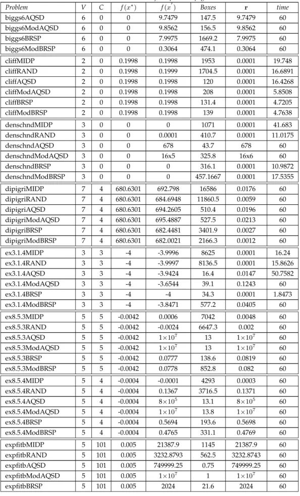
5.3 Benchmarks and Comments . . . 51
List of Figures
3.1 Standard propagation algorithm . . . 19
4.1 Pseudo code of the general CCSP-LS hybrid technique . . . 24
4.2 Example 1, simple optimization problem . . . 26
4.3 Plot of Procure example . . . 27
4.4 Random Local Search algorithm . . . 28
4.5 Steepest Descent with Quad. Penalty and Armijo. . . 29
4.6 Quadratic Penalty objective function algorithm . . . 30
4.7 Armijo rule line search algorithm . . . 31
4.8 Steepest Descent with Quad. Penalty and Armijo steps Iterations for one box 32 4.9 Modification of Steepest Descent with Quad. Penalty and Armijo . . . 33
4.10 ModifiedSteepest Descent with Quad. Penalty and Armijo steps iterations for one box . . . 33
4.11 ModifiedSteepest Descent with Quad. Penalty and Armijo steps Iterations with constraints violations . . . 33
4.12 Steepest Descent with Separate penalty and Box ratio . . . 36
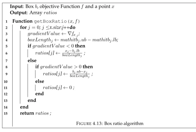
4.13 Box ratio algorithm . . . 37
4.14 Better Point algorithm . . . 38
4.15 Penalty and Violation related functions . . . 38
4.16 Box ratio steepest descent . . . 39
4.17 ModifiedBox Ratio with Separate Penalty Steepest Descent Algorithm . . 40
5.1 Example 2, Dipigri optimization problem . . . 43
5.2 Results of the five different algorithms on Dipigri Problem . . . 44
5.3 Dipigri problem algorithms convergence over time . . . 45
5.4 Dipigri problem algorithms convergence over the first 50 seconds . . . 46
5.5 Dipigri average number of branched boxes and the average time per box r= 0.01 . . . 47
LIST OF FIGURES viii
5.7 Objective function vs Penalty over time inAQSD . . . 48
5.8 Example 3, HS108 optimization problem. . . 49
5.9 Average results of the five different algorithms on HS108 problem . . . 49
5.10 HS108 problem algorithms convergence over time withr= 0.2 . . . 50
5.11 Dipigri problem algorithms convergence over the first second . . . 51
1
Introduction
In economics, engineering, scientific studies, optimization concepts and tools are used to model quantitative decisions. The aim is always to try to find the “absolute best” deci-sion which corresponds to the minimum (or maximum) of the suitable model’s objective. At the same time, a given collection of feasibility constraints might be modelled in the problem. The best decision must be satisfying these constraints. The objective in an opti-mization model expresses overall system performance, such as profit, loss, risk, or error. The constraints originate from physical, technical, economic or some other considera-tions.
An optimization problem in mathematical settings is a function representing the ob-jective of the problem over a set of variables having a domain, together with a set of constraints over these variables. Optimization is typically divided into two closely re-lated main research fields. Global optimization is the first research field. It is concerned with finding a global optimal solution for an optimization problem in a mathematical setting.
The second field is the local optimization. Local optimization is the term used for localizing the search of the optimal solution within a part of the search space of the opti-mization problem.
There are many techniques for solving optimization problems depending on the na-ture of the problem, whether it contains constraints (constrained optimization) or not (unconstrained optimization). Also depending on the aim of the search, whether to find a local optimum or global optimum.
1. INTRODUCTION
satisfied by the variables of the problem.
Constraint satisfaction problems and their techniques are divided mainly into two parts: CSP, which is the normal Constraint Satisfaction Problem (models) in discrete mathematical settings, andCCSP, which is the constraint satisfaction problem inContinuous settings. Continuous means that the domains of the variables of the problem are infinite. In this thesis, we focus more onCCSP.
With these two very brief introductions, we can observe that constraint satisfaction problems and optimization are very close in their definitions. Constraint satisfaction seeks a feasible solution, and optimization seeks an optimal solution. An optimization problem can be defined as a constraint satisfaction problem with an additional optimiza-tion funcoptimiza-tion that should be optimized along with satisfying the constraints in the prob-lem. Therefore, there is a potential of using techniques from both fields and combine them.
In the recent years, hybrid models that use optimization with constraint satisfaction appeared, as it was shown in [22]. The recent interaction between optimization and con-straint satisfaction promises to change both fields. It might be in the near future that portions of both will merge into a single problem-solving technology for discrete and continuous problems.
In this work we present two techniques that combine local search optimization with continuous constraint satisfaction. The main aim is to find a global optimal solution by dividing the search space using constraint satisfaction’s branching techniques into areas (boxes), and apply local search on these areas, keeping track of the optimal solution found so far. For each divided area in the search space, CCSPpruning techniques are applied, after which we use one of the two local search techniques, in order to find the local optimal solution of this search area.
The first technique is Armijo Rule with Quadratic Penalty Steepest Descent, and the second is Box Ratio with Separate Penalty Steepest Descent. We make comparisons be-tween these two techniques, trying to find a conclusion of which is having better timing and suitability for the given model. Moreover, we try to investigate the quality of the local search in every box, as well as the convergence and stopping strategies used.
The rest of the work is organized as follows: in chapter2, we discuss the continuous optimization techniques in mathematical settings. We present a survey on the current techniques of global and local optimization. Focusing more on the specific techniques that we use to implement our hybrid local search with continuous constraint satisfaction
(CCSP-LS)algorithms.
Afterwards, in chapter3, we show the necessary theory needed for this work about constraint satisfaction techniques over continuous domains. First, we introduce interval analysis and interval function, since the theory ofCCSPis built over these concepts. Then we discuss briefly the concept of constraint propagation that is used to prune the search space. We also discuss consistency techniques used in constraint satisfaction.
1. INTRODUCTION
CCSP-LStechniques in chaper 4. We first introduce the generic algorithm forCCSP-LS. Then, in section4.1, we give a brief overview of “Procure", the framework we use in the implementation of the algorithms. In section4.3we show the first hybrid technique and in section4.4we discuss the second technique.
In chapter 5, we show the tests we conducted on the algorithms. We run the algo-rithms over two main examples, getting information of the pruning speed and the time taken by local search techniques to find a local optimum. Moreover, we run the algo-rithms on a set of benchmarks, and show the time and comparisons between the different techniques.
2
Continuous Optimization
Optimization is important in science, mathematics and everyday problems. It dates back to 300 B.C., when Euclid considered the minimal distance between two points to be a line, and proved that a square has the greatest area among the rectangles, given the total length of edges.
In order to use optimization, we need to identify an objective to a given problem, in other words, amodel. The objective depends on certain characteristics of the system, calledvariables. The goal of the objective is to find values of the variables that optimize the objective. The variables in the given model might be constrained, meaning that they have restrictions over their domains. In this thesis, we deal with optimization in mathematical settings with variables having continuous domains.
In mathematics, an optimization problem is the minimization or maximization of an objective functionf over a vector of variablesx. This is subject to a vector of constraints cthat the variables inxmust satisfy.
An optimization problem can be written as:
min
x∈Rnf(x) subject to
(
ci(x) = 0 1≤i≤k
ci(x)≤0 k < i≤m
(2.1)
such that,
• x= (x1, x2, . . . , xn)is a vector ofnvariables of the problem.
• A functionf :Rn→Rwhich is the objective function to be minimized.
• Constraints{ci(x) = 0 |1 ≤ i ≤ k}are equality constraints over the variables in
2. CONTINUOUSOPTIMIZATION
• Constraints{ci(x) ≤ 0 |k < i≤ m}are inequality constraints over the variables
in the vectorx;
Transformation of the equations in the given model is often necessary to express an optimization problem into the standard form shown above. A very common example is changingmaximizationproblems intominimizationproblems by negating the objective functionf to−f.
An assignment of values to all variables inxrepresents an (candidate solution)option. The constraints represent limitations on theoptions. A feasible option is a solution that does not violate any constraintci. The objective function represents the costd,d=f(x).
The set of all feasible options is called the solution space. Aglobal optimum, of the prob-lem,x∗, which is also called aglobal minimizersince the standard optimization problem is a minimization problem, is a feasible solutionx∗ = (x∗1, x∗2, . . . , x∗n), whose cost is less than or equal to any solution belonging to the space of solutions.
∀x f(x∗)≤f(x) (2.2)
Normally, finding a global optimum is not as easy as finding a local optimum. A local optimum location of the problem, also noted asx∗, is a feasible solution whose cost is less than or equal to any other feasible solution belonging to a neighborhoodN, which is a subset of the search spaceS of the problem;N ⊆S. A neighborhoodN ofx∗is an open set of vectors that containsx∗.
∀xx∈N f(x∗)≤f(x) (2.3)
Most of the optimization algorithms in use today are iterative. They have a solid theo-retical basis, but the theory often allows wide latitude in the choice of certain parameters, and algorithms are often "engineered" to find suitable values for these parameters and to incorporate other heuristics.
Analysis of algorithms tackles such issues as whether the iterates can be guaranteed to converge to a solution; whether there is an upper bound on the number of iterations needed, as a function of the size or complexity of the problem; and the rate of conver-gence, particularly after the iterates enter a certain neighborhood of the solution.
Algorithmic analysis is typically worst-case in nature. It gives important indications about how the algorithm will behave in practice, but does not tell the whole story. A key aspect in solving optimization problems is the recognition of optimal solutions. Under certain assumptions, derivatives of the objective function and constraints can be used to define a set of test conditions to verify if a candidate solution is in a good place with respect to the objective function.
2. CONTINUOUSOPTIMIZATION 2.1. Local Search Optimization
functions. In the particular case of convex optimization problems, where both the objec-tive function as well as the solution space is convex, meaning all local optima are nec-essarily a global optimum. For the general case of non-convex problems, several global optimization algorithms have been proposed, some of which use techniques of integrated global local search procedures exploring the space of solutions in partitions.
Often, the variables in the model are constrained. However, some optimization prob-lems are constraints-free. This leads to dividing the optimization probprob-lems into con-strainedandunconstrainedoptimization. Moreover, optimization algorithms are mainly divided into local search algorithms, which targets finding the local optimum andglobal searchalgorithms, which targets finding theglobal optimum,
Section2.1is dedicated to local search algorithms and their strategies to take advan-tage of the characteristics of different types of optimization problems. Afterwards, in sec-tion2.2, global optimization algorithms is presented, whose main objective is to achieve global optimal solutions and therefore should introduce strategies to prevent their termi-nation in local optimal places (with values of the objective function significantly different from the global optimum).
2.1
Local Search Optimization
Local search algorithms are iterative. They begin with an initial guess, whether it is a random guess or a point supplied by the user who has knowledge about the application and the data set, and may be in a good position to choose a reasonable estimate of the solution. Beginning at the starting point, the algorithm generates a sequence of iterations to try to find points with improved estimates. The algorithm terminates when either no more progress can be made or when it seems the point in the final iteration has been approximated with sufficient accuracy.
A local search algorithm is distinguished from the others by the strategy of deciding how to move from one iteration to the next. The algorithm uses information about the objective functionf(x)and the constraintsci(x)and their derivatives, possibly combined
with information gathered at earlier stage iterations of the algorithm.
In this section, we will give an overview of the local search algorithms for uncon-strainedand forconstrainedoptimization problems. For more detailed discussion of each of these approaches, we suggest reading the classical references [50,12,17] in this area.
2.1.1 Unconstrained Local Search
Unconstrained optimization problem is defined by optimizing an objective function with no restrictions on the values of the variables involved in the function. The standard mathematical formula for the unconstrained optimization problem is:
min
2. CONTINUOUSOPTIMIZATION 2.1. Local Search Optimization
which is an instance of equation 2.1 with m = 0. There are two main strategies for unconstrained optimization;Line SearchandTrust Region.
In Line Search strategy [36], the algorithms depend on two main factors to obtain a new vectorxk+1 from the current iteration vector xk: a directiondk and a stepα. The
general mathematical form of theLine Searchalgorithm is:
xk+1 =xk+αkdk such that αk>0 (2.5)
At each iteration, a search directiondkand a positive scalarαkare decided. αkdecides
how far to move alongdk. Therefore,line searchstrategy is mainly divided into two main
criteria: the selection of thestep lengthand deciding over thedirection.
The selection of the step length always faces a trade-off between finding the best scalar value that would give a substantial reduction off, and the computation time to get such value. Therefore, line search algorithms try out a sequence of values ofαkand stop when
certain conditions are satisfied.
A very popular algorithm for calculating the step lengthis theexact line search algo-rithm which has the following formulation:
αk = min
α f(xk+αdk), (2.6)
with the following stopping condition:
f(xk+αkdk)<f(xk). (2.7)
Another popular algorithm for calculating step length is the inexact line search algo-rithm. It has the following stopping condition:
f(xk+αdk)≤f(xk) +c1α∇f⊺
kdk (2.8)
Typically,0 < c1 ≤ 1is a scalar factor. ∇fx is the vector of partial derivatives off over
the variables in the vector x, which is also called the gradient off at the pointx. The reduction inf is proportional to bothαand the directional derivative multiplied by the direction: ∇f⊺
kdk. This method is also called theArmijo rule, named after Larry Armijo
[2].
Many popular optimization algorithms are based on theline search strategy. For ex-ample, one of the very intuitive algorithms isthe steepest descentalgorithm, mentioned in [37,1]. It sets the directiondxto be the gradient of the objective function,∇f, and it has
the following formulation on obtainingxk+1fromxk:
f(xk+1) =f(xk)−αk∇fk (2.9)
Steepest descent uses the directional derivative ∇fk to get the direction of the
2. CONTINUOUSOPTIMIZATION 2.1. Local Search Optimization
problem, we take the opposite direction of the gradient−∇fk.
Other popular line search algorithms includeThe Newton,The Quasi-Newtonand Con-jugate Gradientalgorithms.
In theTrust Regionstrategy [35, 7], the collected information aboutf is used to con-struct a model functionmk, whose behavior near the current pointxkis similar to that of
the actual objective functionf. Because the modelmkmay not be a good approximation
off whenx∗ is far fromxk, we restrict the search for a minimizer ofmkto some region
around xk. We try to find a candidate stepp by approximately solving the following
subproblem:
min
p mk(xk+p) where xk+p lies inside the trust region (2.10)
Ifpdoes not give a sufficient decrease in the objective function f, then the trust region is too big. Therefore, it is shrinked and the subproblem is reevaluated. The trust region has a radius∆and the steppis normally bounded by it;||p||2≤∆. The definition of the model formkis usually a quadratic function having the following formulation:
mk(xk+p) =fk+p⊺∇fk+
1
2p
⊺B
kp, (2.11)
wherefkand∇fkare the objective function and its gradient values at the pointxk,
respec-tively.Bkis usually the second derivative offkor an approximation to it.
The trust region algorithm technique is to first choose a maximum trust-region radius
∆k, and then seek a direction and step that gets the best improvement possible subject
to this region constraint. If this step proves to be unsatisfactory, we reduce the radius measure∆kand try again.
There are several popular trust region algorithms including the Cauchy point algo-rithm, theDoglemethod and theSteihaug’s approach[45].
2.1.2 Constrained Local Search
Constrained optimization is the normal case of optimization problem, having the stan-dard minimization formulation, which we saw in equation 2.1. The set Ω of feasible points that are candidate solutions for the optimization problem2.1is defined by:
Ω ={x∈Rn|ci(x) = 0, 0≤i≤k; ci(x)≤0, k < i≤m} (2.12)
Such thatnis the number of variables in vectorx. Equation2.1can be rewritten to:
min
x∈Ωf(x) (2.13)
2. CONTINUOUSOPTIMIZATION 2.1. Local Search Optimization
Linear programming[25], which dates back at least as far as Fourier, is an important special case of constrained optimization problems for which very efficient specialized al-gorithms are available. These problems are specified by having a linear objective function
f and linear constraintsci.
In these specific problems, the contours of the objective functions are planner. There-fore, a local minimum or global minimum must lie on a vertex of the feasible set.
There are two important algorithms for linear programming: The Simplex Methodand
The Interior Point Method.
The simplex method which was developed by George Dantzig [9] moves from ver-tex to neighboring verver-tex of the feasible set, decreasing the objective function with each move, and terminating when it cannot find a neighboring vertex with a lower objective value. It mainly depends on maintaining the KarushKuhnTucker (KKT) condition and performing some operations on the feasible set if one of theKTTconditions got violated. Interior-point methods, introduced by Karmarkar [26], approach the boundary of the feasible set only in the limit. They may approach the solution either from the interior or the exterior of the feasible region, but they never lie on the boundary of this region. Each interior-point iteration is expensive to compute and can make significant progress toward the solution, while the simplex method usually requires a larger number of inexpensive iterations.
Geometrically speaking, the simplex method works its way around the boundary of the feasible polytope, testing a sequence of vertices in turn until it finds the optimal one. Interior-point methods approach the boundary of the feasible set only in the limit. They may approach the solution either from the interior or the exterior of the feasible region, but they never actually lie on the boundary of this region.
Non-Linear Constraint Optimization category is what mainly most constrained opti-mization problems classification fall under. It is an optiopti-mization problem where the ob-jective functionf or one of the constraintsci(x)are not linear.
There are many algorithms and approaches developed for solving non-linear con-straint optimization problems. However, most of them depend on transforming or sim-plifying the problem into subproblems, that have efficient algorithms to solve them.
Very popular techniques for solving non-linear constraint optimization problems are the penalty and augmented Lagrangian methods. These techniques’ idea is mainly to transform the constrained problem into unconstrained problems by applying penalty value for the constraints involved in the problem, generating a new objective function that includes these penalty values. One of the very popular algorithms is thequadratic penalty method, mentioned in [50], which adds to the objective function an additional term for every constraint in the problem. The newly obtained objective functionQ(x)has the following formula:
Q(x) =f(x) + 1
2µ
i=k
X
i=0
c2i(x) + 1
2µ
i=m
X
i=k+1
2. CONTINUOUSOPTIMIZATION 2.2. Global Search Optimization
Such that µ > 0 is the penalty parameter controlling the impact of the penalty val-ues over the obtained objective functionQ. Afterwards, we try to minimize the uncon-strained objective functionQusing the algorithms for unconstrained optimization prob-lems with a series of increasing values ofµ.
Another penalty oriented method is the augmented Lagrangian method, where we define a function that combines the properties of the quadratic penalty function of the Lagrangian function. The Lagrangian function for the standard optimization problem defined in (2.1) is defined as follows:
L(x, λ) =f(x)− i=m
X
i=0
λici(x), (2.15)
where λi is a vector of Lagrangian multipliers. This so-called augmented Lagrangian
function has the following form for equality-constrained problems:
LA(x, λ;µ) =f(x)− i=k
X
i=0
λici(x) +
µ
2
i=k
X
i=0
c2i(x) (2.16)
We try to fix the value ofλto some estimate of the optimal Lagrange multiplier vector, then fixµto a value greater than zero, then find a value ofx that approximately mini-mizesLA(x, λ;µ). The augmented Lagrangian method was first introduced by Hestences
[21] and Powell [39]. It was also mentioned in [51].
From the other several algorithms available for non-linear constraint optimization problems, there are also the sequential quadratic programming; introduced in late 1970’s, described in [5]. It can be used both in line search and trust-region frameworks, and it is appropriate for both small or large problems. Here the idea is to model the original prob-lem by a quadratic subprobprob-lem at each iteration, and to define the search direction as the solution of this subproblem. The objective in this subproblem is an approximation of the Lagrangian function and the constraints are linearizations of the original constraints. The new iteration is obtained by searching along this direction until a certain merit function is decreased. Sequential quadratic programming methods have proved to be effective in practice. They are the basis of some of the best software for solving both small and large constrained optimization problems. They typically require fewer function evalua-tions than some of the other methods, at the expense of solving a relatively complicated quadratic subproblem at each iteration.
2.2
Global Search Optimization
2. CONTINUOUSOPTIMIZATION 2.2. Global Search Optimization
One class of methods for solving the global optimization problem are the determin-istic methods. One of the techniques of the determindetermin-istic methods, in other words: exact methods, is to use a process of subdividing the feasible region and using information about the objective function to obtain a lower bound on the objective in that region, lead-ing to the branch-and-bound algorithm. These methods can provide assurance of the quality of the solution found.
There is also another class of methods which depends on meta-heuristics. However, this class of methods does not guarantee the quality of the solution.
In this section, we will give a brief introduction to the the different classes of global optimization algorithms.
2.2.1 Deterministic methods
Deterministic algorithms for continuous global optimization problems guarantee that by the termination of it to have found at least one global minimum of the given optimization problem. However, since the domains of the variables are continuous, the algorithms are more likely to take a very long time to find a global minimum.
There are several deterministic global optimization algorithms. We will discuss the
branch-and-boundalgorithms, discussed in [19,27]. These algorithms are considered the most popular deterministic global optimization methods. To apply branch-and-bound, one must have a means of computing a lower bound on an instance of the optimization problem and a means of dividing the feasible region of a problem to create smaller sub-problems. There must also be a way to compute an upper bound (feasible solution) for at least some instances; for practical purposes, it should be possible to compute upper bounds for some set of nontrivial feasible regions. The method starts by considering the original problem with the complete feasible region, which is called theroot problem.
The lower-bounding and upper-bounding procedures are applied to the root prob-lem. If the bounds match, then an optimal solution has been found and the procedure terminates. Otherwise, the feasible region is divided into two or more regions, each strict subregions of the original, which together cover the whole feasible region, these subprob-lems partition the feasible region. These subprobsubprob-lems become children of the root search node.
2. CONTINUOUSOPTIMIZATION 2.2. Global Search Optimization
[32]. In Bayesian search algorithms, techniques for modeling data by Bayesian networks are developed to estimate the joint distribution of promising solutions. Moreover, enu-merative methods which, as its name suggests, enumerates all possible solutions. How-ever, since the domains of the variables are infinite in continuous domains, a set of ap-proximates of all the possible solution is used. This strategy is applicable to small sized problems which have a small feasible area.
2.2.2 Meta-heuristic methods
Meta-heuristic methods do not guarantee to obtain the global optimum solution for the optimization problem. However, the techniques followed by these methods make them reach a solution which is very close to the local optimum or even the global optimum itself. Moreover, the meta-heuristic methods are very competitive to the deterministic methods, because it takes much less time to compute and give very good results. Meta-heuristic methods are discussed in details in [16].
Local search methods can get stuck in a local minimum, where no improving neigh-bors are available. A simple modification consists of iterating calls to the local search routine, each time starting from a different initial configuration. This is called repeated local search, and implies that the knowledge obtained during the previous local search phases is not used. Learning implies that the previous history, for example the mem-ory about the previously found local minima, is mined to produce better starting points for local search. Iterated Local Searchalgorithm, described in [29], is based on building a sequence of locally optimal solutions by perturbing the current local minimum and applying local search after starting from the modified solution.
Another meta-heuristic method isSimulated Annealing; discussed in [47,11] which is a random-search technique which exploits an analogy between the way in which a metal cools and freezes into a minimum energy crystalline structure (the annealing process), and the search for a minimum in a more general system. The major advantage over other methods is an ability to avoid becoming trapped in local minima.
The algorithm employs a random search, which not only accepts changes that de-crease the objective function, but also some changes that inde-crease it. The latter are ac-cepted with a probability given by a function of the increase in the objective function and a control parameter, known as the system ”temperature". The temperature is decreasing (cooling) slowly according to a predefined schedule, in order to decrease the probability of accepting worst solutions as exploring the space of solutions.
There is also theTabu Searchmethod, discussed in [6]. The idea of this popular meta-heuristic algorithm is to block the search moves to points already visited in the search space, or just block it for the nextkiterates. The main use of the tabu search algorithm is in discrete optimization problems, but it can also be extended to handle continuous global optimization problems.
2. CONTINUOUSOPTIMIZATION 2.2. Global Search Optimization
natural selection and survival of the fittest in the biological world. EA differ from more traditional optimization techniques in that they involve a search from a “population" of solutions, not from a single point. Each iteration of an EA involves a competitive selec-tion that weeds out poor soluselec-tions. The soluselec-tions with high “fitness" are “recombined" with other solutions by swapping parts of a solution with another. Solutions are also “mutated" by making a small change to a single element of the solution. Recombination and mutation are used to generate new solutions that are biased towards regions of the space for which good solutions have already been seen.
3
Constraint Satisfaction over
Continuous Domains
Constraints are the way to specify a relation that must hold between two or more vari-ables. This is done by restricting the possible values that these variables can have. In mathematics, constraints are accurately specified relations between variables. AConstraint SatistfactionProblem (CSP) is a model with variables, such that each variable is ranging over a domain. Constraints over these variables restrict the respective domain values that can be assigned to the variables. The aim of any CSP is to give a value for each variable that does not violate any of the constraints. CSP was introduced in early seventies in [49, 33, 30]. The following definition is the formal definition of a constraint, mentioned in [8]1:
Definition 3.1. A constraintcis a pair(s, ρ), wheresis a tuple ofmvariables< x1, x2, . . . , xm >,
the constraint scope, andρis a relation of aritym, the constraint relation. The relationρ is a subset of the set of allm-tuples of elements from the Cartesian productD1 ×D2 ×
· · · ×Dm whereDiis the domain of the variablexi:
ρ⊆ {< d1, d2, . . . , dm>|d1∈D1, d2 ∈D2, . . . , dm∈Dm} (3.1)
The tuples inρare the tuples that allow the satisfaction ofc. The arity ofcism, which is the length of the tuples inρ.
3. CONSTRAINTSATISFACTION OVERCONTINUOUSDOMAINS
The constraints in a CSP can be represented explicitly, by stating all the allowed com-binations of variables’ values of every constraintc in the CSP. They can also be repre-sented implicitly by means of mathematical expressions or procedures that can be com-puted in order to determine these combinations.
Definition 3.2. A CSP is a triple P = (X, D, C) where X is a tuple of n variables < x1, x2, . . . , xn>,Dis the Cartesian product of the respective domainsD1×D2× · · · ×Dn,
i.e. each variablexiranges over the domainDi, andCis a finite set of constraints where
the elements of the scope of each constraint are all elements ofX.
A solution to a CSP is a tuple of values, each value assigned to a variable, such that it satisfies all the constraints inC.
Definition 3.3. A solution to the CSPP = (X, D, C)is a tupled∈ Dthat satisfies each constraintc∈C, that is:
dis a solution ofP iff2∀ci=(si,ρi)∈C d∈ρi
A CSP may have one, several, or no solutions. In practice, the modeling of a problem as a CSP is embedded in a larger decision process. Depending on this decision process it may be desirable to determine whether a solution exists, meaning that the overall CSP is consistent. The process might also try to find a solution for the CSP, a set of whole solutions to the CSP or an optimal solution for an objective function (to turn into an optimization problem).
Definition 3.4. A CSP,P = (X, D, C) is consistent iff it has at least one solution: P is consistent iff∃d∈Dsuch thatdis a solution ofP.
There are several ways to solve a CSP. The main strategy is to use each constraint separately and try to eliminate values of the variables that guaranteedly can not satisfy it (and consequently, no valid solution is lost). This is calledconstraint propagation. This decreases the search space where the algorithm is looking for a solution. We discuss constraint propagation more in section3.2.
Numeric CSP’s, introduced by Davis in [10], are the extension of the CSP to include variables over continuous domains, since earlier CSPs were only devoted for problems including variables over finite domains.
Definition 3.5. A NCSP is a CSPP = (X, D, C)where: i)∀Di∈DDi ⊆ Z ∨Di⊆R
ii)∀(s,ρ)∈C ρis defined as a numeric relation between the variables ofs.
In NCSP, constraints have to be expressed implicitly, as a numeric relation between the variables, since the explicit representation of the constraints might be infinite.
Continuous CSPs are a special class of NSCP where the shape of constraints expres-sion has to be specific. This is the definition of CCSP based on [41].
3. CONSTRAINTSATISFACTION OVERCONTINUOUSDOMAINS 3.1. Interval Representation and Analysis
Definition 3.6. CCSP is a CSP,P = (X, D, C)where each domain is an interval ofRand each constraint relation is defined as a numerical equality or inequality:
i)D=< D1, . . . , Dn>whereDiis a real interval(1≤i≤n).
ii)∀c∈C cis defined asec⋄0whereecis a real expression and⋄ ∈ {≤,=,≥}.
In a CCSP, the domains associated with the variables are intervals which are infinite sets of real numbers. However, to represent infinite sets of real numbers on a computer system, several techniques were developed. In section3.1we talk about how CCSP do-mains are represented and operations that can be done over them. Afterwards, in section 3.2, we discuss the concept of constraint propagation and the elimination of inconsistent values. In section3.3, we discuss popular consistency techniques for CCSPs.
3.1
Interval Representation and Analysis
In order to represent a continuous domain in a computer system,F-numbers were pre-sented, as defined in several publications [28,3,46].
Definition 3.7. Let F be a subset of Rcontaining the real number 0 as well as finitely many other reals, and two elements (not reals) denoted by−∞,+∞:
F=r0, . . . , rn∪ {−∞,+∞} with 0∈ {r0, . . . , rn} ⊂R
The elements ofFare calledF-numbers.
The elements ofFare totally ordered wrt3R. Moreover, iff is anF-number, then f−
andf+are twoF-numbers which are directly before and afterf inFwrt the total order. With the introduction of F-number,F-interval is introduced, which is the subset of real intervals that can be represented by a particular machine as the set of real intervals bounded byF-numbers.
Definition 3.8. AnF-intervalis a real interval∅or< a..b >whereaandbareF-numbers. In particular, ifb=aorb=a+then< a..b >is a canonicalF-interval.
To express a set of variables’ domains in a CCSP, we use the notion of a box. AnF-box
is an extension to the concept ofF-interval, with several dimensions.
Definition 3.9. AF-box BFwith arity nis the Cartesian product of nF-intervals and is denoted by< IF1, . . . , IFn>where eachIFiis anF-interval:
BF={< r1, r2, . . . , rm > | r1 ∈IF1, r2∈IF2, . . . , rn∈IFn}.
In particular, if all theF-intervalsIFiare canonical, thenBF is a canonicalF-box.
Interval analysis, introduced in [34], is very important for CCSP in order to be able to eliminate inconsistent solutions. It is used in many proofs of the soundness of constraint propagation techniques. Interval analysis is based on interval arithmetic, which is an extension of real arithmetic for real intervals.
3. CONSTRAINTSATISFACTION OVERCONTINUOUSDOMAINS 3.1. Interval Representation and Analysis
Interval arithmetic redefines the basic real arithmetic, like sum, difference, product and quotient. We define the basic interval arithmetic operators as follows:
Definition 3.10. LetI1 andI2 be two real intervals. The basic arithmetic operations on intervals are defined by:
I1ΦI2 ={r1Φr2 |1∈I1∧r2∈I2} with Φ∈ {+,−,×, /}
except that I1/I2 is not defined if0∈I2. (3.2)
To define the basic operators, let[a..b]and[c..d]be two real intervals. Therefore:
• [a..b] + [c..d] = [a+c..b+d]
• [a..b]−[c..d] = [a−d..b−c]
• [a..b]×[c..d] = [min(ac, cd, bc, bd)..max(ac, cd, bc, bd)]
• [a..b/[c..d] = [a..b]×[1/d..1/c] if0∈/ [c..d]
Most algebraic properties in the case of real arithmetic, such as commutativity and associativity hold also in interval arithmetic, However, in distributivity, if we haveI1, I2 andI3intervals then the sub-distributivity law becomes:
I1×(I2+I3)⊆I1×I2+I1×I3 (3.3)
According to [34], interval analysis and evaluations are sound and correct. This soundness is one of the major contributions to the interval constraints framework. Since a function can be expressed in different equivalent expressions, interval evaluations of these expressions may yield different interval results. However, the soundness of inter-val arithmetic guarantees that all the output interinter-vals contain the intended results for the function. We show the formal definition of interval expressions and the representation of interval function next.
Definition 3.11. An expressionEis an inductive structure defined in the following way: (i) a constant is an expression;
(ii) a variable is an expression;
(iii) ifE1, . . . , Emare expressions andφis am-ary basic operator thenφ(E1, . . . , Em)is an
expression; a real expression is an expression with real constants, real-valued variables and real operators. An interval expression is an expression with real interval constants, real interval valued variables and interval operators.
3. CONSTRAINTSATISFACTION OVERCONTINUOUSDOMAINS 3.2. Constraint Propagation
3.2
Constraint Propagation
In a CCSPP = (X, C, D), the initial domains of variables inXare infinite sets, since they are real intervals. The whole domain of the problem obtained by the power set ofDis also infinite. Therefore, solving a CCSP is theoretically over infinite space. However, due to the computer’s limitation to represent real numbers, approximation usingF-numbers is used. The search starts considering the smallestF-box enclosingD. Then a pruning step starts, which tries to remove inconsistent options from the box. Which results in returning a newF-box or a union ofF-boxes.
The pruning step consists of reducing anF-box (or a union ofF-boxes)Ato a smaller
F-box (or a union ofF-boxes)A′. The pruning algorithm must make sure that there are no potential solutions removed from the original box. Nonetheless, the filtering algorithm may be unable to prune some inconsistencies due to the limited representation power.
The branching step comes after pruning, which consists of dividing the pruned F -box intom smallerF-boxes, such that, the union of themF-boxes must be the same as the originalF-box. Then afterwards pruning is applied to the divided boxes, trying to remove further options which are not solutions.
The technique described before is called branch and prune. For the sake of simplifi-cation of the domain’s representation, most solving strategies impose that only the single F-boxes should be presented (as opposed to a union of F-boxes). In that sense, prun-ing corresponds to narrowprun-ing the originalF-box into a smaller one, where the lengths of someF-intervals are decreased by some filtering algorithms (or if it became empty, prov-ing the originalF-box to be inconsistent). The branching step usually consists of splitting the originalF-box into two smallerF-boxes by splitting one of the original variable do-mains around anF-number, which is in most algorithms theF-number representing the mid-value of theF-interval of its domain.
The filtering algorithms are used for pruning the variable domains. They are based on constraint propagation techniques. The propagation process is described as a succes-sive pruning to the variables domains’. This is done by applyingnarrowing functions associated to the constraints of the CCSP. Evaluation of the narrowing functions is done by algorithms that take advantage of the techniques of interval analysis.
In the propagation algorithm, a narrowing function is the mapping between elements in a domain: A, andA′, such that the new elements inA′ are obtained by eliminating some value fromA. In the following, the definition of the narrowing function is shown.
Definition 3.12. LetP = (X, D, C)be a CCSP. Anarrowing functionN F associated with a constraintc = (s, ρ)(withc ∈C) is a mapping between elements of2D (Domain
N F ⊆
2D andCodomain
NF ⊆ 2D)with the following properties (where A is any element of
DomainNF):
P1)N F(A)⊆A(contractance)
3. CONSTRAINTSATISFACTION OVERCONTINUOUSDOMAINS 3.2. Constraint Propagation
From propertyP1, it is assured that the new domainN F(A)is smaller thanA. More-over, with propertyP2, the narrowing function does not remove any valid solution for the CCSP.
A narrowing function has to be monotonic and idempotent according to [38] or at least monotonic according to [4].
Definition 3.13. LetP = (X, D, C)be a CCSP. Let N F be anarrowing function asso-ciated with a constraintC. Let A1 andA2 be any two elements of DomainN F. N F is
respectively monotonic and idempotent iff the following properties hold: P3)A1 ⊆A2→N F(A1)⊆N F(A2)(monotonicity)
P4)N F(N F(A1)) =N F(A1)(idempotency)
Input: setQof narrowing functions, a boxB ⊆D Output: a boxB′ ⊆B
1 functionprune(Q,B) 2 S ← ∅;
3 whileQ6=∅do 4 chooseN F ∈Q; 5 B′ ←N F(B); 6 ifB′ =∅then 7 return∅; 8 end
9 P ← {N F′ ∈S:∃x∈RelevantN F′B[x]6=B ′[x]};
10 Q←Q∪P; 11 S ←S\P; 12 ifB′ =B then 13 Q←Q\{N F}; 14 S ←S∪ {N F}; 15 end
16 B ←B′; 17 end
18 returnB;
FIGURE3.1: Standard propagation algorithm
The standard propagation algorithm in figure 3.1takes two arguments: Q, which is the set of all narrowing functions associated with the constraints in the CCSP, and B, which is a subset of the power-set of the domains of the CCSP.
In the beginning of the algorithm, the setSis initialized to the empty set. Scontains the narrowing functions for which B is necessarily a fixed-point. Then, until Qis not empty, it starts applying the narrowing functions inQby selecting a narrowing function N F, and applying it toB to getB′. Then it checks: if the domain ofB′ is empty, then there is no solution for the problem returning an empty set.
3. CONSTRAINTSATISFACTION OVERCONTINUOUSDOMAINS 3.2. Constraint Propagation
which are the narrowing functions with relevant variables whose domains were changed by applyingN F toB, are moved fromStoQto be applied again onB. Moreover, ifB′is a fixed point forB; meaningB =B′, thenN F is moved toS. Then finallyB is updated with the values inB′ and the loop repeats again.
Many types of narrowing functions have been developed that follows the monotonic-ity and idempotency rules. There are many techniques to associate narrowing functions to the constraints of a CCSP.
One important technique is theconstraint decomposition method[24,44], mentioned in [8]. It is based on the transformation of complex constraints into an equivalent set of primitive constraints that can be solved with respect to each variable.
First we decompose the set of original constraints into a set of primitive constraints possibly by adding new variables. For example, the complex constraint(x2−x1)2×x1= 1 is decomposed into the primitive constraints:{x3 =x2−x1,x4 =x3,x4×x1 = 1}with the addition of the two new variablesx3 andx4.
The next step of the constraint decomposition method is to solve algebraically each primitive constraint wrt. each variable in the scope and to define an interval function en-closing the respective projection function. This is always possible because the constraints are primitive. However, an extra care must be taken due to the in-definition of some real expressions for particular real-valued combinations.
For example the primitive constraint x3 = x2 −x1 yeilds the following narrowing functions for reducing the domains of each variable:
• N F1(I1)→(I2−I3)∩I1.
• N F2(I2)→(I3+I1)∩I2.
• N F3(I3)→(I2−I1)∩I3.
There are several other narrowing functions like the Newton Method [3], and several modifications to the decomposition methods [24] and the Newton methods [46].
3. CONSTRAINTSATISFACTION OVERCONTINUOUSDOMAINS 3.3. Consistency Techniques
3.3
Consistency Techniques
The fixed-points of a set of narrowing functions associated with a constraintc character-ize a local property enforced among the variablesx1, x2, . . . , xn of the constraint scope.
Such property is calledlocal consistency. It mainly depends on these narrowing functions which are associated with only one constraint. Moreover, it defines the value combina-tions that are not removed from the variables. Local consistency is a partial consistency, which means that when it is imposed on a CCSP problem, it does not remove all the inconsistent combinations between its variables.
The local consistencies that are in use for the CCSP is a modification of the arc-consistency which is a local arc-consistency mainly used for CSP over finite domains and was introduced in [30]. Arc-consistent constraints are the constraints for which each value in the variables involved in the constraint has a consistent value with the other variables’ values of the constraints. The definition of arc-consistency is as follows.
Definition 3.14. LetP = (X, D, C) be a CSP. Letc = (s, ρ)be a constraint of theCSP. LetAbe an element of the power set ofD(A∈2D). The constraintcis arc-consistent wrt
A iff:
∀xi∈s∀di∈A[xi]∃d∈A[s](d[xi] =di∧d∈ρ)
Arc consistency can not be enforced with CCSP since the domains of the variables in the problem are infinite, and the machine has a memory limitation. Therefore, the real values are approximated into canonicalF-interval. The best approximation of arc-consistency wrt a set of real-valued combinations is the set approximation of each vari-able domain.
This is the idea of theinterval-consistency[24,44]. A constraint is interval-consistent wrt a set of value combinations iff for each canonicalF-interval representing a variable sub-domain there is a value combination satisfying the constraint. Interval-consistency has the following formal definition.
Definition 3.15. LetP = (X, D, C)be a CCSP. Letc= (s, ρ)be a constraint of the CCSP
(c∈C). Let A be an element of the power set ofD(A∈2D). The constraintcis
interval-consistent wrt A iff:∀xi∈s∀[a..a+]⊆A[xi]∃d∈A[s](d[xi]∈(a..a
+)∧d∈ρ)
∧ ∀[a]⊆A[xi]∃d∈A[s] (d[xi]∈(a
−..a+)∧d∈ρ)(whereais anF-number).
Interval-consistency can only be enforced on primitive constraints where the set ap-proximation of the projection function can be obtained using interval arithmetic. More-over, according to [24], in practice, the enforcement of interval-consistency can be applied only to small problems.
Several other kinds of local consistencies were developed. For example, the Hull-consistency[28], and theBox-consistency [3] that are variants of arc-consistency enforced only on the bounds of each variable.
3. CONSTRAINTSATISFACTION OVERCONTINUOUSDOMAINS 3.3. Consistency Techniques
4
Hybrid Local Search Constraint
Optimization Algorithms
After introducing continuous optimization in chapter 2 and continuous constraint sat-isfaction in chapter 3, we introduce our main work, in which we combine techniques of continuous optimization problems, whether constrained or unconstrained, with the branch-and-bound algorithms of CCSP.
In recent years, there has been a lot of research done in the field of hybrid constraint programming and hybrid constraints with local search [43]. This research is focusing mainly on constraints over finite domains [13]. There are many frameworks developed for constraint programming with the option of using local search techniques to satisfy the problem. One of the most famous frameworks which is mainly developed for CSP over finite domains is Comet [20].
In this thesis, we discuss the combination of branch-and-bound technique that is used to propagate constraints and solve CCSP, with continuous local search over the branched and pruned boxes of the CCSP. When solving an optimization problem, trying to get the global minimum, constraint propagation techniques are used to prune the domains of the variables in the problem after branching the search space into several boxes. We use continuous local search techniques over every box, trying to get a local minimum within that box. By comparing the results obtained for the local minima of each box, we can keep track of the minimal “local minimum”, which is the local minimum which has the lowest value found. Therefore, we get an estimate of the global minimum of the problem over the search space explored.
4. HYBRIDLOCALSEARCHCONSTRAINTOPTIMIZATIONALGORITHMS
algorithm takes a CCSP with an optimization functionf. In other words, it takes a con-strained optimization problem with the functionf that will be minimized, and a setCof constraints that are transformed into the form of constraints, appearing in the standard optimization problem in equation2.1.
In line 1, B is a set of boxes which is initialized with the initial box for the branch and prune algorithm. Afterwards, in lines2and3we initialize the variables where the minimal objective function value and the minimal local point found will be stored.1 A loop starts in line 4 until B is empty. In line 5, a box b is selected from B according to a selection criterion. This criterion selects b with the highest potential of finding a better local minimum. Branching is applied on the selected boxb, creating a set of boxes
{b1, . . . , bn}. Then another loop starts for every boxbi, starting by pruning the boxbiin
line8.
Input: A continuous optimization ProblemP with the functionf (which can also be a CCSP with an objective function)
Output: a pointx, the global minimum found so far.
1 B ←{(Initial boxb)}; 2 minimalP oint←NULL; 3 minimalV alue← ∞; 4 whileBis not emptydo
5 b← B.takeBox();
6 {b1, . . . , bn}=b.branch();; 7 foreachbi ∈ {b1, . . . , bn}do 8 bi.prune();
9 ifbi is not emptythen
10 <succeed, point>←applyLocalSearch(bi); 11 ifsucceed==truethen
12 value←f(point);
13 ifboxV alue < minimalV aluethen 14 minimalV alue←value; 15 minimalP oint←point;
16 end
17 end
18 ifstopping criteria reachedthen 19 returnminimalP oint;
20 end
21 addbitoB; 22 end
23 end
24 end
25 returnminimalP oint;
FIGURE4.1: Pseudo code of the general CCSP-LS hybrid technique
Afterwards, an emptiness check is applied onbi in line9. Ifbi is not empty, the local
4. HYBRIDLOCALSEARCHCONSTRAINTOPTIMIZATIONALGORITHMS 4.1. Procure, a quick introduction
search optimization will be applied within the box, taking into consideration that some of the local search algorithms we discuss will always maintain the bounds of the box. Others have the option of trying to get an even better optimal point by going out of the bounds of the boxbi.
The applyLocalSearch(bi) algorithm returns the pair<succeed, point>. The first
parameter in the pair is a boolean variable which is true if the algorithm succeeded to find a local minimum in thebi, andfalseotherwise. Ifsucceedistrue, then the box local
minimum is saved inpoint, and its objective function value is calculated and saved in value. Then thevalueis checked if it has the minimal value off so far. If that is the case, minimalV alueandminimalP ontare updated as it is shown in lines14and15.
At the end of every iteration, a stopping criterion is checked. Many criteria can be used, such as the difference between the lower bound of the objective function interval evaluated by interval arithmetics to the minimaV alue. If the stopping criteria is not reached,biis added toB.
We will useProcure[42], which is a probabilistic continuous domain constraint frame-work, for the implementation for our algorithms and obtaining the results. We will dis-cuss in brief howProcureworks in section4.1.
In section4.2, we implemented a random search algorithm for the sake of comparison with the local search algorithms. In later sections, sec. 4.3and4.4, we will discuss two local search algorithms we implemented with the logic that supports it. These two algo-rithms depend on the concept of the steepest descent local search. However, they have different step length calculation and penalty functions.
4.1
Procure, a quick introduction
All the algorithms we propose and investigate in this work are implemented using Pro-cure. Procure is a probabilistic continuous domain constraint framework which is built overRealPaver[18], which is an interval-based solver. Procure is developed by the Cen-tria group at the new University of Lisbon. Using theC++programming language and following an object oriented design, this solver provides a set of useful continuous con-straint methods, and its design makes it easily extensible.
Procure provides many mathematical methods for calculation, such as calculating the derivative of a function and partial derivatives. It uses branch-and-bound algorithms for constraint propagation. Moreover, with the modularity provided with it, the simplicity of changing the search algorithm within the branched boxes comes in handy.
It implements the general CCSP-LS algorithm that was shown in figure4.1. However, it does not use the local search algorithm over every processed (branched and pruned) box. What it simply does, is that it takes themid-pointsover all intervals of the variables in the branched box and return them as the point.
4. HYBRIDLOCALSEARCHCONSTRAINTOPTIMIZATIONALGORITHMS 4.1. Procure, a quick introduction
1 vector<Procure::Var> x(1);
2 Problem prob(x,{{-3,20}},{x[0] >= 0 },20 + x[0] * sin(x[0]) );
FIGURE4.2: Example 1, simple optimization problem
interval disclosure off for each box inBand maintain the ordering ofBascendingly with respect to the boxes’ lower bounds.
Moreover, when a problem is passed to Procure to find the global minimum, an im-plicit constraintcobj, shown in equation4.1, is added to the set of constraintsC of the
optimization problem. cobj makes sure that the new local minimum found by the
algo-rithm is having a lower objective value than the current local minimum. cobj also helps
in pruning the set of boxesB. From this set we remove the boxes that do not have any potential of finding the global minimum, meaning the boxes having a lower bound with a higher value than the local minimum found so far. Assume the setB has the boxes b1, . . . , bn. cobj imposes that the objective function value of the lower bound (LB) ofbi is
less than or equal to the objective function value of the minimal point (minimalV alue). cobjis updated whenever theminimalV alueis changed.
cobj =f(x)≤minimalV alue. (4.1)
In order to solve an optimization problem, in addition to the optimization function
f, we specify the variables X, the initial domains Dand the constraints C. Figure4.2 shows an example of an optimization function which is written in Procure syntax. This example will be used throughout this chapter to make comparisons with different search algorithms.
Figure4.2shows an optimization problem with one variablex[0], for simplicity, let’s call itx.xhas the initial domain of[−3,20]with one constraint in the system, that isx≥0. The optimization function is20 +x×sin(x), that we want to minimize. In figure4.3, the minimization function is presented. There are four local minima in the feasible area of the problem:
• x= 0withf(x) = 20.
• x≈4.99withf(x) = 15.185.
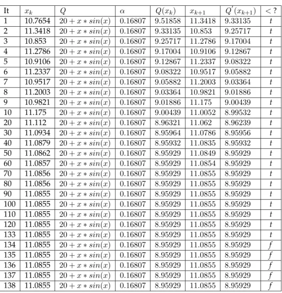
• x≈11.0855withf(x) = 8.95929.
• x≈17.3364withf(x) = 2.6924, which is also the global minimum.
4. HYBRIDLOCALSEARCHCONSTRAINTOPTIMIZATIONALGORITHMS 4.2. Random Local Search
0 5 10 15 20 25 30 35 40
0 5 10 15 20
f(x)
x
20 +xsin(x)
FIGURE4.3: Plot of Procure example
4.2
Random Local Search
In this local search algorithm, we use a completely random selection algorithm for obtain-ing a pointxfrom a boxb. Simply by taking the current boxbas an input, we randomly choosex, and then check whether it is in the feasible area of the problem. Ifxis feasible, the search terminates, andxis returned. On the other hand, if this is not the case, then a new random point is obtained. This process will continue until the maximum number of restartsis reached. If the restarts number is reached, then the algorithm fails to find any feasible point in its random search and terminates.
The local search algorithm which appears in figure4.4does what is mentioned earlier, and it returns the pair <succeed, point>. If the algorithm succeeded to find a feasible pointx, then succeedis set totrueand thepointtakes the obtained point. Otherwise, it returns<false,NULL>.
With the random local search, the time of solving an optimization problem is varied over a long time. Therefore, when we get to test this algorithm, we take an average of five runs of the problem and get the average timing.
In the problem that appeared in figure4.2. We ran the problem five times using the local search algorithm. It took an average of 0.07 seconds which is the same time of the mid-point algorithm. Most of the search space is in the feasible area. This results in most of the selected random points being feasible. This allows the branching to go faster, removing all the boxes that do not satisfy the global constraintcobj. Moreover, the
4. HYBRIDLOCALSEARCHCONSTRAINTOPTIMIZATIONALGORITHMS 4.3. Armijo Rule with Quadratic Penalty Steepest Descent
Input: a boxb
Output: A pair<Bool, P oint>
1 restarts←50;
2 fori←1torestartsdo
3 x← random point in b; 4 ifxis feasiblethen 5 return<true,x>; 6 end
7 end
8 return(false,NULL);
FIGURE4.4: Random Local Search algorithm
4.3
Armijo Rule with Quadratic Penalty Steepest Descent
In this local search algorithm, we use the steepest descent method for obtaining a new pointxk+1fromxk. Steepest descent algorithm is mentioned in section2.9.
There are two main options for implementing this algorithm: how to represent the constraints and how to select the step length. Constraints are presented in the problem using the quadratic penalty method. In other words, the count of the penalty caused by violating the constraints in the system is added to the value of the overall objective func-tion. This is done by changing the objective functionf toQ, whereQ takes into account the number and amount of violations in every constraint. The technique of quadratic penalty function is discussed in2.1.2, equation2.14.
The selection of the step lengthαkwith respect to the directiondxis determined by the Armijo rule, as shown in equation2.8. The algorithm’s stopping criteria mainly depends on the iterative settings of the algorithm. A counter is set to a numberm, then by the end of every iteration the boolean valueQ(xk+1) ≥Q(xk)is checked. The counter decreases
whenever this check is true, and resets when it is false. If formconsecutive iterations the check succeeded, the algorithm terminates, returningxk.
The main idea of this algorithm is that when the violated constraints are added as a penalty in the original objective functionf to obtainQ, then using the steepest descent in the decreasing direction ofQ, the penalty value ofxk+1is going to be less than that ofxk.
Figure 4.5 shows the algorithm with the stopping counter stops mentioned earlier. The input is a boxbwith a vectorx ofnvariables. The algorithm tries to obtain a local minimum insideb with respect to the newly obtained objective functionQ. It returns a pair<succeed, point>.succeedistrueif the algorithm found a local minimum, and it sets pointto this local minimum point. It returnsfalseif it did not succeed in finding a local minimum.
The algorithm starts by setting the restarts number, which in this case is50. Then with every restart,xkis set to be a random point inb. A stopping flag which is set to5acts as
4. HYBRIDLOCALSEARCHCONSTRAINTOPTIMIZATIONALGORITHMS 4.3. Armijo Rule with Quadratic Penalty Steepest Descent
the next five runs, the search stops. The variableµis set to1.
Afterwards, in every iteration of the local search, a new objective function Q is cal-culated using the functiongetQuadPenaltyFunction(f,xk,µ) which will be discussed
later. In addition to calculatingQ, the step ratios are calculated for every variable in b. This is done using the functiongetArmijoSteps(Q,xk) that returns an array of ratios;
a ratio for each variable.
Input: a boxb
Output: A pair<Bool, P oint>
Result: Getting a local minimum in a boxb
1 restarts←50;
2 fori←1torestartsdo
3 xk← random point in b; 4 stop←5;
5 µ←1;
6 whilestop≥0do
7 Q ←getQuadPenaltyFunction(f,xk,µ); 8 Steps←getArmijoSteps(Q,xk);
9 forj ←1tondo /*n is number of variables inxk*/
10 x(k+1).j←xk.j−Steps[j]× ∇Qj ; 11 end
12 Q′ ←getQuadPenaltyFunction(f,xk+1,µ);
13 ifQ′(xk+1)≤Q(xk)then 14 \ ∗Modification Here∗ \ 15 xk←xk+1;
16 stop←5; 17 µ←1; 18 else
19 stop←stop−1; 20 µ←µ×2; 21 end
22 end
23 ifxkis feasiblethen 24 return<true,xk>; 25 end
26 end
27 return<false,NULL>;
FIGURE4.5: Steepest Descent with Quad. Penalty and Armijo
In line 9, a loop starts over the variables in xk. The new value of each variable in
x(k+1).j is obtained by subtracting the corresponding ratio of the variablesteps[j]
multi-plied by the partial derivative of the new functionQ with respect to the same variable, from the old valuexk.j.