with an Ensemble Approach
Frank Emmert-Streib*
Computational Biology and Machine Learning, Center for Cancer Research and Cell Biology, School of Medicine, Dentistry and Biomedical Sciences, Queen’s University Belfast, Belfast, United Kingdom
Abstract
Background:The evaluation of the complexity of an observed object is an old but outstanding problem. In this paper we are tying on this problem introducing a measure calledstatistic complexity.
Methodology/Principal Findings:This complexity measure is different to all other measures in the following senses. First, it is a bivariate measure that compares two objects, corresponding to pattern generating processes, on the basis of the normalized compression distancewith each other. Second, it provides the quantification of an error that could have been encountered by comparing samples of finite size from the underlying processes. Hence, thestatistic complexityprovides a statistical quantification of the statement ‘Xis similarly complex asY’.
Conclusions:The presented approach, ultimately, transforms the classic problem of assessing the complexity of an object into the realm of statistics. This may open a wider applicability of this complexity measure to diverse application areas.
Citation:Emmert-Streib F (2010) Statistic Complexity: Combining Kolmogorov Complexity with an Ensemble Approach. PLoS ONE 5(8): e12256. doi:10.1371/ journal.pone.0012256
Editor:Enrico Scalas, University of East Piedmont, Italy
ReceivedJuly 2, 2010;AcceptedJuly 26, 2010;PublishedAugust 26, 2010
Copyright:ß2010 Frank Emmert-Streib. This is an open-access article distributed under the terms of the Creative Commons Attribution License, which permits unrestricted use, distribution, and reproduction in any medium, provided the original author and source are credited.
Funding:The author has no support or funding to report.
Competing Interests:The author has declared that no competing interests exist.
* E-mail: v@bio-complexity.com
Introduction
Complex systems is the study of interactions of simple building blocks that result in a collective behavior or properties absent in the elementary components of the system itself. Due to the fact that this problem does not fit into one of the traditional research fields, it is connected to various of these, for instance physics, biology, chemistry or econometrics [1–5]. Many measures, properties or characteristics of a multitude of different complex systems from these fields has been studied to date [6–8], however, thecomplexityof an object may have received the most attention. This property of complex systems has fascinated generations of scientists [9–11] trying to quantify such a notation. Very coarsely speaking,an object is said to be ‘complex’ when it does not match patterns regarded as simple, as LO´ PEZ-RUIZ et al. [12] describe it in their article. Over the last decades, many approaches have been suggested to define the complexity of an object quantitatively [9,11,13–19]. An intrinsic problem with such a measure is that there are various ways to perceive and, hence, characterize complexity leading to complementing complexity measures [20]. For example, Kolmogorov complexity [9,11,21] is based on algorithmic information theory considering objects as individual symbol strings, whereas the measures effective measure complexity
(EMC) [17], excess entropy [22], predictive information [23] or
thermodynamic depth [18] relate objects to random variables and are ensemble based. Interestingly, despite considerable differences among all these complexity measuresMthey all have in common that they assign a complexity value to each individual objectx’ under consideration,CMð Þx’. In this paper we will assume thatx’
corresponds to a string sequence of a certain length and its components assume values from a certain domain, e.g.,A~f0, 1g
or A~½0, 1. It is of importance to note that there is a conceptually different measure recently introduced by VITA´ NYI et al. that evaluates the complexitydistanceamong two objectsx’ andx’’instead of their absolute values. This measure is called the
normalized compression distance (NCD) [24], NCD xð ’,x’’Þ, and is based on Kolmogorov complexity [10].
The purpose of this paper is to introduce a new measure of complexity we callstatistic complexitythat is not only different to all other complexity measures introduced so far, but also connects directly to statistics, specifically, to statistical inference [25,26]. More precisely, we introduce a complexity measure with the following properties. First, the measure is bivariate comparing two objects, corresponding to pattern generating processes, on the basis of the
normalized compression distancewith each other. Second, this measure provides the quantification of an error that could have encountered by comparing samples of finite size from the underlying processes. Hence, thestatistic complexityprovides a statistical quantification of the statement ‘Xis similarly complex asY’.
This paper is organized as follows. In the next section we describe the general problem in more detail and introduce our complexity measure. Then we present numerical results and provide a discussion. We finish with conclusions and an outlook.
Methods
when complexity measures are suggested they are normally assessed by their behavior with respect to three qualitative patterns, namely simple, random (chaotic) and complex patterns. Qualitatively, a complexity measure is consideredgood if: (1) the complexity of simple and random objects is less than the complexity value of complex objects [17], (2) the complexity of an object does not change if the system size changes. For example, Kolmogorov complexity has the desireable property to remain unchanged if the system size doubles, i.e., CKð Þx~CKðxxÞ, however, it cannot distinguish random from complex pattern because in both cases the compressibility of an object is low resulting in high values ofCK. We want to add a third property to the above criteria: (3) A complexity measure should quantify the uncertainty of the complexity value. As motivation for this property we just want to mention that there is a crucial difference between an observed objectx’and its generating processX[23]. If the complexity ofX should be assessed, based on the observation x’only, this assessment may be erroneous. This error may stem from the limited (finite) size of observations. Also, the possibility of measurement errors would be another source derogating the ability of an error-free assessment. For this reason, the major objective of this article is to introduce a complexity measure possessing all three properties listed above that assesses the complexity classes of the underlying processes instead of individual objects.
We start by pointing out that criteria (1) provides a relative statement connecting different objects. That means the complexity of an object is always related to the complexity of another object [20] leading to relative statements like ‘X is similarly complex as Y’. Hence, a numerical value Cð ÞX without knowledge of any other complexity value for other objects has no meaning at all. For reasons of mathematical rigor, we propose to include this implicit reference point into a proper definition of complexity. This implies that a fundamental complexity measure needs to be bivariate,
CðX,YÞ, instead of univariate comparing two processesXandY. As a side note, we remark that all complexity measures suggested
so far we are aware of are univariate measures [13,14,16– 18,22,23] with respect to the context set above, except for the normalized compression distance (NCD) [24,27]. However, a practical problem of the NCD is that Kolmogorov complexity, on which it is based, is not computable but only upper semi-computable [27]. LI et al. introduced in [27] a normalized and universal metric calledNORMALIZED INFORMATION DISTANCE(NID) which can be approximated by,
NCD xð ,yÞ~C xyð Þ{min C xf ð Þ,C yð Þg
max C xf ð Þ,C yð Þg , ð1Þ
theNORMALIZED COMPRESSION DISTANCE[27]. Here,C xð Þdenotes the compression size of stringxandC xyð Þthe compression size of the concatenated stingsxandy. Practically, the quantitiesC()are obtained by compressors like gzip or bzip2, see [28,29] for details. Criteria (3) of a complexity measure stated above acknowledges the fact that an assessment of an object’s complexity cannot be without uncertainty or error in case only finite information about this object is available. That means, for a complexity measure to be applicable to real objects (rather than pure mathematical ones) it has to be statistic in order to deal appropriately with incomplete information. Based on these considerations, thestatistic complexity
measure we suggest is defined by the following procedure visualized in Fig. 1:
1. Estimate the empirical distribution functionFF^X,X (We indicate estimated entities byFF^and refer to the ensemble byF.) of the normalized compression distance from n1 samples, Sn1
X,X~fxi~NCDðx’,x’’ÞDx’,x’’*Xgni~11, from objects x’
andx’’of sizemgenerated by processX (Herex*X means thatxis generated (or drawn) from process (distribution)X.). 2. Estimate the empirical distribution function FF^X,Y of the
normalized compression distance from n2 samples, Sn2
X,Y~fyi~NCDðx’,y’ÞDx’*X,y’*Ygni~12 , from objectsx’
andy’of sizemfrom two different processes,X andY.
Figure 1. Visualization of the problem and the construction of the test statistic from observations.The double headed arrows represent
comparisons of entities. Red indicates that this comparison cannot be performed because the two entities are hidden (unobservable) whereas blue indicates a feasible comparison.
3. DetermineT~supxDFF^X,Xð Þx{FF^X,Yð ÞDx andp~ProbðTƒtÞ. 4. Define, CS SXn1,X,SnX2,YDX,Y,m,n1,n2
:~p, as statistic complexity
This procedure corresponds to a two-sided, two-sample Kolmo-gorov-Smirnov (KS) test [30,31] based on the normalized compression distance [24,27] obtaining distances among observed objects. The statistic complexity corresponds to the p-value of the underlying null hypotheses,H0:FX,X~FX,Y, and, hence, assumes values in½0,1. The null hypothesis is a statement about the null distribution of the test statisticT~supxDFF^X,Xð Þx{FF^X,Yð ÞDx , and because the distribution functions are based on the normalized compression distances among objectsx’and x’’, drawn from the processesXandY, this leads to a statement about the distribution of normalized compression distances. Hence, verbally,H0can be
phrased as ‘in average, the compression distance of objects fromX to objects fromY equals the compression distance of objects only taken fromX’. It is important to emphasize that this equality holds inaverageand, thus needs to be connected to two ensemblesXand Y. If the alternative hypothesis, H1:FX,X=FX,Y, is true this equality does no longer hold implying differences in the underlying processesX andY, leading to differences in the NCDs. From the formulation of the hypotheses, tested by thestatistic complexity, it is apparent that we are following closely the guiding principle expressed by LO´ PEZ-RUIZet al. [12] as cited at the beginning of this paper, becauseCSis intrinsically a comparative measure. As a side note regarding the choice of the null hypothesis we want to remark that substitutingFXYwithFYYmay encounter problems in cases where the complexity value of objects inY is systematically shifted compared to the complexity value of objects inX. In this case, the distributionsFXXandFYYcould be similar, although, the complexity of elements inX andY are different. Practically, this may correspond to a pathological case rarely encountered in practice, however, conceptually, such a null hypothesis is apparently less stringent.
Regarding the notation and interpretation of the above procedure it is important to note the following. First, the entities x and y refer to values of the NCD. For example, x~NCDðx’,x’’Þwhereasx’and x’’are observable objects that are identically and independently (iid) generated from a processX, x’,x’’*X. Becausex’andx’’are generated from the same process X, the resulting distribution functionFX,Xis only indexed by this process. Theyentities are obtained similarly, however, in this case x’andy’are objects generated from twodifferentprocesses, namely
x’*X and y’*Y. For this reason the distribution function is indexed by these two processes, FX,Y. Second, we use the notation,x’*X, to indicate thatx’is generated from a processX, but also that x’ is drawn from X. The first meaning is clear if thinking ofX as a model for a complex system, e.g., a cellular automata or a stochastic process. The latter emphasizes the fact that such a process, even if deterministic, becomes random with respect to, e.g., random initial conditions and, hence, effectively is a stochastic process. Third, for reasons of conceptual simplicity we require all objects to have the same sizem. This condition may be relaxed to allow objects of varying sizes but it may require additional technical consideration. On a technical note, the above definedstatistic complexityhas the very desirable property that the power reaches asymptotically1forn1??andn2??[32]. This means, for infinite many observations the error of the test to falsely accept the null hypotheses when in fact the alternative is true becomes zero. This limiting property is important to hold, because in this case all information about the system is available and, hence, it would be implausible if for such circumstances no error-free decision could be achieved. Formally, this property can be stated asp?0forn1??andn2??. Finally, we would like to note that despite the fact thatstatistic complexityis a statistical test, it borrows part of its strength from the NCD respectively Kolmogorov complexity on which this is based on. Hence, it unites various properties from very different concepts.
Results
In the following we provide different numerical examples for data frequently used when studying complexity measures. This allows a direct comparison of ours with different measures.
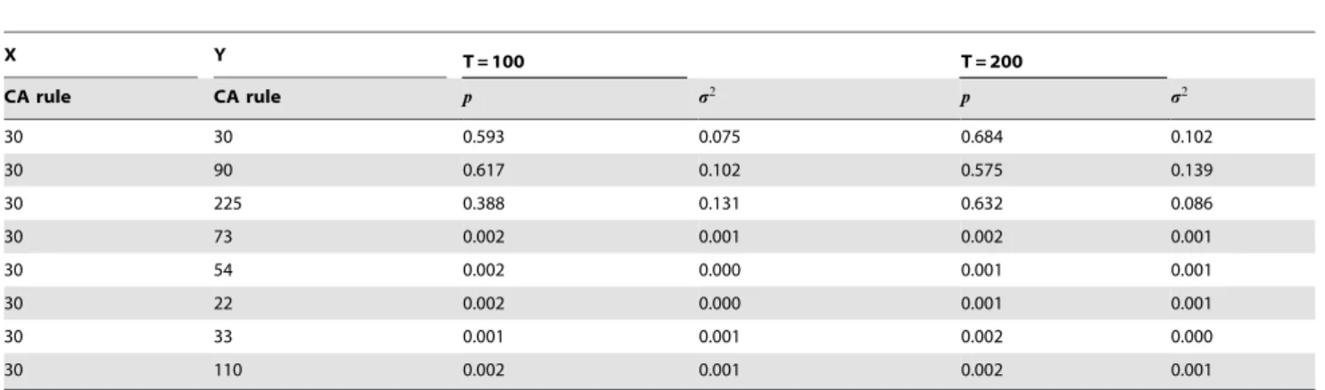
The first characteristic of the statistic complexity we study is the influence of the sizemof objects onCS. Table 1 shows the results for comparing patterns generated by different rules of one-dimensional cellular automata. Column one represents the reference process,X, and column two corresponds toY. The third and fifty column shows the averaged p-values obtained for cellular automata of lengthT~100
respectivelyT~200- column four and six provide the variances for the corresponding p-values. For the simulation results shown in Table 1 we generated spatiotemporal patterns for one-dimensional CA for N~50 (space) andT (time), an alphabet of sizek~2and ar~1
neighborhood with periodic boundary conditions. As burn-in time we usedttrans~1000time steps. Each of these spatiotemporal patternSij, withi[f1,. . .,Tgandj[f1,. . .,Ng, is transformed to its difference
Table 1.Results for one-dimensional CA (ttrans~1000,N~50,T~100(third and fourth column) andT~200(fifth and sixth
column)) averaged over10runs.
X Y T = 100 T = 200
CA rule CA rule p s2 p s2
30 30 0.593 0.075 0.684 0.102
30 90 0.617 0.102 0.575 0.139
30 225 0.388 0.131 0.632 0.086
30 73 0.002 0.001 0.002 0.001
30 54 0.002 0.000 0.001 0.001
30 22 0.002 0.000 0.001 0.001
30 33 0.001 0.001 0.002 0.000
30 110 0.002 0.001 0.002 0.001
pattern S?ððS2{S1ÞzðS3{S2Þz. . .zðST{ST{1ÞÞ (Here Si withi[f1,. . .,Tgcorresponds to a row vector of lengthN.) resulting in a string (object) of lengthm~NT to be applicable for the NCD. Here, the operatorzmeans concatenation of strings. See [29] for numerical details for the application of NCD. The results in Table 1 show that the p-values remain in the same order of magnitude if the size of an objectmis doubled meaning that the overall quantitative assessment of two processes X andY - based on sampled objects thereof - by the measureCSis invariant to extensions of the sizem. Next we demonstrate that thestatistic complexityis capable to differentiate between random and complex objects. For this reason we compare rule30, producing random patterns, with rule90,225, both random, and rule110, which is complex because it is capable of universal computation. From Table 1 one can see that the p-values correspond with our expectations giving high values forð30,90Þandð30,225Þand low values forð30,110Þ. In addition we compare rule30with rules
73,54and22, classified according to Wolfram as random, and obtain very low p-values, suggesting significant differences among those patterns. The crucial point here is that not all CA rules that produce chaotic patterns are indistinguishable from each other. In [33] the growth exponent of the roughness along other measures have been used to obtain several subclasses for CA rules leading to chaotic behavior. Comparing our results with their classification reveals that actually rule73,54and22are in different subclasses whereas rule30is classified together with rule90and225. Last, we compare rule30with a periodic pattern, rule 33, and obtain also in this case a clear distinction. In summary,CScan not only distinguish between simple and complex patterns but finds also meaningful substructures among chaotic patterns if rule30is used as reference process.
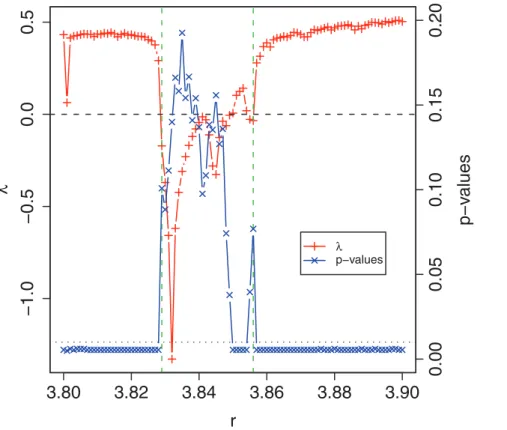
Next, we apply our measure to the logistic map and compare the results with the Lyapunov exponent (l). The results are summarized in Fig. 2. We calculate the time series for various
values ofr(x-axis) in the intervall½3:8, 3:9(rwas varied in step sizes of0:001and sample size wasn1~n2~6.).lassumes negative
values in½3:829, 3:849and½3:856, 3:856indicating a nonchaotic behavior of the logistic map for these values of r. The vertical dashed line separates positive from negative values. The p-values of thestatistic complexity(blue line, cross symbols) are obtained for each value ofrby averaging over 50 time series each of length
1000(After waiting a transient period of1000steps.). As reference process, X, we use a logistic map with rref~3:451, which corresponds to a periodic behavior. From Fig. 2 one can see that there are essentially two types of p-values, ones that are not zero and ones that are close to zero. For example, using a significance level of0:01 (dotted horizontal line) one obtains that significant values correspond to positive Lyapunov exponents and non-significant values to negative Lyapunov exponents. Again, we want to emphasize that the p-values do not provide a yes or no answer if the logistic map, for a givenrvalue, is chaotic or nonchaotic but the correct interpretation is that low p-values provide strong evidence against the null hypotheses whereas high p-values do not allow to reject the null hypotheses. Because we userref~3:451as reference - for which the logistic map shows periodic (nonchaotic) behavior - this is a similar though not identical question. The results for the logistic map allow a comparison with a well studied system. As demonstrated by our results shown in Fig. 2, for an appropriately chosen reference process, X rref
, there is a clear correspondence between thestatistic complexity and the Lyapunov exponent. This property is certainly desirable to hold because it may allows to connect to traditional contributions in the field beyond the logistic map. The possibility of such a connection, despite the seemingly different methods underlying the statistic complexityrespectively the Lyapunov exponent, can be attributed to the parametric form of our complexity measure allowing a
Figure 2. Lyapunov exponent (l- red line, plus symbol) and p-values (blue line, cross symbol) of the logistic map in dependence on
r.The dotted horizontal line corresponds to a significance level of0:01and the dashed line tol~0.
flexibility that is entirely missing in other measures. More importantly, this flexibility is not imposed into the measure but follows naturally from a consequent interpretation of complexity as a referential measure [12] implying imperatively the existence of a reference process X against which another process Y is
quantitativelycompared.
Discussion
The complexity measure introduced in this paper has several properties that are different to all other measures proposed so far. First, CS is a bivariate measure allowing to make comparative statements, instead of absolute ones. This may appear as a disadvantage first, however, as LO´ PEZ-RUIZet al. [12] point out, we inevitably compare patterns with each other to make a decision about their complexity (See also thecomparativediscussion on page 909 in [17] about the three patterns shown in Fig. 1.) [20]. Second, we do not make assumptions with respect to the size of patterns to which our measure can be applied, instead, principally, we allow patterns of any finite or infinite sizem. For example, measures like EMC orexcess entropyare based on block entropies of varying order n and the final measure is obtained in the limit for n against infinity. Strictly, such measures require an infinite amount of data. Third, due to the fact thatstatistic complexityallows the comparison of patterns of any size mwith finite sample sizes n1 and n2 the
result of the comparison may be erroneous. The KS test, underlyingCS, allows a quantification of such an error statistically. Because this error can be quantified in dependence onm,n1and n2, there is no need to assume limiting properties. At this point we
would like to re-emphasize that the termstatistic complexityhas been chosen to underline the involvement of atest statisticin our measure on which the complexity value is based. For this reason other complexity measures that have been named statistical complexity
[12,34,35] are not similar to our measure at all due to the fact that none of these measures uses a test statistic or a statistical test. Hence, they are actually not related to statistics (the field). An alternative name for these measures would beprobabilistic complexity, which would make this difference more obvious. The fourth point
relates to the empirical distribution functions. The reason for their introduction is, besides the fact that they allow a connection to the KS test, they allow the introduction of two ensembles, one for the processXand one for processesY. These ensembles compensate that the classic KOLMOGOROV complexity is not related to any ensemble but only to one string. Further, the ensembles induce a probabilistic interpretation of the deterministic NCD with respect to the underlying processes that generate the patterns. This is in accordance with [17] emphasizing the importance of complexity measures being probabilistic. Taken together, this allows a quantifiable approximation, in dependence onm, n1 and n2, of
the underlying processesXandYwith respect to the information they provide about their complexity, in form of the real observable patterns.
From an applied point of view, the direct connection ofstatistic complexitywith statistical inference allows a confirmatory analysis of the complexity of objects. Due to the fact that the uncertainty of a complexity comparison is inherently provided by our measure, it is applicable to (real) objects from a multitude of different application domains. In the future we are planing to investigate the complexity of biological pathways in the context of cancer and other complex diseases [37]. A further potential direction would be an analysis of differentgoodness-of-fittests. For example, it would be interesting to study a Crame´r-von Mises or an Anderson-Darling test, instead of a Kolmogorov-Smirnov test [36]. Other tests may have advan-tages in different application areas or specific experimental conditions, although, a Kolmogorov-Smirnov test was sufficient with respect to the applications studied in this paper.
Acknowledgments
For the statistical simulations R [38] has been used.
Author Contributions
Conceived and designed the experiments: FES. Performed the experi-ments: FES. Analyzed the data: FES. Contributed reagents/materials/ analysis tools: FES. Wrote the paper: FES.
References
1. Bar-Yam Y (1997) Dynamics of Complex Systems. Perseus Books. 2. Nicolis G, Prigogine I (1989) Exploring Complexity. Freeman.
3. Prokopenko M, Boschetti F, Ryan A (2009) An information-theoretic primer on complexity, self-organization, and emergence. Complexity 15: 11–28. 4. Schuster H (2002) Complex Adaptive Systems. Scator Verlag.
5. Wolfram S (1983) Statistical mechanics of cellular automata. Phys Rev E 55: 601–644.
6. Dehmer M (2008) A novel method for measuring the structural information content of networks. Cybernetics and Systems 39: 825–842.
7. Dehmer M, Barbarini N, Varmuza K, Graber A (2009) A large scale analysis of information-theoretic network complexity measures using chemical structures. PLoS ONE 4: e8057.
8. Watts D, Strogatz S (1998) Collective dynamics of ‘small-world’ networks. Nature 393: 440–442.
9. Kolmogorov AN (1965) Three approaches to the quantitative definition of ‘information’. Problems of Information Transmission 1: 1–7.
10. Li M, Vita´nyi P (1997) An Introduction to Kolmogorov Complexity and Its Applications Springer.
11. Solomonoff R (1960) A preliminary report on a general theory of inductive inference. Technical Report V-131, Zator Co., Cambridge, Ma.
12. Lo´pez-Ruiza R, Mancinib H, Calbet X (1995) A statistical measure of complexity. Physics Letters A 209: 321–326.
13. Badii R, Politi A (1997) Complexity: Hierarchical Structures and Scaling in Physics. Cambridge University Press, Cambridge.
14. Bennett C (1988) Logical depth and physical complexity. In: Herken R, ed. The Universal Turing Machine– a Half-Century Survey Oxford University Press. pp 227–257.
15. Crutchfield JP, Young K (1989) Inferring statistical complexity. Phys Rev Lett 63: 105–108.
16. Gell-Mann M, Lloyd S (1998) Information measures, effective complexity, and total information. Complexity 2: 44–52.
17. Grassberger P (1986) Toward a quantitative theory of self-generated complexity. Int J Theor Phys 25: 907–938.
18. Lloyd S, Pagels H (1988) Complexity as thermodynamic depth. Annals of Physics 188: 186–213.
19. Zurek W, ed (1990) Complexity, Entropy and the Physics of Information. Addison-Wesley, Redwood City.
20. Grassberger P (1989) Problems in quantifying self-generated complexity. Helvetica Physica Acta 62: 489–511.
21. Chaitin G (1966) On the length of programs for computing finite binary sequences. Journal of the ACM. pp 547–569.
22. Crutchfield J, Packard N (1983) Symbolic dynamics of noisy chaos. Physica D 7: 201–223.
23. Bialek W, Nemenman I, Tishby N (2001) Predictability, complexity, and learning. Neural Computation 13: 2409–2463.
24. Cilibrasi R, Vita´nyi P (2005) Clustering by compression. IEEE Transactions Information Theory 51: 1523–1545.
25. Casella G, Berger R (2002) Statistical Inference. Duxbury Press.
26. Mood A, Graybill F, Boes D (1974) Introduction to the Theory of Statistics McGrw-Hill.
27. Li M, Chen X, Li X, Ma B, Vita´nyi P (2004) The similarity metric. IEEE Transactions on Information Theory 50: 3250–3264.
28. Cebrian M, Alfonseca M, Ortega A (2005) Common pitfalls using the normalized compression distance: What to watch out for in a compressor. Communications in Information and Systems 5: 367–384.
29. Emmert-Streib F (2010) Exploratory analysis of spatiotemporal patterns of cellular automata by clustering compressibility. Physical Review E 81: 026103.
30. Conover W (1999) Practical Nonparametric Statistics. John Wiley & Sons, New York.
32. Milbrodt H, Strasser H (1990) On the asymptotic power of the two-sided kolmogorov-smirnov test. Journal of Statistical Planning and Inference 26: 1–23. 33. Mattos T, Moreira J (2004) Universality Classes of Chaotic Cellular Automata.
Brazilian Journal of Physics 34: 448–451.
34. Crutchfield J, Feldman D (1997) Statistical complexity of simple one-dimensional spin systems. Phys Rev E 55: R1239.
35. Feldman D, Crutchfield J (1998) Measures of statistical complexity: Why? Physics Letters A 238: 244–252.
36. Lehman E (2005) Testing Statistical Hypotheses. Springer.
37. Emmert-Streib F (2007) The chronic fatigue syndrome: A comparative pathway analysis. Journal of Computational Biology 14: 961–972.