Submitted28 July 2016 Accepted 4 October 2016 Published14 November 2016
Corresponding author
Gaëtan Benoit, [email protected]
Academic editor C. Titus Brown
Additional Information and Declarations can be found on page 21
DOI10.7717/peerj-cs.94
Copyright 2016 Benoit et al.
Distributed under
Creative Commons CC-BY 4.0
OPEN ACCESS
Multiple comparative metagenomics
using multiset
k
-mer counting
Gaëtan Benoit1, Pierre Peterlongo1, Mahendra Mariadassou2, Erwan Drezen1,3,
Sophie Schbath2, Dominique Lavenier1and Claire Lemaitre1
1Inria Rennes Bretagne Atlantique - IRISA, GenScale team, Rennes, France 2MaIAGE, INRA, Université Paris-Saclay, Jouy-en-Josas, France
3CHU Pontchaillou, Rennes, France
ABSTRACT
Background. Large scale metagenomic projects aim to extract biodiversity knowledge
between different environmental conditions. Current methods for comparing microbial communities face important limitations. Those based on taxonomical or functional assignation rely on a small subset of the sequences that can be associated to known organisms. On the other hand, de novo methods, that compare the whole sets of sequences, either do not scale up on ambitious metagenomic projects or do not provide precise and exhaustive results.
Methods. These limitations motivated the development of a newde novometagenomic
comparative method, called Simka. This method computes a large collection of standard ecological distances by replacing species counts by k-mer counts. Simka scales-up today’s metagenomic projects thanks to a new parallel k-mer counting strategy on multiple datasets.
Results. Experiments on public Human Microbiome Project datasets demonstrate that
Simka captures the essential underlying biological structure. Simka was able to compute in a few hours both qualitative and quantitative ecological distances on hundreds of metagenomic samples (690 samples, 32 billions of reads). We also demonstrate that analyzing metagenomes at thek-mer level is highly correlated with extremely precisede novocomparison techniques which rely on all-versus-all sequences alignment strategy or which are based on taxonomic profiling.
SubjectsBioinformatics, Computational Biology
Keywords Comparative metagenomics,k-mer,k-mer counting, Metagenomic, Large scale, Ecological distance, Ngs
INTRODUCTION
It is estimated that only a fraction of 10−24–10−22 of the total DNA on earth has
been sequenced (Anonymous, 2011). In large scale metagenomics studies such asTara
composition. Such compositions may be approximated by sequencing marker genes, such as the rRNA 16S in bacterial communities (Liles et al., 2003), and clustering the sequences into Operational Taxonomic Units (OTU) or working species. However, marker genes surveys suffer from amplification and primer bias (Cai et al., 2013) and therefore may not capture the whole microbial diversity of a sample. Furthermore, even within the captured diversity, the marker may not be informative enough to discriminate between sub-species or even species strains (Piganeau et al., 2011). Finally, this approach is impractical for whole metagenomic sets for at least two reasons: clustering reads into putative species is computationally costly and leaves out a large fraction of the reads (Nielsen et al., 2014).
In this context, it is more practical to ditch species composition altogether and compare microbial communities using directly the sequence content of metagenomic read sets. This has first been performed by using Blast (Altschul et al., 1990) for comparing read content (Yooseph et al., 2007). This approach was successful but cannot scale up to large studies made up of dozens or hundreds of large read sets, such as those generated from Illumina sequencers.
In 2012, the Compareads method (Maillet et al., 2012) was proposed. The method compares the whole sequence content of two read sets. It introduced a rough approximation of read similarity based on the number of shared words of lengthk(k-mer, withktypically around 30) and used it for providing so defined similar reads between read sets. The number of similar reads was then used for computing a Jaccard distance between pairs of read sets. Commet (Maillet et al., 2014) is an extended version of Compareads. It better handles the comparison of large read sets and provides a read sub-set representation that facilitates result analyses and reduces the disk footprint.Seth et al. (2014)used the notion of sharedk-mers between samples for estimating dataset similarities. This is a slightly different problem as this was used for retrieving from an indexed database, samples similar to a query sample. More recently, two additional methods were developed to represent a metagenome by a feature vector that is then used to compute pairwise similarity matrices between multiple samples. For both methods, features are based on thek-mer composition of samples, but with a feature representing more than onek-mer and using only a subset ofk-mers to reduce the dimension (Ulyantsev et al., 2016;Ondov et al., 2016). However, the approaches fork-mer grouping and sub-sampling are radically different. In MetaFast (Ulyantsev et al., 2016), the subset ofk-mers is obtained by post-processingde novoassemblies performed for each metagenome. A feature represents then a set of k-mers belonging to a same assembly graph ‘‘component.’’ The relative abundance of such component in each sample is then used to compute the Bray–Curtis dissimilarity measure. In Mash (Ondov et al., 2016), a sub-sampling of thek-mers is performed using the MinHash (Broder, 1997) approach (keeping by default 1,000k-mers per sample). The method outputs then a Jaccard index of the presence-absence of suchk-mers in two samples.
All these reference-free methods share the use ofk-mers as the fundamental unit used for comparing samples. Actually,k-mers are a natural unit for comparing communities: (1) sufficiently long k-mers are usually specific of a genome (Fofanov et al., 2004); (2)
same bacterial species) without need for a classification of those organisms (Teeling et al., 2004).Dubinkina et al. (2016)conducted an extensive comparison betweenk-mer-based distances and taxonomic ones (i.e., based on taxonomic assignation against a reference database) for several large scale metagenomic projects. They demonstrate thatk-mer-based distances are well correlated to taxonomic ones, and are therefore accurate enough to recover known biological structure, but also to uncover previously unknown biological features that were missed by reference-based approaches due to incompleteness of reference databases. Importantly, the greaterk, the more correlated these taxonomic andk -mer-based distances seem to be. However, the study is limited to values ofk lower than 11 for computational reasons and the correlation for large values ofkstill needs to be evaluated.
Even if Commet and MetaFast approaches were designed to scale-up to large metagenomic read sets, their use on data generated by large scale projects is turning into a bottleneck in terms of time and/or memory requirements. By contrast, Mash outperforms by far all other methods in terms of computational resource usage. However, this frugality comes at the expense of result quality and precision: the output distances and Jaccard indexes do not take into account relative abundance information and are not computed exactly due tok-mer sub-sampling.
In this paper, we present Simka. Simka comparesN metagenomic datasets based on theirk-mers counts. It computes a large collection of distances classically used in ecology to compare communities. Computation is performed by replacing species counts byk-mer counts, for a large range of kmer sizes, including large ones (up to 30). Simka is, to our knowledge, the first method able to rapidly compute a full range of distances enabling the comparison of any number of datasets. This is performed by processing data on-the-fly (i.e., without storage of large temporary results). With the exception of Mash that is, thanks to sub-sampling, approximately two to five time faster, Simka outperforms state-of-the-art read comparison methods in terms of computational needs. For instance, Simka ran on 690 samples from the Human Microbiome Project (HMP) (Human Microbiome Project Consortium, 2012a) (totalling 32 billion reads) in less than 10 h and using no more than 70 GB RAM.
The contributions of this manuscript are three-fold. First we propose a new method for efficiently countingk-mers from a large number of metagenomic samples. The usefulness of such counting is not limited to comparative metagenomics and may have applications in many other fields. Second, we show how to derive a large number of ecological distances fromk-mer counts. And third, we show on real datasets thatk-mer-based distances are highly correlated to taxonomic distances: they therefore capture the same underlying structure and lead to the same conclusions.
MATERIALS AND METHODS
Overview
GivenN metagenomic datasets, denoted as S1,S2,Si,...,SN, the objective is to provide aN×N distance matrixDwhereDi,j represents an ecological distance between datasets
Si andSj. Such possible distances are listed inTable 1. The computation of the distance matrix can be theoretically decomposed into two distinct steps:
1. k-mer count. Each dataset is represented as a set of discriminant features, in our case,
k-mer counts. More precisely, ak-mer count matrixKC of sizeW×N is computed.
W is the number of distinctk-mer among all the datasets.KCi,j represents the number of times ak-meriis present in the datasetSj.
2. distance computation. Based on the k-mer count information, the distance matrix
Dis computed. Actually, many ecological distances (cfTable 1) can be derived from matrixKCwhen replacing species counts byk-mer counts.
Actually, Simka does not require to have the fullKC matrix to start the distance com-putation. However, for sake of simplicity, we will first consider this matrix to be available.
Thek-mer count step splits all the reads of the datasets intok-mers and performs a global count. This can be done by counting individually k-mers in each dataset, then merging the overallk-mer counts. The output is the matrixKC (of sizeW×N). Efficient algorithms, such as KMC2 (Deorowicz et al., 2015), have recently been developed to count all the occurrences of distinctk-mers in a read dataset, allowing the computation to be executed in a reasonable amount of time and memory even on very large datasets. However, the main drawback of this approach is the huge main memory space it requires which is computed as follow:MemKC=Ws∗(8+4N) bytes, withWsthe number of distinctk-mers,
N the number of samples, and 8 and 4 the number of bytes required to store respectively 31-mers and ak-mer count. For example, experiments on the HMP (Human Microbiome Project Consortium, 2012a) datasets (690 datasets containing on average 45 millions of reads each) would require a storage space of 260TBfor the matrixKC.
However, a careful look at the definition of ecological distances (Table 1) shows that, up to some final transformation, they are all additive over the k-mers. Independent contributions to the distance can thus be computed in parallel from disjoint sets of
k-mers and aggregated later on to construct the final distance matrix. Furthermore, each independent contribution can itself be constructed in an iterative way by receiving lines of theKCmatrix, called abundance vectors, one at a time. The abundance vector of a specific
k-mer simply consists of itsN counts in theN datasets.
Table 1 Definition of some classical ecological distances computed by Simka.All quantitative distances can be expressed in terms ofCS,f =
f(x,y,X,Y) andg=g(x), using the notations ofEq. (2), and computed in one pass. Qualitative ecological distances (resp. AB-variants of qualita-tive distances) can also be computed in a single pass over the data by computing firsta,bandc(resp.UandV). See main text for the definition of a,b,c,UandV.
Name Definition CSi f(x,y,X,Y) g(x)
Quantitative distances
Chord r
2−2P
w
NSi(w)NSj(w) CSiCSj
pP
wNSi(w)2
xy XY
√
2−2x
Hellinger r
2−2P
w
√N
Si(w)NSj(w)
√C
SiCSj
P
wNSi(w)
√xy √
XY
√
2−2x
Whittaker 1
2
P
w
NSi(w)CSj−NSj(w)CSi CSiCSj
P
wNSi(w) |
xY−yX|
XY
x 2
Bray–Curtis 1−2P
w
min(NSi(w),NSj(w)) CSi+CSj
P
wNSi(w)
min(x,y)
X+Y 1−2x
Kulczynski 1−1
2
P
w
(CSi+CSj)min(NSi(w),NSj(w)) CSiCSj
P
wNSi(w)
(X+Y)min(x,y)
XY 1−
x 2
Jensen–Shannon v
u u u u u u u t
1 2
X
w
"
NSi(w)
CSi
log 2CSjNSi(w) CSjNSi(w)+CSiNSj(w)
+
NSj(w)
CSj
log 2CSiNSj(w) CSjNSi(w)+CSiNSj(w)
#
P
wNSi(w) XxlogxY2xY+yX+
y Ylog
2yX xY+yX
px 2
Canberra 1
a+b+c
P
w
NSi(w)−NSj(w) NSi(w)+NSj(w)
−
x−y x+y
1 a+b+cx
Qualitative distances
Chord/Hellinger r
21−√ a (a+b)(a+c)
– – –
Whittaker 1
2 b a+b+
c a+c+
aa
+b− a a+c
– – –
Bray–Curtis/Sorensen b+c
2a+b+c – – –
Kulczynski 1−1
2 a a+b+
a a+c
– – –
Ochiai 1−√ a
(a+b)(a+c) – – –
Jaccard b+c
a+b+c – – –
Abundance-based (AB) variants of qualitative distances
AB-Jaccard 1− UV
U+V−UV – – –
AB-Ochiai 1−√UV – – –
AB-Sorensen 1− 2UV
S1 S2 … SN
S1 0 0.2 … 0.1
S2 0.2 0 … 0.4
… … … … …
SN 0.1 0.4 … 0 Read
set S1
Read set S2
Read set SN
Accumulate contribu:ons and
compute final distance matrix
…
Generate abundance
vectors
Update par:al contribu:on to the distance
Update par:al contribu:on to the distance
Update par:al contribu:on to the distance
Update par:al contribu:on to the distance
…
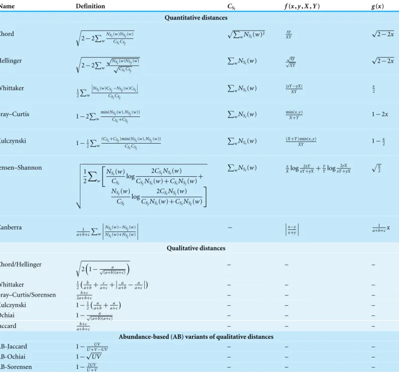
Figure 1 Simka strategy.The first step takes as inputNdatasets and generates multiple streams of abun-dance vector from disjoint sets ofk-mers. The abundance vector of ak-mer consists of itsNcounts in the Ndatasets. These abundance vectors are taken as input by the second step to iteratively update indepen-dent contributions to the ecological distance in parallel. Once an abundance vector has been processed, there is no need to keep it on record. The final step aggregates each contribution and computes the final distance matrix.
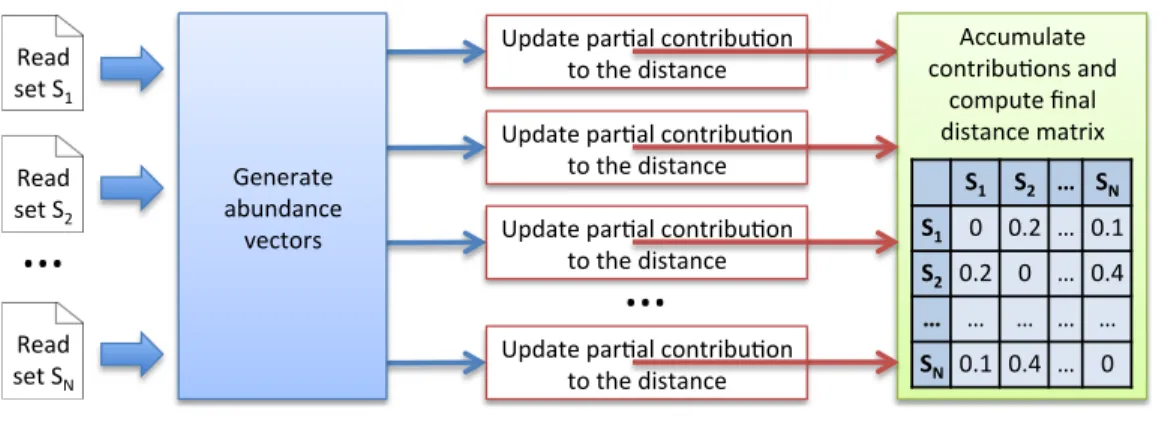
Multisetk-mer Counting
Starting from N datasets of reads, the aim is to generate abundance vectors that will feed the ecological distance computation step. This task is divided into two phases:
1. Sorting Count, 2. Merging Count.
Sorting Count. Eachk-mer of a dataset is extracted and its canonical representation is stored (the canonical representation of ak-mer is the smallest lexicographic value between thek-mer and its reverse complement). Canonicalk-mers are then sorted in lexicographical order. Distinctk-mers can thus be identified and their number of occurrences computed.
As the number of distinct k-mers is generally huge, the sorting step is divided into two sub-tasks and proceeds as follows: thek-mers are first separated intoP partitions, each stored on disk. After this preliminary task, each partition is sorted and counted independently, and stored again on disk. Conceptually, at the end of the sorting count process, we dispose ofN×Psorted partitions. As the same distribution function is applied to all datasets, a partitionPicontains a specific subset ofk-mers common to all datasets. Figure 2Aillustrates the Sorting Count phase.
The Sorting Count phase has a high parallelism potential. A first parallelism level is given by the independent counts of each dataset.N processes can thus be run in parallel, each one dealing with a specific dataset. A second level is given by the fine grained parallelism implemented in software such as DSK (Rizk, Lavenier & Chikhi, 2013) or KMC2 (Deorowicz et al., 2015) that intensively exploit today multicore processor capabilities. Thus, the overall Sorting Count process is especially suited for grid infrastructures made of hundred of nodes, and where each node implements 8 or 16-core systems.
Read set S1
Read Set S2
Read set SN
CAT 1
ATC 4
AAG 2 TTA 4
AAG 8 GGC 1
GGC 9 TTA 1 ACG 4
TTG 2
ATC 8
ACG 1
ATC 2 CGG 4
S1 S2 SN
ACG 0 4 1
P
p
ar
3
3
o
n
s
CAG 7 CAG 3 CAG 1
GAC 6 (A) Sort and Count k‐mers
(B) Merge k‐mer counts
S1 S2 SN
CAT 1 0 0
S1 S2 SN
TTG 0 2 0
S1 S2 SN
ATC 4 8 2
S1 S2 SN
CGG 0 0 4
S1 S2 SN
AAG 2 8 0
S1 S2 SN
GGC 0 1 9
S1 S2 SN
TTA 4 0 1
S1 S2 SN
CAG 7 3 1
S1 S2 SN
GAC 0 0 6
Streams of abundance vectors
Figure 2 Multisetk-mer Counting strategy withk=3.(A) The sorting counting process, represented
by a blue arrow, counts datasets independently. Each process outputs a column ofPpartitions (red squares) containing sortedk-mer counts. (B) The merging count process, represented by a green arrow, merges a row ofNpartitions. It outputs abundance vectors, represented in green, to feed the ecological distance computation process.
Merging Count. Here, the data partitioning introduced in the previous step is advantageously used to generate abundance vectors. TheN files associated to a partition
Pi, are taken as input of a merging process. These files containk-mer counts sorted in lexicographical order. A Merge-Sort algorithm can thus be efficiently applied to directly generate abundance vectors.
In that scheme,P processes can be run independently, resulting in the generation ofP
abundance vectors in parallel, allowing to compute simultaneouslyPcontributions of the ecological distance. Note that the abundance vectors do not need to be stored. They are only used as input streams for the next step.Figure 2Billustrates the Merging Count phase.
k-mer abundance filter. Distinctk-mers with very low abundance usually come from sequencing errors. As a matter of fact, a single sequencing error creates up tok erroneous distinctk-mers. Filtering out thesek-mers speeds-up the Simka process, as it greatly reduces the overall number of distinctk-mers, but may also impact the content of the distance matrix. This point is evaluated and discussed in the result section.
Ecological distance computation
Simka computes a collection of distances for all pairs of datasets. As detailed in the previous section, abundance vectors are used as input data. For the sake of simplicity, we first explain the computations of the Bray–Curtis distance. All other distances, presented later on, can be computed in the same way, with only small adaptations.
Computing the Bray–Curtis distance. The Bray–Curtis distance is given by the following equation:
BrayCurtisAb(Si,Sj)=1−2 P
w∈Si∩Sjmin(NSi(w),NSj(w))
P
w∈SiNSi(w)+
P
w∈SjNSj(w)
(1)
wherewis ak-mer andNSi(w) is the abundance ofwin the datasetSi. We consider here
thatw∈Si∩SjifNSi(w)>0 andNSj(w)>0.
The equation involves marginal (or dataset specific) terms (i.e.,P
w∈SiNSi(w) is the total
amount ofk-mers in dataset Si) acting as normalizing constants and crossed terms that capture the (dis)similarity between datasets (i.e.,P
w∈Si∩Sjmin(NSi(w),NSj(w)) is the total
amount ofk-mers in the intersection of the datasetsSiandSj). Marginal and crossed terms are then combined to compute the final distance.
Algorithm 1 shows that it is straightforward to compute the distance matrix betweenN
datasets from the abundance vectors. Inputs of this algorithm are provided by the Multiple
k-mer Counting algorithm (MKC). These are theP streams of abundance vectors and the marginal terms of the distance, i.e., the number ofk-mers in each dataset, determined during the first step of the MKC which counts thek-mers.
A matrix, denoted M∩, of dimensionN×N is initialized (step 1) to record the final value of the crossed terms of each pair of datasets.P independent processes are run (step 2) to computeP partial crossed term matrices, denotedM∩part (step 3), in parallel. Each process iterates over its abundance vector stream (step 4). For each abundance vector, we loop over each possible pair of datasets (steps 5–6). The matrixM∩part is updated (step 8) if thek-mer is shared, meaning that it has positive abundance in both datasetsSi andSj (step 7). Since a distance matrix is symmetric with null diagonal, we limit the computation to the upper triangular part of the matrixM∩part. The current abundance vector is then released. Each process writes its matrixM∩part on the disk when its stream is done (step 9).
When all streams are done, the algorithm reads each writtenM∩part and accumulates it toM∩(step 10–11). The last loop (steps 13–16) computes the Bray–Curtis distance for each pair of datasets and fills the distance matrix reported by Simka.
The amount of abundance vectors streamed by the MKC is equal toWs, which is also the total amount of distinct solidk-mers in theN datasets. This algorithm has thus a time complexity ofO(Ws×N2).
Algorithm 1:Compute the Bray-Curtis distance (Eq. (1)) betweenN datasets
Input:
-Vs: vector of sizePrepresenting the abundance vector streams -V∪: vector of sizeN containing the number ofk-mers in each dataset
Output:a distance matrixDist
1 M∩←empty square matrix of sizeN // number ofk-mers in each dataset
intersec-tion
2 In parallel: foreachabundance vector stream SinVsdo
3 M∩part ←empty squared matrix of sizeN // part ofM∩
4 foreachabundance vector vinSdo
5 fori←0toN−1do
6 forj←i+1toN−1do
7 ifv[i]>0and v[j]>0then
8 M∩part[i,j] ←M∩part[i,j] +min(v[i],v[j])
9 WriteM∩part to disk
10 foreacheachwritten matrix M∩part do
11 M∩←M∩+M∩part
12 Dist ←empty squared matrix of sizeN// final distance matrix
13 fori←0toN−1do
14 forj←i+1toN−1do
15 Dist[i,j] =1−2∗M∩[i,j]/(V∪[i] +V∪[j])
16 Dist[j,i] =1−2∗M∩[i,j]/(V∪[i] +V∪[j])
17 returnDist
based on proper abundance data (hereafter called quantitative). Qualitative distances are more sensitive to factors that affect presence-absence of organisms (such as pH, salinity, depth, humidity, absence of light, etc.) and therefore useful to study bioregions. Quantitative distances focus on factors that affect relative changes (seasonal changes, nutrient availability, concentration of oxygen, depth, diet, disease, etc.) and are therefore useful to monitor communities over time or along an environmental gradient. Note that some factors, such as pH, are likely to affect both presence-absence (for large changes in pH) and relative abundances (for small changes in pH). Algorithmically, most ecological distances, including most of those mentioned in Legendre & De Cáceres (2013), can be expressed for two datasetsSiandSj as:
Distance(Si,Sj)=g
X
w∈Si∪Sj
f NSi(w),NSj(w),CSi,CSj
(2)
whereg andf are simple functions, andCSi is a marginal (i.e., dataset-specific) term of
of k-mers in Si. By contrast, the value off corresponds to crossed terms and requires knowledge of bothNSi(w) andNSj(w) (and potentiallyCSi andCSj as well). For instance,
for the abundance-based Bray–Curtis distance of Eq. (1), we haveCSi=
P
w∈SiNSi(w), g(x)=1−2xandf(x,y,X,Y)=min(x,y)/(X+Y). Those distances can be computed in a single pass over the data using a slightly modified variant of Algorithm 1. The marginal termsCSi are computed during the first step of the MKC which counts thek-mers of each
dataset. The crossed terms involvingf are computed and summed in steps 7–8 (but exact instructions depend on the nature off). Finally, the actual distances are computed in steps 15–16 and depend on bothf andg.
Qualitative distances form a special case of ecological distances: they can all be expressed in terms of quantitiesa,bandcwhereais the number of distinctk-mers shared between datasetsSi andSj,bis the number of distinctk-mers specific to datasetSi andc is the number of distinctk-mers specific to datasetSj. Those distances easily fit in the previous framework asa=P
w∈Si∩Sj1{NSi(w)NSj(w)>0},CSi=
P
w∈Si1{NSi(w)>0}=a+band similarly CSj=a+c. Therefore, ais a crossed term and bandc can be deduced fromaand the
marginal terms.
In the same vein,Chao et al. (2006)introduced variations of presence-absence distances incorporating abundance information to account for unobserved species. The main idea is to replace ‘‘hard’’ quantities such asa/(a+b), the fraction of distinctk-mers fromSishared withSj, by probabilistic ‘‘soft’’ ones: here the probabilityU∈ [0,1]that ak-mer fromSiis also found inSj. Similarly, the ‘‘hard’’ fractiona/(a+c) of distinctk-mers fromSjshared withSiis replaced by the ‘‘soft’’ probabilityVthat ak-mer fromSjis also found inSi.Uand
V play the same role asa,bandcdo in qualitative distances and are sufficient to compute the variants named AB-Jaccard, AB-Ochiai and AB-Sorensen. However and unlike the quantitiesa,b c, which can be observed from the data,UandV are not known in practice and must be estimated from the data.Chao et al. (2006)proposed several estimates forU
andV. The most elaborate ones attempt to correct for differences in sampling depths and unobserved species by considering the completek-mer counts vector of a sample. Those estimates are unfortunately untractable in our case as we stream only a fewk-mer counts at a time. Instead we resort to the simplest estimates presented inChao et al. (2006), which lend themselves well to the additive and distributed nature of Simka:U=YSiSj/CSi and V=YSjSi/CSj whereYSiSj=
P
w∈Si∩SjNSi(w)1{NSj(w)>0}andCSi=
P
w∈SiNSi(w). Note that YSiSj corresponds to crossed terms and is asymmetric, i.e.,YSiSj 6=YSjSi. Intuitively,U is
the fraction ofk-mers (not distinct anymore) fromSialso found inSjand therefore gives more weights to abundantk-mers that its qualitative counterparta/(a+b).
Table 1 gives the definitions of the collection of distances computed by Simka while replacing species counts byk-mer counts. These are qualitative, quantitative and abundance-based variants of qualitative ecological distances. The table also provides their expression in terms ofCi,f andg, adopting the notations ofEq. (2).
Finally, note that the additive nature of the computed distances over k-mers is instrumental in achieving a linear time complexity (inWs, the amount of distinct solid
species (Pavoine et al., 2011), or edit distances betweenk-mers as those complex distances require all versus allk-mer comparisons.
Implementation
Simka is based on the GATB library (Drezen et al., 2014), a C++ library optimized to handle very large sets ofk-mers. It includes a powerful implementation of the sorting count algorithm with the latest improvements in terms ofk-mer counting introduced by Deorowicz et al. (2015).
Simka is usable on standard computers and has also been entirely parallelized for grid or cloud systems. It automatically splits the process into jobs according to the available number of nodes and cores. These jobs are sent to the job scheduling system, while the overall synchronization is performed at the data level.
Simka is an open source software, distributed under GNU affero GPL License, available for download athttps://gatb.inria.fr/software/simka/.
RESULTS
First, Simka performances are evaluated in terms of computation time, memory footprint and disk usage and compared to those of other state of the art methods. Then, the Simka distances are evaluated with respect to de novoand reference-based distances and with respect to known biological results.
We conduct our numerical experiments on data from the Human Microbiome Project (HMP) (Human Microbiome Project Consortium, 2012a) which is currently one of the largest publicly available metagenomic datasets: 690 samples gathered from different human body sites (http://www.hmpdacc.org/HMASM/). The whole dataset contains 2*16 billions of Illumina paired reads distributed non uniformly across the 690 samples. One advantage of this dataset is that it has been extensively studied, in particular the microbial communities are relatively well represented in reference databases (Human Microbiome Project Consortium, 2012a; Human Microbiome Project Consortium, 2012b) (seehttp://hmpdacc.org/pubs/publications.php for a complete list).Article S1 details precisely how the datasets used for each experiment were built.
Performance evaluation
0 25 50 75 100
2 5 10 20 40
Samples
CPU time (min)
Simka
Complex distances
Simple distances
MKC−Merge
MKC−Count
A
● ● ● ● ●
0 100 200 300 400 500
2 5 10 20 40
Samples
CPU time (min)
● Simka
Commet
Metafast
Mash
B
● ● ● ● ●
0 5 10 15 20 25
2 5 10 20 40
Samples
Memor
y (GB)
● Simka
Commet
Metafast
Mash
C
● ● ●
●
●
0 5 10 15
2 5 10 20 40
Samples
Disk (GB)
● Simka
Commet
Metafast
Mash
D
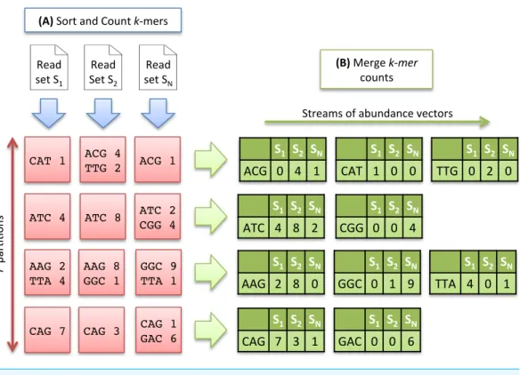
Figure 3 Simka performances with respect to the numberNof input samples. Each dataset is com-posed of two million reads. All tools were run on a machine equipped with a 2.50 GHz Intel E5-2640 CPU with 20 cores, 264 GB of memory. (A) and (B) CPU time with respect toN. For (A), colors correspond to different main Simka steps. (C) Memory footprint with respect toN. (D) Disk usage with respect toN. Parameters and command lines used for each tool are detailed inTable S1.
theoretical worst case quadratic time complexity relatively toN (the number of samples). The difference of execution time comes then from the amount of operations required, in practice, to calculate the crossed terms of the distances. For a given abundance vector, the simple distances only need to be updated for each pair (Si,Sj) such thatNSi>0 andNSj>0
whereas complex distances need to be updated for each pair such thatNSi>0 orNSj>0,
entailing a lot more update operations. It is noteworthy that among all distances listed inTable 1, all distances are simple, except the Whittaker, Jensen–Shannon and Canberra distances.
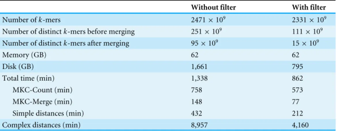
Table 2 Simka performances andk-mer statistics of the whole HMP project (690 samples).Simka was run on a machine equipped with a 2.50 GHz Intel E5-2640 CPU with 20 cores, 264 GB of memory, with k=31. Numbers of distinctk-mers are computed before and after the MKC-Merge algorithm: thebefore mergingnumber is obtained by summing over all samples the distinctk-mers computed for each sample independently, whereas in theafter mergingnumber,k-mers shared by several samples are counted only once. Line ‘‘Total time’’ does not include complex distances whose computation is optional.
HMP-690 samples-3727 GB-2×16 billion paired reads
Without filter With filter
Number ofk-mers 2471×109 2331×109
Number of distinctk-mers before merging 251×109 111×109
Number of distinctk-mers after merging 95×109 15
×109
Memory (GB) 62 62
Disk (GB) 1,661 795
Total time (min) 1,338 862
MKC-Count (min) 758 573
MKC-Merge (min) 148 77
Simple distances (min) 432 212
Complex distances (min) 8,957 4,160
compute only one such simple distance. TheFigs. 3B–3Dshows respectively the CPU time, the memory footprint and the disk usage of each tool with respect to an increasing number of samples N. Mash has definitely the best scalability but limitations of its computed distance are shown in the next section. Commet is the only one to show a quadratic time behaviour withN. ForN=40, Simka is 6 times faster than Metafast and 22 times faster than Commet. All tools, except Metafast, have a constant maximal memory footprint with respect toN. For metafast, we could not use its max memory usage option since it often created ‘‘out of memory’’ errors. The disk usage of the four tools increases linearly withN. The linear coefficient is greater for Simka and MetaFast, but it remains reasonable in the case of Simka, as it is close to half of the input data size, which was 11 GB forN=40.
In summary, Simka and Mash seems to be the only tools able to deal with very large metagenomics datasets, such as the full HMP project.
These results were obtained with default parameters, namely filtering outk-mers seen only once. On this dataset, this filter removes only 5 % of the data: solidk-mers (k-mers seen at least twice) account for 95% of all base pairs of the whole dataset (seeTable 2). But interestingly, when speaking in terms of distinctk-mers, solid distinctk-mers represent less than half of all distinct k-mers before merging across all samples and only 15% after merging. Consequently, Simka performances are greatly improved, both in terms of computation time and disk usage when considering only solidk-mers. Notably, this does not degrade distance quality, at least for the HMP dataset, as shown in the next section. Additional tests on the impact ofkon the performances show that the disk usage increases sub-linearly withk whereas the computation time and the memory usage stay constant (seeFig. S1).
Evaluation of the distances
We evaluate the quality of the distances computed by Simka answering two questions. First, are they similar to distances between read sets computed using other approaches? Second, do they recover the known biological structure of HMP samples? For the first evaluation, two types of other approaches are considered, eitherde novoones (similar to Simka but based on read comparisons), or taxonomic distances, e.g. approaches based on a reference database.
Correlation with read-based approaches. In this section, we focus on comparing Simka
k-mer-based distance to two read-based approaches: Commet (Maillet et al., 2014) and an alignment-based method using BLAT (Kent, 2002). Both these read-based approaches define and use a readsimilarity notion. They derive the percentage of reads from one sample similar to at least one read from the other sample as a quantitative similarity measure between samples. Commet considers that two reads are similar if they share at least t non-overlappingk-mers (heret=2,k=33). For BLAT alignments, similarity was defined based on several identity thresholds: two reads were considered similar if their alignment spanned at least 70 nucleotides and had a percentage of identity higher than 92%, 95% or 98%. For ease of comparison, Simka distance was transformed to a similarity measure, such as the percentage of shared kmers (see Article S1for details of transformation).
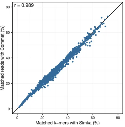
Looking at the correlation with Commet is interesting because this tool uses a heuristic based on sharedk-mers but its final distance is expressed in terms of read counts. As shown inFig. 4, on a dataset of 50 samples from the HMP project, Simka and Commet similarity measures are extremely well correlated (Spearman correlation coefficientr=0.989).
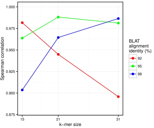
Similarly, clear correlations (r>0.89) are also observed between the percentage of matched k-mers and the percentage of similar reads as defined by BLAT alignments (Fig. 5). Interestingly, the correlation depends on thek-mer size and the identity threshold used for BLAT: largerk-mer sizes correlate better with higher identity thresholds andvice versa. The highest correlation is 0.987, obtained for Simka withk=21 compared to BLAT results with 95% identity.
● ● ● ● ● ● ● ● ● ● ● ● ● ● ● ● ● ● ● ● ● ● ● ● ● ● ● ● ● ●● ● ● ● ● ● ● ● ● ● ● ● ● ● ● ● ● ● ● ● ● ● ● ● ● ● ● ● ● ● ● ● ●●● ●● ● ● ● ● ● ● ● ● ●● ● ● ● ● ● ● ● ● ● ● ● ● ● ● ● ● ● ● ● ● ● ● ● ● ● ● ● ● ● ● ● ● ● ● ● ● ● ● ● ● ● ● ● ● ● ●● ● ● ● ● ● ● ● ● ● ● ● ● ●● ● ● ● ● ● ● ● ● ● ● ● ● ● ● ● ● ● ● ● ● ● ● ● ● ● ●● ● ● ● ● ● ● ● ● ● ● ● ● ● ● ● ● ● ● ● ● ● ● ● ● ● ● ● ● ● ● ● ● ● ● ● ● ● ● ● ● ● ● ● ● ● ● ● ● ● ● ● ● ● ● ● ● ● ● ●● ● ● ● ● ● ● ● ● ● ● ● ● ● ● ● ● ● ● ● ● ● ● ● ● ● ● ● ● ● ● ● ● ● ● ● ● ● ● ● ● ● ● ● ● ● ● ● ● ● ● ● ● ● ● ● ● ● ● ● ● ● ● ● ● ● ● ● ● ● ● ● ● ● ● ● ● ● ● ● ● ● ● ● ● ● ● ● ● ● ● ● ● ● ● ● ● ● ● ● ● ● ● ● ● ● ● ● ● ● ● ● ● ● ● ● ● ● ● ● ● ● ● ● ● ● ● ● ● ● ● ● ● ● ● ● ● ● ● ● ● ● ● ● ● ● ● ● ● ● ●● ● ● ● ● ● ● ● ● ● ● ● ● ● ● ● ● ●● ● ● ●● ● ● ● ● ● ● ● ● ● ● ● ● ● ● ● ● ● ● ● ● ● ●● ● ● ● ● ● ● ● ● ● ● ● ● ● ● ● ● ● ● ● ● ● ● ● ● ● ● ● ● ● ● ● ● ● ● ● ● ● ● ● ● ● ● ● ● ● ● ● ● ● ● ● ● ● ● ● ● ● ● ● ● ● ● ● ● ● ● ● ● ● ● ● ● ● ● ● ● ● ● ● ● ● ● ●● ● ● ● ● ● ● ● ● ● ● ●●●● ● ● ● ● ● ● ● ● ● ● ● ● ● ● ● ● ● ● ● ● ● ● ● ● ● ● ● ● ● ● ● ● ● ● ●● ● ● ● ● ● ● ● ● ● ● ● ●● ● ● ● ● ● ● ● ● ● ● ● ● ● ● ● ● ● ● ● ● ● ● ● ● ● ● ● ● ● ● ● ● ● ● ● ● ● ● ● ● ● ● ● ● ● ● ● ● ● ● ●● ● ● ●● ● ● ● ● ● ● ● ● ● ● ● ● ● ● ● ● ● ● ● ● ● ● ● ● ● ● ● ● ● ● ● ● ● ● ● ● ● ● ● ● ● ● ● ● ●● ● ● ● ● ● ● ● ● ● ● ● ● ● ● ● ● ● ● ● ● ● ● ● ● ● ● ● ● ● ● ● ● ●● ● ● ● ● ● ● ● ● ● ● ● ● ●●● ● ● ● ● ● ● ● ● ● ● ● ● ● ● ● ● ● ● ● ● ● ● ● ● ● ● ● ● ● ● ● ● ● ● ● ● ● ● ● ● ● ● ● ● ● ● ● ● ● ● ● ● ● ● ● ● ● ● ● ● ● ● ●● ● ● ● ● ● ● ● ● ● ● ● ● ● ● ● ● ● ● ● ● ● ● ● ● ● ● ● ● ● ● ● ● ● ● ● ● ● ● ● ● ● ● ● ● ● ● ● ● ● ● ● ● ● ● ● ● ● ● ● ● ● ● ● ● ● ● ● ● ● ● ● ● ● ● ● ●●●● ● ● ● ● ● ● ● ● ● ● ● ● ● ● ● ● ● ● ● ● ●● ● ●● ● ● ● ● ● ● ● ● ● ● ● ● ● ● ● ● ● ● ● ● ● ● ● ● ● ● ● ● ● ● ● ● ● ● ● ● ● ● ● ● ● ● ● ● ● ● ● ● ● ● ● ● ● ● ● ● ● ● ● ● ● ●● ● ● ● ● ● ● ● ● ● ● ● ● ● ● ● ● ● ● ● ● ● ● ● ● ● ● ● ● ● ● ● ● ● ● ● ● ● ● ● ● ● ● ● ● ● ● ● ● ● ● ● ● ● ● ● ● ● ● ● ● ● ● ● ● ● ● ● ● ● ● ● ● ● ● ● ● ● ● ● ● ● ● ● ● ● ● ● ● ● ● ● ● ● ●● ● ●● ● ● ● ● ● ● ● ● ● ● ● ● ● ● ● ● ● ● ● ● ● ● ● ● ● ● ● ● ● ● ● ● ● ● ● ● ● ● ● ● ● ● ● ● ● ● ● ● ● ● ● ● ● ● ● ● ● ● ● ● ● ● ● ● ● ● ● ● ● ● ● ● ● ● ● ● ● ● ● ● ● ● ● ● ● ● ● ● ● ● ● ● ● ● ● ● ● ● ● ● ● ● ● ● ● ● ● ● ● ● ● ● ● ● ● ● ● ● ● ● ● ● ● ● ● ● ● ● ● ● ● ● ● ● ● ● ● ● ● ● ● ● ● ● ● ● ● ● ● ● ● ● ● ● ● ● ● ● ● ● ● ● ● ● ● ● ● ● ● ● ● ● ● ● ● ● ● ● ● ● ● ● ● ● ●● ● ● ● ● ● ● ● ● ● ● ● ● ● ● ● ● ●● ● ● ● ● ● ● ● ●● ● ● ● ● ● ● ● ● ● ● ● ● ● ● ● ● ● ● ● ● ● ● ● ● ● ● ● ● ● ● ● ● ● ● ● ● ● ● ● ● ● ● ● ● ● ● ● ● ● ● ● ● ● ● ● ● ● ● ● ● ● ● ● ● ● ● ● ● ● ● ● ● ● ● ● ● ● ● ● ● ● ● ● ● ● ● ● ● ● ● ● ● ● ●● ● ● ● ● ● ● ● ● ● ● ● ● ● ● ● ● ● ● ● ● ● ● ● ● ● ● ● ● ● ● ● ● ● ● ● ● ● ● ● ● ● ● ● ● ● ● ● ● ● ● ● ● ● ● ● ● ● ● ● ● ● ● ● ● ● ● ● ● ● ● ● ● ● ● ● ● ● ● ● ● ● ● ● ● ● ● ● ● ● ● ● ● ● ●● ●●● ● ●● ● ● ● ● ● ● ● ● ● ● ● ● ● ● ● ● ● ● ● ● ● ● ● ● ● ● ● ● ● ● ● ● ● ● ● ● ● ● ● ● ● ● ● ● ● ● ● ● ● ● ● ● ● ● ● ● ● ● ● ● ● ● ● ● ● ● ● ● ● ● ● ● ● ● ● ● ● ● ● ●● ● ● ● ● ● ● ● ● ●● ● ● ● ● ● ● ● ● ● ● ● ● ● ● ● ● ● ● ● ● ● ● ● ● ● ● ● ●● ● ● ● ● ● ● ● ● ● ●● ● ● ● ● ● ● ● ● ● ● ● ● ● ● ● ● ● ● ● ● ● ● ● ● ● ● ● ● ● ● ● ● ● ● ● ● ● ● ● ● ● ● ● ● ● ● ● ● ● ● ● ● ● ● ● ● ● ● ● ● ● ● ● ● ● ● ● ● ● ● ● ● ● ● ● ●● ● ● ● ● ● ● ● ● ● ● ● ● ● ● ● ● ● ● ● ● ● ● ● ● ● ● ● ● ● ● ●● ● ● ● ●● ● ● ● ● ● ● ● ● ● ● ● ● ● ● ● ● ● ● ● ● ● ● ● ● ●● ● ● ● ● ● ● ● ● ● ● ● ● ● ●● ● ● ● ● ● ● ● ● ● ● ● ● ● ● ● ● ● ● ● ● ● ●● ● ● ● ● ● ● ● ● ● ● ● ● ● ● ● ● ● ● ● ● ● ● ● ● ● ● ● ● ● ● ● ● ● ● ● ● ● ● ● ● ● ● ● ● ● ● ● ● ● ● ● ● ● ● ● ● ● ● ● ● ● ● ● ● ● ● ● ● ● ● ● ● ● ● ● ● ● ● ● ● ● ● ● ● ● ● ● ● ● ● ● ● ● ● ● ● ● ● ● ● ● ● ● ● ● ● ● ● ● ● ● ● ● ● ● ● ● ● ● ● ● ● ● ● ● ● ● ● ● ● ● ● ● ● ● ● ● ● ● ● ● ● ● ● ● ● ● ● ● ● ● ● ● ● ● ● ● ● ● ● ● ● ● ● ● ● ● ● ● ● ●● ● ● ● ● ● ● ● ● ● ● ● ● ● ● ● ● ● ● ● ● ● ● ● ● ● ● ● ● ● ● ● ● ● ● ● ● ● ●● ● ● ● ● ● ● ● ● ● ● ● ● ● ● ● ● ●● ● ● ● ● ● ● ● ● ● ● ● ● ● ● ● ● ● ● ● ● ● ● ● ● ● ● ● ● ● ● ● ● ● ● ● ● ● ● ● ● ● ● ● ● ● ● ●● ● ● ● ● ● ● ● ● ● ● ● ● ● ● ● ● ● ● ● ● ● ● ● ● ● ● ● ● ● ● ●● ● ● ● ● ● ● ● ● ●● ● ● ● ● ● ● ● ● ● ● ● ● ● ● ● ● ● ● ● ● ● ● ● ● ● ● ● ● ● ● ● ● ● ● ● ● ● ● ● ● ● ● ● ● ● ● ● ● ● ●● ● ● ● ● ● ● ● ● ● ● ● ● ● ● ● ● ● ● ● ● ● ● ● ● ● ● ● ● ● ● ● ● ● ● ● ● ● ● ● ● ● ●● ● ● ● ● ● ● ● ● ● ●● ● ● ● ● ● ● ● ● ● ● ● ● ● ● ● ● ● ● ● ● ● ● ● ● ● ● ● ● ● ● ● ● ● ● ● ● ● ● ● ● ● ● ● ● ● ● ● ● ● ● ● ● ● ● ● ● ● ● ● ● ● ● ● ● ● ● ● ● ● ● ● ● ● ● ● ●● ● ● ● ● ● ● ● ●● ● ● ● ● ● ● ● ● ● ● ● ● ●●● ● ● ● ● ● ●● ● ● ● ● ● ● ● ● ● ● ● ● ● ● ● ● ● ● ● ● ●● ● ● ● ● ● ● ● ● ● ● ● ● ● ● ● ● ● ● ● ● ● ● ● ● ● ● ● ● ● ● ● ● ● ● ● ● ● ● ● ● ● ● ● ● ● ● ● ● ● ● ● ● ● ● ● ● ● ● ● ● ● ● ● ● ● ● ● ● ● ● ● ● ● ● ● ● ● ● ● ● ● ● ● ● ● ● ● ● ● ● ● ● ● ● ● ●● ● ● ● ● ● ● ● ● ● ● ● ●●● ● ● ● ●●●● ● ●●● ●●● ● ● ● ● ● r = 0.989
0 20 40 60 80
0 20 40 60 80
Matched k−mers with Simka (%)
Matched reads with Commet (%)
Figure 4 Comparison of Simka and Commet similarity measures.Commet and Simka were both used with Commet defaultkvalue (k=33). In this scatterplot, each point represents a pair of samples, whose Xcoordinate is the % of matchedk-mers computed by Simka, and theYcoordinate is the % of matched reads computed by Commet.
projects. Moreover, thek-mer size parameter seems to be the counterpart of the identity threshold of alignment-based methods if one wants to tune the taxonomic precision level of the comparisons.
●
●
● ●
●
●
●
●
●
0.875 0.900 0.925 0.950 0.975 1.000
15 21 31
k−mer size
Spear
man correlation
BLAT alignment identity (%)
●
●
●
92
95
98
Figure 5 Comparison of Simka and BLAT distances for several values ofkand several BLAT identity thresholds.Spearman correlation values are represented with respect tok. The scatterplots obtained for each point of this figure are shown inFig. S2.
is probably due to the fact that gut samples differ more in terms of relative abundances of microbes than in terms of composition (see next section). As Mash can only output a qualitative distance, it is ill equipped to deal with such a case. Additionally, as shown in Fig. S3, this conclusion stands for the HMP samples from other body sites for which one disposes of high quality taxonomic distances.
Interestingly, these Simka results are robust with thek-mer filtering option and the
k-mer size, as long ask is larger than 15 and with an optimal correlation obtained with
k=21 (seeFig. S4). Notably, with very low values ofk (k<15), the correlation drops (r=0.5 fork=12). This completes previous results suggesting that the larger thek the better the correlation, that were limited tokvalues smaller than 11 (Dubinkina et al., 2016).
Visualizing the structure of the HMP samples. We propose to visualize the structure of the HMP samples and see if Simka is able to reproduce known biological results. To easily visualize those structures, we used the Principal Coordinate Analysis (PCoA) (Borg & Groenen, 2013) to get a 2-D representation of the distance matrix and of the samples: distances in the 2-D plane optimally preserve values of the distance matrix.
r = 0.885
0.25 0.50 0.75 1.00
0.25 0.50 0.75 1.00
Taxonomic distance
Simka distance
1 10 100
count
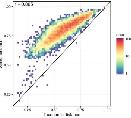
Figure 6 Correlation between taxonomic distance andk-mer based distance computed by Simka on HMP gut samples.On this density plot, each point represents one or several pairs of the gut samples. The Xcoordinate indicates the Bray–Curtis taxonomic distance, and theYcoordinate the Bray–Curtis dis-tance computed by Simka withk=21. The color of a point is function of the amount of sample pairs with the given pair of distances (log-scaled).
different distances can lead to different distributions of the samples, with some clusters being more or less discriminated (seeFig. S5). This confirms the fact that it is important to conduct analyses using several distances as suggested in (Koren et al., 2013;Legendre & De Cáceres, 2013) as different distances may capture different features of the samples.
We conduct the same experiment on the 138 gut samples from the HMP project. Arumugam et al. (2011)showed that the gut samples are organized in three groups, known as enterotypes, and characterized by the abundance of a few genera:Bacteroides,Prevotella
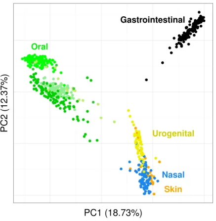
● ● ● ● ● ● ● ● ● ● ● ● ● ● ● ● ● ● ● ●● ● ● ● ● ● ● ● ● ● ● ● ● ● ● ● ● ● ● ● ●● ● ● ● ● ● ● ● ● ● ● ● ● ● ● ● ● ● ● ● ● ● ● ● ● ● ● ● ● ● ● ● ● ● ● ● ● ● ●● ● ● ● ● ● ● ● ● ● ● ● ● ● ● ● ● ● ● ● ● ● ● ● ● ● ● ● ● ● ● ● ● ● ● ● ● ● ● ● ● ● ● ● ● ● ● ● ● ● ● ● ● ● ● ● ● ● ● ● ● ● ● ● ● ● ● ● ● ● ● ● ● ● ● ● ● ● ●● ● ● ● ● ● ● ● ●● ● ● ● ● ● ● ● ● ● ● ● ● ● ● ● ● ● ● ● ● ● ● ● ● ● ● ● ● ● ● ● ● ● ● ● ● ● ● ● ● ● ● ● ● ● ● ● ● ● ● ● ●● ● ●● ● ● ● ● ● ● ● ● ● ● ● ● ● ● ● ● ● ● ● ● ● ● ● ● ● ● ● ● ● ● ● ● ● ● ● ● ● ● ● ● ● ● ● ● ● ● ● ● ● ● ● ● ●● ● ● ● ● ● ● ● ● ● ● ● ● ● ● ● ● ● ●● ● ● ● ● ● ● ● ● ● ● ● ● ● ● ● ● ● ● ● ● ● ● ● ● ● ● ● ● ● ● ●● ● ● ● ● ● ● ● ● ● ● ● ● ● ● ● ● ● ● ● ● ● ● ● ● ● ● ● ● ● ● ● ● ● ● ● ● ● ● ● ●● ● ● ● ● ●● ●● ● ● ● ● ● ● ● ● ● ● ● ● ● ● ● ● ● ● ● ● ● ● ● ● ● ● ● ● ● ● ● ● ● ● ● ● ● ● ● ● ● ● ● ● ● ● ● ● ● ● ● ● ● ● ● ● ● ● ● ● ● ● ● ● ● ● ● ● ● ● ●● ● ● ● ● ● ● ● ● ● ● ● ● ● ● ● ● ● ● ● ● ● ● ● ● ● ● ● ● ● ● ● ● ● ● ● ● ● ● ● ● ● ● ● ● ● ● ● ● ● ● ● ● ● ● ● ● ● ● ● ● ● ● ● ● ● ● ● ● ● ● ● ● ● ● ● ● ● ● ● ● ● ● ● ● ● ● ● ● ● ● ● ● ● ● ● ● ● ● ● ● ● ● ● ● ● ● ● ● ● ● ● ● ● ● ● ● ● ● ● ● ● ● ● ● ● ● ● ● ● ● ● ● ● ● ● ● ● ● ● ● ● ● ● ● ● ● ● ● ● ● ● ● ● ● ● ● ● ● ● ● ● ● ● ● ● ● ● ● ● ● ● ● ● ● ● ● ● ● ● ● ● ● ● ● ● ● ● ● ● ● ● ● ● ● ● ● ● ● ● ● ●●● ● ●● ● ● ● ● ● ● ● ● ● ● ● ● ● ● ● ● ● ● ● ● ● ● ● ●● ● ● ● ● ● ● ● Gastrointestinal Oral Urogenital Nasal Skin
PC1 (18.73%)
PC2 (12.37%)
Figure 7 Distribution of the diversity of the HMP samples by body sites.PCoA of the samples is based on the quantitative Ochiai distance computed by Simka withk=21. Each dot corresponds to a sample and is coloured according to the human body site it was extracted from. The green color shades corre-spond to three different subparts of the Oral samples: Tongue dorsum, Supragingival plaque, Buccal mu-cosa (from top to down).
DISCUSSIONS
In this article, we introduced Simka, a new method for computing a collection of ecological distances, based onk-mer composition, between many large metagenomic datasets. This was made possible thanks to the Multiplek-mer Count algorithm (MKC), a new strategy that countsk-mers with state-of-the-art time, memory and disk performances. The novelty of this strategy is that it counts simultaneouslyk-mers from any number of datasets, and that it represents results as a stream of data, providing counts in each dataset,k-mer per
k-mer.
● ● ● ● ● ● ● ● ● ● ● ● ● ● ● ● ● ●● ● ● ● ● ● ● ● ● ● ● ● ● ● ● ● ● ● ● ● ● ● ● ● ● ● ● ● ● ● ● ● ● ● ● ● ●● ● ● ● ● ● ● ● ● ● ●● ● ● ● ● ● ● ● ● ● ● ● ● ● ● ● ● ● ● ● ● ● ● ● ● ● ● ● ● ● ● ● ● ● ● ● ● ● ● ● ● ● ● ● ● ● ● ● ● ● ● ● ● ● ● ● ● ● ● ● ● ● ● ● ● ● ● ● ● ● ● ● PC1 (6.15%)
PC3 (3.53%) 25
50 75 Abundance (%)
A
Bacteroides ● ● ● ● ● ● ● ● ● ● ● ● ● ● ● ● ● ●● ● ● ● ● ● ● ● ● ● ● ● ● ● ● ● ● ● ● ● ● ● ● ● ● ● ● ● ● ● ● ● ● ● ● ● ●● ● ● ● ● ● ● ● ● ● ●● ● ● ● ● ● ● ● ● ● ● ● ● ● ● ● ● ● ● ● ● ● ● ● ● ● ● ● ● ● ● ● ● ● ● ● ● ● ● ● ● ● ● ● ● ● ● ● ● ● ● ● ● ● ● ● ● ● ● ● ● ● ● ● ● ● ● ● ● ● ● ● PC1 (6.15%) PC3 (3.53%) 0 20 40 60 Abundance (%)B
Prevotella ● ● ● ● ● ● ● ● ● ● ● ● ● ● ● ● ● ●● ● ● ● ● ● ● ● ● ● ● ● ● ● ● ● ● ● ● ● ● ● ● ● ● ● ● ● ● ● ● ● ● ● ● ● ●● ● ● ● ● ● ● ● ● ● ●● ● ● ● ● ● ● ● ● ● ● ● ● ● ● ● ● ● ● ● ● ● ● ● ● ● ● ● ● ● ● ● ● ● ● ● ● ● ● ● ● ● ● ● ● ● ● ● ● ● ● ● ● ● ● ● ● ● ● ● ● ● ● ● ● ● ● ● ● ● ● ● PC1 (6.15%)PC3 (3.53%) 1020
30 40 50
Abundance (%)
C
Ruminococcaceaeit is notable that Simka is able to scale large datasets even with the solid filter disabled as shown in the performance section. Interestingly, when applied on a low coverage dataset, namely the Global Ocean Sampling (Yooseph et al., 2007), Simka was able to capture the essential underlying biological structure with or without thek-mer solid filter (seeFig. S6). However, an important incoming challenge is to precisely measure the impact of applied thresholds together with the choice ofk, depending on the input dataset features such as community complexity and sequencing effort.
Since metagenomic projects are constantly growing, it is important to offer the possibility to add new sample(s) to a set for which distances are already computed, without starting back the whole computation from scratch. It is straightforward to adapt the MKC algorithm to such operation, but the merging step and distance computation step have to be done again. However, adding a new sample does not modify previously computed distances and only requires to compute a single line of the distance matrix, it can thus be achieved in linear time.
There is nevertheless room for improving Simka distances. For instance, recently, Břinda, Sykulski & Kucherov (2015) showed that spaced seeds can improve thek -mer-based metagenomic classification obtained with the popular tool Kraken (Wood & Salzberg, 2014). Spaced seeds can be seen as non-contiguousk-mers allowing therefore a certain number of mismatches when comparing them. Being less stringent when comparing
k-mers could lead to more accurate distances, especially for viral metagenomic fractions which contain a lot of mutated sequences.
ACKNOWLEDGEMENTS
Authors warmly thank, Olivier Jaillon and Thomas Vannier from Genoscope (CEA-IG-LAGE) and Stéphane Robin from INRA AgroParisTech for providing their technical, biological and statistical expertise, as well as feedback during the conception of this manuscript. We thank the GenOuest BioInformatics Platform that provided the computing resources necessary for benchmarking.
ADDITIONAL INFORMATION AND DECLARATIONS
Funding
This work was supported by the French ANR-14-CE23-0001 Hydrogen Project. The funders had no role in study design, data collection and analysis, decision to publish, or preparation of the manuscript.
Grant Disclosures
The following grant information was disclosed by the authors: French ANR-14-CE23-0001 Hydrogen Project.
Competing Interests
The authors declare there are no competing interests.
Author Contributions
• Gaëtan Benoit conceived and designed the experiments, performed the experiments, analyzed the data, contributed reagents/materials/analysis tools, wrote the paper, prepared figures and/or tables, performed the computation work, reviewed drafts of the paper.
• Pierre Peterlongo, Mahendra Mariadassou, Sophie Schbath, Dominique Lavenier and Claire Lemaitre conceived and designed the experiments, analyzed the data, contributed reagents/materials/analysis tools, wrote the paper, performed the computation work, reviewed drafts of the paper.
• Erwan Drezen contributed reagents/materials/analysis tools, wrote the paper, performed the computation work, reviewed drafts of the paper.
Data Availability
Supplemental Information
Supplemental information for this article can be found online athttp://dx.doi.org/10.7717/ peerj-cs.94#supplemental-information.
REFERENCES
Altschul SF, Gish W, Miller W, Myers EW, Lipman DJ. 1990.Basic local alignment
search tool.Journal of Molecular Biology215(3):403–410 DOI 10.1016/S0022-2836(05)80360-2.
Anonymous. 2011.Microbiology by numbers.Nature Reviews Microbiology9(9):628
DOI 10.1038/nrmicro2644.
Arumugam M, Raes J, Pelletier E, Le Paslier D, Yamada T, Mende DR, Fernandes GR, Tap J, Bruls T, Batto J-M, Bertalan M, Borruel N, Casellas F, Fernandez L, Gautier L, Hansen T, Hattori M, Hayashi T, Kleerebezem M, Kurokawa K, Leclerc M, Levenez F, Manichanh C, Nielsen HB, Nielsen T, Pons N, Poulain J, Qin J, Sicheritz-Ponten T, Tims S, Torrents D, Ugarte E, Zoetendal EG, Wang J, Guarner F, Pedersen O, De Vos WM, Brunak S, Dore J, Weissenbach J, Ehrlich SD, Bork
P. 2011.Enterotypes of the human gut microbiome.Nature473(7346):174–180
DOI 10.1038/nature09944.
Borg I, Groenen P. 2013. Modern multidimensional scaling: theory and applications. In:
Springer Series in Statistics. New York: Springer.
Boutin S, Graeber SY, Weitnauer M, Panitz J, Stahl M, Clausznitzer D, Kaderali L,
Einarsson G, Tunney MM, Elborn JS, Mall MA, Dalpke AH. 2015.Comparison
of microbiomes from different niches of upper and lower airways in children and adolescents with cystic fibrosis.PLoS ONE10(1):1–19
DOI 10.1371/journal.pone.0116029.
Břinda K, Sykulski M, Kucherov G. 2015.Spaced seeds improve k-mer-based
metage-nomic classification.Bioinformatics31(22):3584–3592 DOI 10.1093/bioinformatics/btv419.
Broder AZ. 1997.On the resemblance and containment of documents. In:Compression
and Complexity of Sequences 1997. Proceedings. Piscataway: IEEE, 21–29.
Cai L, Ye L, Tong AHY, Lok S, Zhang T. 2013.Biased diversity metrics revealed by
bacterial 16S pyrotags derived from different primer sets.PLoS ONE 8(1):e53649 DOI 10.1371/journal.pone.0053649.
Chao A, Chazdon RL, Colwell RK, Shen T-J. 2006.Abundance-based similarity
indices and their estimation when there are unseen species in samples.Biometrics
62(2):361–371DOI 10.1111/j.1541-0420.2005.00489.x.
Costello EK, Lauber CL, Hamady M, Fierer N, Gordon JI, Knight R. 2009.Bacterial
community variation in human body habitats across space and time.Science
326(5960):1694–1697DOI 10.1126/science.1177486.
Coveley S, Elshahed MS, Youssef NH. 2015.Response of the rare biosphere to
environ-mental stressors in a highly diverse ecosystem (Zodletone Spring, OK, USA).PeerJ
Deorowicz S, Kokot M, Grabowski S, Debudaj-Grabysz A. 2015.KMC 2: fast and resource-frugal k-mer counting.Bioinformatics31(10):1569–1576
DOI 10.1093/bioinformatics/btv022.
Deutsch P, Gailly J-L. 1996.Zlib compressed data format specification version 3.3.
Technical report.Available athttps:// www.ietf.org/ rfc/ rfc1950.txt.
Drezen E, Rizk G, Chikhi R, Deltel C, Lemaitre C, Peterlongo P, Lavenier D. 2014.
Gatb: genome assembly & analysis tool box.Bioinformatics30(20):2959–2961 DOI 10.1093/bioinformatics/btu406.
Dubinkina VB, Ischenko DS, Ulyantsev VI, Tyakht AV, Alexeev DG. 2016.Assessment
of k-mer spectrum applicability for metagenomic dissimilarity analysis.BMC Bioinformatics17:38DOI 10.1186/s12859-015-0875-7.
Fofanov Y, Luo Y, Katili C, Wang J, Belosludtsev Y, Powdrill T, Belapurkar C, Fofanov
V, Li T-B, Chumakov S. 2004.How independent are the appearances of n-mers in
different genomes?Bioinformatics20(15):2421–2428 DOI 10.1093/bioinformatics/bth266.
Genitsaris S, Monchy S, Viscogliosi E, Sime-Ngando T, Ferreira S, Christaki U.
2015.Seasonal variations of marine protist community structure based on
taxon-specific traits using the eastern English Channel as a model coastal system.FEMS Microbiology Ecology91(5):fiv034–fiv034DOI 10.1093/femsec/fiv034.
Gomez-Alvarez V, Pfaller S, Pressman JG, Wahman DG, Revetta RP. 2016.Resilience of
microbial communities in a simulated drinking water distribution system subjected to disturbances: role of conditionally rare taxa and potential implications for antibiotic-resistant bacteria.Environmental Science: Water Research & Technology
2(4):645–657DOI 10.1039/c6ew00053c.
Human Microbiome Project Consortium. 2012a.Structure, function and diversity of
the healthy human microbiome.Nature486(7402):207–214DOI 10.1038/nature11234.
Human Microbiome Project Consortium. 2012b.A framework for human microbiome
research.Nature486(7402):215–221DOI 10.1038/nature11209.
Karsenti E, Acinas SG, Bork P, Bowler C, De Vargas C, Raes J, Sullivan M, Arendt D, Benzoni F, Claverie JM, Follows M, Gorsky G, Hingamp P, Iudicone D, Jaillon O, Kandels-Lewis S, Krzic U, Not F, Ogata H, Pesant S, Reynaud EG, Sardet
C, Sieracki ME, Speich S, Velayoudon D, Weissenbach J, Wincker P. 2011.A
holistic approach to marine Eco-systems biology.PLoS Biology9(10):e1001177 DOI 10.1371/journal.pbio.1001177.
Kent WJ. 2002.BLAT—the BLAST-like alignment tool.Genome Research12(4):656–664
DOI 10.1101/gr.229202.
Koren O, Knights D, Gonzalez A, Waldron L, Segata N, Knight R, Huttenhower C, Ley
RE. 2013.A guide to enterotypes across the human body: meta-analysis of microbial
community structures in human microbiome datasets.PLoS Computational Biology
9(1):e1002863DOI 10.1371/journal.pcbi.1002863.
Legendre P, De Cáceres M. 2013.Beta diversity as the variance of community