High-pressure Raman study of graphene: a spectroscopic evidence for the diamondol

(1)

Luiz Gustavo Pimenta Martins

(2)

Universidade Federal de Minas Gerais - UFMG Instituto de Ciências Exatas - ICEx Programa de Pós-Graduação em F´ısica

High-pressure Raman study of graphene: a spectroscopic evidence for the diamondol

Luiz Gustavo Pimenta Martins

Orientador: Prof. Luiz Gustavo de Oliveira Lopes Canc¸ado

Dissertação apresentada ao departamento de F´ısica da Univer-sidade Federal de Minas Gerais, para a obtenção de T´ıtulo de Mestre em F´ısica

Área de Concentração: F´ısica da Matéria Condensada

(3)

(4)

Agradecimentos

A vida é definitivamente imprevis´ıvel (por mais contraditório que isso possa soar). Quem diria que a matéria mais odiada por mim nos tempos de colégio se tornaria o meu objeto de trabalho! Com o perdão do clichê, a caminhada foi longa até aqui e muitos foram os percalços, mas tenho a certeza de estar no caminho certo. E muitos foram os que trilharam esse caminho comigo. Portanto, a conquista de mais essa etapa é de todos vocês também.

Agradeço aos meus pais por serem o meu alicerce e a minha referência de seres verdadeira-mente humanos. À minha mãe, por ser a pessoa mais generosa e justa desse mundo, estando presente e me apoiando incondicionalmente em todos os momentos da minha vida, além de me ensinar, através de sua história de vida, o poder da determinação. Ao meu pai, pela exemplo de serenidade, equil´ıbrio e honestidade, além do carinho e empolgaçao em ter um filho cientista! Herdei de você a curiosidade, a principal caracter´ıstica de todo aquele que deseja fazer ciência. Ao meu irmão, pela amizade, preocupação e pelos conselhos ao longo da minha vida, e à sua esposa S´ılvia e ao meu sobrinho André, pelo carinho. Às minhas irmãs Ana Luiza, Marcele e Noara pela amizade e presença desde sempre. À Aparecida por cuidar de mim ao longo de todos esses anos. À Tia Eliene, Tio Ildeu e Tia Lêda por extenderem o conceito de pai e mãe.

`A Tia Queu, Tia Lula e a todos os Neves por todo apoio e pelas farras.

Agradeço à Alice, meu amor e meu porto seguro, por ser a minha maior e melhor compania sempre. Aos meus sogros, Laura e ao Orlando por abrir as portas de sua casa, (que acabou se tornando a minha 1a _{casa em BH rs), e por tudo que fizeram e fazem por mim, tendo uma} contribuição direta em diversas etapas do meu mestrado.

(5)

conheci-mento teórico aplicado em prol da geração do conheciconheci-mento. Agradeço por todas as excelentes oportunidades que me proporcionou, pelos conversas fiadas e pelos jogos do Galo!

A todo o pessoal da UFC por ter me recebido da melhor maneira poss´ıvel em todas as minhas idas e por ter viabilizado os experimentos de Raman sob alta pressão: Professores Alexandre Paschoal, Paulo Tarso, Nádia Ferreira, Antônio Gomes e Acr´ısio Lins. Sem a contribuição e dedicação de vocês, esse trabalho não teria sido poss´ıvel, literalmente. Agradecço ao Paschoal, ao Edilan, à tia Valdira e à Gabi por terem me hospedado e por me fazer sentir em casa. Agradeço à minha fam´ılia em Fortaleza: Tio Joaquim, Tia Valdira e meus primos (e respec-tivas esposas) Boris, Breno, Bráulio, Bruno e Gabriela, por terem feito minhas idas a Fortaleza mais divertidas.

I would like to thank Professor Jing Kong for hosting me in the NanoMaterials and Electronics Group (NME) in MIT where all the samples of this work were produced, also for being the perfect example of brightness and kindness. I also would like to thank all people from the NME group for all support and fun I had during my time in MIT. I would like to thank Professor Mildred Dresselhaus for the fruitful discussions and for the example of how science can be used to promote social equality. Ao Paulo T. Araújo (Simpa) pelas orientações acadêmicas e não acadêmicas.

Aos Amigores, aos Mansos, aos amigos do Dom Bosco, da EQ, aos amigos do Vale do Aço, aos do Vale do Aço que estão em BH e aos amigos que não se encaixaram em nenhuma das catego-rias anteriores: vocês fazem minha vida muito melhor. Em especial gostaria de agradecer aos meus amigos/irmãos Matheus, Ricardo, Carlos Alberto (Gurta), Transitions (Tiago), Amigor, Neto e Bruninha que me deram força durante um dos momentos mais dif´ıceis da minha vida. Serei eternamente grato a vocês.

`A Rosana, por sempre me indicar o caminho certo e por me explicar o Princ´ıpio da Incerteza na pr´atica rs.

Aos meus amigos do Departamento de F´ısica da UFMG, Paloma (Cabec¸a), Paula Favela, Thales e Paulim que fizeram esses dois anos de mestrado muito melhores. Ao Lucas Cpamm pelas conversas e apoio para as aplicac¸oes de doutorado nos EUA.

(6)

Ao Mario Sérgio pela paciência ao responder as milhares de dúvidas das mais diversas áreas da F´ısica que já lhe perguntei, além das discussões em conjunto com o colega Matheus Matos, que contribuiram diretamente para esse trabalho.

Ao Ado pela visão de correlação entre ciência e inovação e a todas as discussões e contribuições diretas a esse trabalho.

Ao Chubaka pelos galhos quebrados e pelas contribuio¸es a esse trabalho.

A todos os colegas do Laborat´orio de Nano-Espectroscopia pela convivˆencia.

A todos os professores do Departamento de F´ısica da UFMG que contribuiram com a minha formac¸˜ao.

A todos os outros funcionários do departamento de F´ısica da UFMG, ao pessoal da limepza, das secretarias e às bibliotecárias. Em especial à Shirley por sempre me ajudar em tudo que precisei.

Aos Programas de Pós Graduação em F´ısica da UFMG e da UFC e à Rede de Nano-Instrumentação em Espectrosocpia Óptica por financiar minhas idas à UFC.

Ao CNPq e ao povo brasileiro pelo aux´ılio financeiro.

(7)

Resumo

Nessa dissertação investigou-se o efeito de altas pressões sobre o espectro Raman de bicamadas de grafeno CVD depositadas sobre substratos de Teflon. Para tanto, foi utilizada uma célula de bigorna de diamante (DAC) com água como meio transmissor de pressão. Os espectros foram obtidos com excitação em 488 nm e 532 nm. Inicialmente foi feito um estudo detalhado das propriedades eletrônicas e vibracionais do grafeno, bem como da interação entre essas. Em seguida investigou-se o processo de Espalhamento Raman e as origens da banda G no grafeno, assim como as perturbações causadas a essa banda por efeitos de dopagem e distorção (strain). Obteve-se um valor númerico para a dispersão da banda G em função da pressão igual a 5 cm−1_/_{GPa através de uma combinação de análise teórica e resultados experimentais. Este valor}

está de acordo com observações experimentais para amostras de grafeno suspenso sujeitas a altas pressões. Os resultados do experimento fornecem fortes evidências da ocorrência de uma transição de fase de uma estrutura sp2para uma estrutura h´ıbridasp2₋sp3ocorrida entre 5₋6 GPa. A transição é revers´ıvel com a redução da pressão. As principais evidências para essa transição foram o deslocamento para maiores frequências (ωG) e a diminuição da largura a meia altura da banda G (ΓG) com o aumento da energia de excitação do laser e a mudança de regime da curvaωG× P. Foi proposto que a estrutura com hibridização sp3 tem origem na formação do diamondol, um diamante hidroxilado bidimensional formado por duas camadas de átomos de carbono hibridizadas em sp3. Foi levantada a hipótese de que a camada superior sofreu uma hidroxilação entre 5₋6 GPa, seguida de um “descolamento” do diamondol do substrato de Teflon em 9.5 GPa, resultando em uma hidroxilação da camada inferior. Essa hipótese

(8)

da curva ωG × P, nem mudança de ΓG com excitação do laser em nenhuma das amostras, o que corrobora com a hipótese do diamondol. Observou-se também o surgimento de uma nova banda em torno de 620 cm−1 _{a pressões superiores a 1 GPa e as poss´ıveis origens dessa banda}

foram discutidas. Se a hipótese do diamondol for confirmada, esse trabalho irá abrir novas perspectivas para a s´ıntese de materiais bidimensionais através de experimentos de alta pressão.

(9)

Abstract

In this dissertation, the effect of high pressures on double transferred CVD graphene sitting on a Teflon substrate were investigated via Raman spectroscopy in a diamond anvil cell (DAC) using water as the pressure transmitting media (PTM). The Raman spectra were acquired with both 488 nm and 532 nm excitation light sources. Initially, a detailed study of the electronic and vibrational properties of graphene, as well as the interaction between them, was performed. Then, an investigation on the origin of the G band in graphene was carried out, as well as the perturbations to this band caused by strain and doping. A numerical value for the slope of G band frequency with pressure (∂ωG/∂P) of 5 cm−1/GPa was obtained via a combination of theoretical analysis and experimental data. This value agrees with experimental observations for free-standing graphene samples subjected to high pressures. The results provide strong evidence of a phase transition from asp2to a sp2₋sp3mixed structure at 5₋6 GPa, reversible upon pressure release. The main evidences were the blueshift of theGband frequency (ωG) and the decrease of G band’s full width at half maximum (ΓG) with increasing excitation energy, and the change of r´egime of theωG×Pcurve. Based on the experimental data, we propose the formation of diamondol, a 2D hydroxylated diamond consisting of two layers of sp3 carbon. We hypothesized that the top layer was hydroxylated at 5₋6 GPa, followed by a detachment of the diamondol from the Teflon substrate at 9.5 GPa, which in turn led to the hydroxylation

(10)

for this band were proposed. If the diamondol hypothesis is confirmed, this work will open up directions for synthesizing new 2D materials with remarkable properties via high pressure experimental routes.

(11)

Introduction

High-pressure experiments conducted with graphite at room temperature using different pres-sure transmitting media (PTM) indicates that this material goes through a phase transition be-tween 10-20 GPa [1, 2, 3,4, 5,6]. The new phase, as well as its properties, could be detected through different experimental techniques. High-pressure in situ X-ray diffraction experiments indicate new additional peaks around 14 GPa [1]. Inelastic X-ray scattering reveals that half of the π bonds between graphite layers is converted to σ bonds at 17 GPa [2]. Raman

mea-surements and x-ray diffraction studies indicate an abrupt broadening of G band’s full-width at half-maximum, Γ_G, around 10 GPa and the subsequent loss of that signal around 14 GPa, coinciding with the loss of graphite diffraction peaks at that same pressure [3]. The abrupt broadening ofΓ_G was assigned to the formation ofsp3 bonds. Optical observations of graphite single crystals indicate the formation of a transparent phase at 18 GPa [4] and a drastic drop on its reflectivity around 16 GPa [5]. Electrical resistivity measurements reveal a rapid increase in resistivity for pressures above 15 GPa [6]. The new phase is superhard, capable of indenting the diamond used in the high-pressure apparatus [2]. The scattered values for the transition pressure found in literature reveals that the phase transition is very sensitive to the nature of the starting material as well as to the nature of the pressure applied to the sample [1]. Depending on the maximum pressure reached, the transformation is reversible [1,2,3,4] showing large hysteresis [1, 3, 4]. Different models of the structure of this new phase were proposed to explain these experimental results [1, 2, 7,8, 9,10], being generally accepted that this new phase is formed by the appearance ofsp3bonds between graphite layers during compression [11].

(15)

on the properties of these materials. Ressonant Raman Spectroscopy (RRS) has proven to be an efficient technique to determine these materials’ properties [16,17], therefore RRS has been the main chosen technique to investigate the effects of applied pressure on graphene. A phase transition in graphene nanoplates around 15 GPa [11] was identified by Raman Spectroscopy. Similarly to graphite, the transition was related to an abrupt broadening ofΓG. X-ray measure-ments in few layer graphene indicated the loss of the diffraction peak with increasing pressure for an interlayer distance of 2.8 Å[12]. The effects of strain and doping from the PTM as the pressure is increased were also studied trough RRS. An important parameter in these studies is the G band’s position (ωG) since it is directly affected by strain and doping. The derivative ofωGwith respect to the pressure (∂ωG/∂P) give information about how these two parameters evolve with increasing pressure. However, there is no agreement regarding the contributions of doping and strain to the displacement of ωG in literature data [13, 14, 15]. Nicolle et al. [13] considered both factors and reported giant doping levels in graphene and bilayer graphene im-mersed in alcohol mixture. Filintoglou et al. [14] suggested that any pressure-induced doping is too small to influence the pressure response of graphene, which is rather determined by the compressibility of the substrate and the graphene interaction with the substrate and the PTM. Proctor et al. [15] also considered only mechanical effects to explain the pressure response of graphene, mentioning that doping effects could explain the difference in the observed behavior of graphene and graphite under pressure. The only common agreement in all these works is that

∂ωG/∂Pis positive, and its value depend on both, number of layers and PTM.

An interesting effect involving graphene under high-pressure was observed by Barboza et al. [18]. In their work, ab initio calculations show that two layers of graphene under compression can be turned to a 2D hydroxilated diamond, called diamondol, if the top layer is covered with hydroxyl groups (Fig.1).

(16)

The top layer becomes fully sp3 hybridized with the four first neighbors, while the bottom layer has a carbon atom per unit cell, with only three neighbors, leaving a dangling bond. This periodic array of dangling bonds gives rise to an important feature of the electronic dispersion close to the Fermi level: the two spin polarized bands, indicated by red and blue curves in Fig.2. As a result, an energy gap of 0.6 eV opens up and the system acquires a magnetic moment of one Bohr magneton per unit cell, making diamondol a 2D ferromagnetic semiconductor.

Figure 2: Electronic dispersion (left) and electron density of states for diamondol (right). Figure taken from [18].

A strong evidence of the experimental realization of the diamondol hypothesis was obtained through electric force microscopy (EFM) experiments. EMF was used to both inject and moni-tor charges and to apply pressure on mono-, bi-, and multi-layer graphene, while the water con-tent on the sample surface was controlled by regulating the temperature of the experiment. It was observed a strong inhibition on the charging efficiency for bilayer and multilayer graphene as the tip pressure increased, while monolayer charging was pressure-independent [18].

All these works show that there are many opened questions and a vast field to be explored in-volving graphene under high pressures. In this context, in order to observe a phase transition involving the formation of sp3carbon, double layer CVD graphene was subjected to high pres-sures in a diamond anvil cell (DAC), while the Raman spectra was acquired using water as a pressure transmission medium (PTM).

(17)

classical treatment of the normal modes of vibration in graphene, and an introduction to the (quantum mechanical) concept of phonon. We finish this chapter by studying the interaction between the electrons and the vibrating lattice (the electron-phonon interaction) which is, ac-cording to the author’s opinion, the most important single concept to understand the Raman spectrum of graphene. Chapter2covers the Raman process through a quantum mechanical ap-proach. Chapter3is the key chapter of this dissertation, providing the basis for understanding the experimental results. The perturbations to the G band from mechanical strain and doping are introduced. An important result obtained in this chapter is a value for the slope of the G band frequency with pressure (∂ωG/∂P), which was obtained via a combination of theoretical anal-ysis and experimental data. This value agrees with experimental observations for free-standing graphene samples. Chapters4 to6 cover the original contribution of this dissertation. Chap-ter 4 provides a detailed description about the sample fabrication process, covering both, the synthesis of graphene by the chemical vapor deposition (CVD) technique, and the direct trans-fer of graphene onto Teflon substrates. Chapter5covers the high-pressure Raman experiment. The results indicate that graphene undergoes a phase transition to a mixedsp2₋ sp3phase. To explain the results, we discuss how the Raman data is consistent with the hypothesis that the two layer graphene has became a diamondol under high-pressure conditions, and using water as PTM. We also report on the appearance of a new Raman band centered at_∼620 cm−1_under

(18)

Chapter 1 Graphene

1.1 Carbon atom: electronic hybridization

The electronic configuration of a carbon atom in its ground state is 1s2 _2s2 _2p2_{, with four} va-lence electrons at the 2s and 2p levels, and two core electrons at the 1s level. Based on its electronic configuration, it is physically sound that carbon should be chemically divalent, with two 2pelectrons involved in chemical bonds, the other two 2selectrons being chemically inert. However, monoatomic carbon materials are found in several forms in which carbon atoms are covalent bonded to two, three, and four neighboring carbon atoms as in carbynes [19], graphene, and diamond respectively. The reason why carbon atoms are able to form such distinct struc-tures is related to their many possible electronic configurations, which is known as hybridization of atomic orbitals [20]. Hybridized orbitals are constructed from linear combinations of atomic orbitals, the later serving as basis functions to the former. The superposition of these hybridized orbitals with neighboring atoms gives rise to different types of chemical bonding, depending on the hybridization of the central atom.

(19)

the Laguerre polynomials, and an angular componentYl,m(θ, φ) corresponding to the spherical harmonics, on the form

ψn,l,m=Rn,l(r)Yl,m(θ, φ). (1.1)

Since chemical bonding involves only valence electrons, we are concerned with theψ2,l,mstates. The radial components of the 2s and 2p wave functions are equal in magnitude, and may be omitted at this point [22]. The angular components of the atomic orbitals sand pi (i = x,y,z) are given, respectively, as:

s : Y0,0(θ, φ)= √1 4π

pz: Y1,0(θ, φ)=i

r

1 4πcosθ

px,y : Y1,_±1(θ, φ)= ∓i

r

3 8πsinθe

±φ_.

(1.2)

The formation of covalent bonds in molecules or solids generates a drop on the total energy due to the overlap of the electron wave functions, giving rise to the molecular orbitals, in case of molecules, or electronic bands, in case of solids. In this case, the extra energy can be suf-ficient to promote a 2selectron into a 2porbital, (this energy being approximately 4.2 eV for carbon atoms). However, the necessary extra energy is only achieved if the overlap of the wave functions between neighboring atoms is maximal. Such a condition is satisfied when the rel-ative position between the central and neighboring atoms assume those directions for which the atomic wave functions take on maximal values. These values can be achieved through the process of hybridization and the larger they are, the stronger the bond is.

In order to construct the hybridized states, we need to choose a set of basis functions. Rather than taking theψl,m(θ, φ), it is more convenient to choose their orthonormalized linear

combina-tions:

i√2π[ψ1,1(θ, φ)−ψ1,₋1(θ, φ)]=

√

3 sinθcosφ

i√2π[ψ1,1(θ, φ)+ψ1,₋1(θ, φ)]=

√

3 sinθsinφ

−i√4πψ1,0(θ, φ)=

√

3 cosθ,

(20)

and therefore, the basis functions can be represented as

|2si=1

|x_i= √3 sinθcosφ, _|y_i= √3 sinθsinφ, _|z_i= √3 cosθ. (1.4)

Finally, the hybridized orbital can then be constructed as

ψ(θ, φ)= a+ √3(bsinθcosφ+csinθsinφ+dcosθ) (1.5)

or in Dirac’s notation

|ψ_i=a_|s_i+b_|x_i+c_|y_i+d_|z_i, (1.6)

with_|s_i,_|x_i,_|y_i, and_|z_idefined in (1.4). We now look for a set of real numbers (a,b,c,d) that will

maximizes the norm of_|ψ_i. In other words, we must find the directions for whichψassumes its

maximum value (ψmax). Since |ψiis the angular component of the total wave function, it must be normalized

hψ_|ψ_{i ≡}

Z

| hψ_|ψ_i2_|dΩ =4π

= a2_hs_|s_i+b2_hx_|x_i+c2_hy_|y_i+d2_hz_|z_i

(1.7)

withdΩ being the differential solid angle element. It follows that, to satisfy the normalization condition1.7, we must have

a2+b2+c2+d2 = 1 (1.8)

We thus need to maximize the function ψ(θ, φ) with the restriction given from equation1.8 .

This can be solved by the method of Lagrange Multipliers. For that, we must solve the set of equations

∇ψ =λ_∇g, (1.9)

withλbeing the Lagrange multiplier, andgthe restriction

(21)

Figure 1.1: Coordinate system for finding directions of maximum value for hybridized wave functions of a carbon atom. The carbon atom is placed at the origin coinciding with the center of a side two cube. Figure adapted from [22].

Let us place the origin, and the central carbon atom as well, at the center of a cube of side 2 and coordinate axes parallel to its edges. We are going to assume that, for a specific_|ψ_i,ψmaxis reached along the diagonal direction of the cube (1,1,1), (see Fig. 1.1). Thus we need to find

(a,b,c,d) for that specific_|ψ_i. Along the (1,1,1) direction, we have

sinφ= cosφ= _√1

2, cosθ= 1

√

3, sinθ=

r

2

3, (1.11)

so that

|x_i=1,_|y_i=1,_|z_i=1. (1.12)

It follows that, by considering the conditions (1.10) and (1.12), Eq. 1.9can be solved to

a= b= c=d. (1.13)

(22)

a= 1

2. (1.14)

Thus substitution of (1.14) into (1.6) determines the first orbital

|sp3₁_i= 1

2(|si+|xi+|yi+|zi), (1.15) for whichψ assumes the maximum valueψmax. Next, we need to find a set of three orthonor-mal orbitals orthogonal to _|sp3₁_i. In other words, we need to find a basis that spans the three dimensional subspace orthogonal to_|sp3₁_i. Let us assume that these orbitals have the form

|sp3_i_i= α_|s_i+β_|x_i+γ_|y_i+δ_|z_i. (1.16)

The orthogonality with_|sp3₁_iimplies

hsp3_i_|sp3₁_i= 0_→α+β+γ+δ =0. (1.17)

Equation1.17, combined with the normalization condition, gives the necessary ingredients for the determination of the three orbitals. Since they are not uniquely determined, one possible solution is on the form

|sp3₂_i= 1

2(|si+|xi − |yi − |zi)

|sp3₃_i= 1

2(|si − |xi+|yi − |zi)

|sp3₄_i= 1

2(|si − |xi − |yi+|zi).

(1.18)

The norms of the wavefunctions _|sp3_i_i (i = 1,2,3,4) take their maximum values along the

(23)

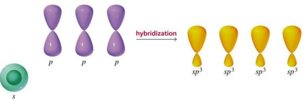
Figure 1.2: Illustration of the process ofsp3hybridization. A sorbital combines with three porbitals,

resulting in four hybridizedsp3orbitals. Figure taken from [23].

the angular component of the so-called sp3 orbitals of the carbon atom. In this configuration, the 1sorbital combines with three porbitals resulting in four hydridized orbitals, as illustrated in Fig.1.2.

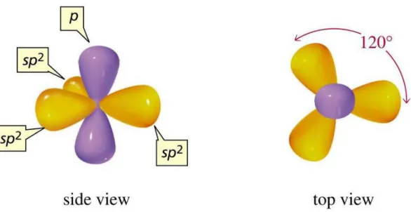
Another option is to take the linear combination of a 2s orbital with two 2p orbitals, for ex-ample 2px and 2py, whereas the remaining porbital, pz in this case, remains unchanged. This configuration of the carbon atom is calledsp2hybridization and can be achieved if one repeats the aforementioned procedure for a smaller basis including only functions_|s_i, _|x_iand_|y_i. The calculations are straightforward and will not be reproduced here. The result is

|sp2₁_i= _√1 3|si+

√

2_|x_i

|sp2₂_i= _√1 3|si −

1

√

6|xi+ 1

√

2|yi)

|sp2₃_i= _√1 3|si −

1

√

6|xi − 1

√

2|yi).

(1.19)

(24)

Figure 1.3: Illustration of the sp2 hybridized orbitals. The sp2 orbitals lie in the x-y plane forming

angles of 120◦_{to each other while the}_p_z_{orbital lies in the}_z_{axis. The}_sp2_{orbitals are responsible for the} formation ofσbonds, while the pzorbitals are responsible for formation of theπbonds. Figure taken

from [23].

1.2 Electronic structure of graphene: the tight binding method

In Sec.1.1 we linearly combined atomic orbitals of a carbon atom in order to obtain new hy-bridized atomic orbitals. In this section we are going to somewhat extend this procedure for a crystal, and the method we will employ is called the tight binding. In this method, the wave function of the crystal is constructed by a linear combination of the atomic orbitals of its con-stituents, with the coefficients of the expansion given by the Bloch Theorem. The tight binding method is one of the simplest methods for calculating electronic structures of solids and it is of great practical utility.

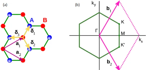
In order to determine the electronic structure of graphene using this method, the first step is to specify the unit cell and the unit vectorsai~ (i = 1,2) of the crystal lattice. In graphene, the

carbon atoms are disposed in a hexagonal lattice as show in Fig.1.4(a). The graphene Bravais lattice is triangular , and the lattice vectors are given [in the x,y basis defined in Fig.1.4(a)] as

~

a1 = a₂(

√

3,1), a~2 = a₂(

√

3,₋1), (1.20)

(25)

Figure 1.4: In (a): direct lattice with primitive vectorsai~ and first neighboursδ~i. In (b): recip-rocal lattice with high symmetry pointsΓ,K andM. Figures taken from [24].

The next step is to specify the Brillouin zone and the reciprocal lattice vectors, _bi~ _(i ₌ ₁_,_{2) ,}

followed by the selection of high symmetry points and lines. For a two dimensional crystal, the reciprocal lattice vectors can be determined by

~

bi =

2π(ˆn_×a~j) ˆ

n_·(a~j×ai~)

, (i, j=1,2) (1.21)

where ˆnis the vector normal to the plane containing the vectorsa~1anda~2. The reciprocal lattice is also triangular, with lattice vectors:

~

b1 = 2π a (

1

√

3,1), b~2 = 2π

a ( 1

√

3,−1), (1.22)

corresponding to a lattice constant of 4π/√3a. The Brillouin zone is represented by the hexagon

in Fig.1.4(b). The three high symmetry pointsΓ,Kand Mare indicated, corresponding to the center, the corner and the center of the edge respectively. Their coordinates are:

Γ =(0,0), K = 2π a (

1

√

3, 1

3), M =( 2π

√

3a,0). (1.23)

Theπelectrons are the valence electrons which are the relevant ones for the transport properties;

(26)

Figure 1.5: Representation of the Bloch orbitals in a 1D lattice. The top shows the pz wave-functions (actually its square modulus) of individual carbon atoms, the middle shows (the real part) of the phaseei~k·~rof of the Bloch orbitals and the bottom shows the amplitude of the Bloch orbitals.

φi(~k,~r)= 1

√

N

X

~

R

ei~k·~rφi(~r−R)~ , (i=1, ...,n), (1.24)

where _R~ _{is the position of the atom,} _φ_i _{denotes the atomic wave function index by} _i _and _n_is

the number of the wavefunctions in the unit cell. The functionφi(~r−R) represents an atomic~ wave function centered at position _R~ _{in the lattice. As all lattice vectors are being swept by}

the index _R~ _{in the summation, the total wave function}_φ_i₍~_k_,~_{r) will be a linear combination of}

all atomic wave functions of the crystal. These functions are weighted by the factorei~k·~r, which modulates the crystal wavefunction as pictured in Fig.1.5for a 1Dlattice. In case ofπelectrons

in graphene there are two wavefunctions in the unit cell, namely the two 2pzorbitals, associated with the two inequivalent carbon atoms AandB. Thus, there will be two functions,φA andφB, which are formed by combining 2pzorbitals betweenAandBatoms respectively. Let us place the origin of ourx,ycoordinate system in atom A, as illustrated in Fig. 1.4(a). In this case, we have

φA(~k, ~R)= 1

√

N

X

~

R

ei~k·~rφA(~r−R)~ , R~= n1a~1+n2a~2, (1.25)

wherea~1 anda~2 are the primitive vectors defined in (1.20). To construct φB we use the same coordinate system, choosing a vector_B~_{that connects A atoms to B atoms. The aid of this vector}

(27)

atom, only the orbitals of A atoms are summed. The trick of introducing the ₋~_B_{vector in the}

argument of the wavefunction during the summation, changes the summation over A atoms to the summation over their nearest neighbors B atoms.

φB(~k, ~R)= 1

√

N

X

~

R

ei~k·~rφB(~r−B~−R)~ , B~ = 2a

√

3,0

!

(1.26)

To obtain the one-electron energy eigenvaluesEi(~k) the secular equation must be solved [20]

|H−ES|= 0. (1.27)

TheH andS matrices are the transfer integral matrix and the overlap integral matrix, respec-tively, whose matrix elements are defined as are defined as

Hi j(~k)= hφi|H|φji, Si j(~k)= hφi|φji, (i, j= 1, ...,n). (1.28) Thus, bothHandSaren_×nmatrices and the solution to Eq.1.27gives all n eigenvaluesEi(~k). The (2_×2) transfer integral matrix is obtained by substituting Eq. (1.24) into Eq. (1.28). We are going to first calculate the diagonal terms,

HAA =_hφA|H|φAi= 1 N

X

~

R, ~R′

ei~k·(R~−R~′)_hφA(~r₋R~′)_|_H_|_φA(_~_r₋R)~ _i

= 1 N

X

~

R=R~′

hφA(~r−R~′)|H|φA(~r−R)~ i

+ 1 N

X

~

R=R~′_±a~i

e±i~k·a~i

hφA(~r−R~′)|H|φA(~r−R)~ i

+(terms in whichR~₋R~′ >2a~i).

(1.29)

(28)

H(~r)=₋ ℏ 2m∇2+

X

i

Uatomic,i(~r)+ ∆Ui(~r) i= A,Bwhere Uatomic,A(~r)=Uatomic,A(~r+R);~ ∆UA(~r)= ∆UA(~r+R)~

Uatomic,B(~r)=Uatomic,B(~r+B~+R);~ ∆UB(~r)= ∆UB(~r+B~+R)~ .

(1.30)

The functionsUatomic,i and∆Ui(~r) are the potential energy functions associated with the inter-action between the electron and the carbon atoms (A and B), and the correction to that energy at that position, respectively. The∆Ui term contains all corrections to the atomic potential to reproduce the full periodic potential of the crystal. The functions φi(~k,~r) are well localized at the atomic positions, with its amplitude being very small when~rexceeds a distance of the order of the lattice constant. Therefore the first term of Eq. 1.29yields:

1 N

X

~

R=R~′

hφA(~r−R~′)|H|φA(~r−R)~ i= 1

N

X

~

R=R~′

Z

φA(~r−R~′)HφA(~r−R)d~ ~r= ε∗2pz

(1.31)

where each integral has only an appreciable value on the vicinity of each atom. Note thatε∗

2pz is

not simply the electron energy for the free carbon atom, because the Hamiltonian contains the ∆Ui terms. We can use the same approximations to get that HBB = ε∗_2p_z. For the off-diagonal matrix elements we are going to consider only the three nearest neighbor B atoms relative to an A atom. The relative positions between the central atom A and the three nearest neighbors B are denoted by~δ1,~δ2, and~δ3. Following these definitions, the off-diagonal matrix elementsHAB are evaluated as

HAB =_hφA|H|φBi = 1

N

X

~

R, ~R′

ei~k·(R~−R~′)_hφA(~r−R~′)|H|φB(~r−B~−R)~ i

= 1 N

X

~

R=R~′_±~_δ_i

ei~k·R~i

hφA(~r−R~′)|H|φB(~r−R)~ i, i=1,2,3

=γ(ei~k·δ~1 ₊_ei~k·δ~2 ₊_ei~k·δ~3₎₌_γ_f₍~_k)_.

(1.32)

whereγis the nearest neighbor transfer integral. In the graphene case,γhas the form

(29)

f(~k)=eikx√a₃

+2e−ikx₂a√₃ _cos kya

√

3. (1.34)

Since H is Hermitian (H = H†), we have HBA = HAB∗, where the symbol _∗ stands for the complex conjugate. To calculate the overlap integral matrixS, we use the fact thatSAA =SBB = 1, assuming that_|φAiand|φBiare normalized. To calculate the off-diagonal elements ofSwe can repeat the same method used to obtainHi j. In this case, we haveSAB = s f(~k)= SBA∗with

s=_hφA(~r−R)~ |φB(~r−R~+δ~i)i, (i=1,2,3). (1.35) The final form of the matricesHandSare

H=         ε∗

2pz γf(

~_k)

γf(~k) ε∗

2pz       

, S=

       

1 s f(~k) s f(~k) 1

      

. (1.36)

Solving the Secular Equation (1.27), with HandS being given by Eq. 1.36, the eigeinvalues E(~_{k) are obtained as a function of}~_k₌ ₍_k~_x_{, ~}_k_y₎

E(_k~_x_{, ~}_k_y₎₌ ε∗2pz ±γw(

~_k)

1_∓sw(~_k) , (1.37)

with the functionw(~_{k) given by:}

w(~_k)₌_|_f₍~_k)_|2 ₌

s

1+4cos

√

3kxa 2 cos

kya

2 +4 cos2 kya

2 . (1.38)

The solution with+ signs in the numerator and₋sign in the denominator gives theπ bonding

energy band, while the other solution gives theπ∗ _{anti-bonding energy band. A plot of the}

en-ergy dispersion relation throughout the first Brillouin zone of graphene is displayed in Fig. 1.6 (b). Figure1.6 (c) shows the energy dispersion relations along the high symmetry axes along the perimeter of the triangle ΓK M. The tight binding method is not sufficient to completely determine electronic structures of crystals because the parametersε∗

2pz, γ and sneed to be

de-termined either from first principle calculations or experimentally. Here we use the parameters

ε∗

(30)

Figure 1.6: (a) Graphene lattice in real space. (b) The energy dispersion plot of π electrons

in graphene over the first Brillouin Zone. (c) The energy dispersion along the high symmetry directions along theΓK M trajectory. (d) The Dirac Cone near theK(K′) points. Figure taken from [25].

Since there are two π electrons per unit cell, for undoped graphene the lower π band is

com-pletely occupied. The upperπ∗_{and the lower}_π_{bands touch each other at the}_K _{points, through}

which the Fermi energy passes. The density of states at the Fermi level is zero, therefore graphene is a zero-gap semiconductor. This comes from the symmetry requirement that the two carbon atoms at sites A and B are equivalent to each other. If the A and B sites had different atoms such as B and N, which is the case for boron nitride, the site energyε∗

2pz would be

dif-ferent for B and N, and therefore the calculated energy dispersion would show an energy gap betweenπ and π∗ _{bands [}₂₀_{]. The energy dispersion close to the}_K _{point is exhibited in Fig.}

1.6 (d). Note that the energy dispersion around this point takes the form of a cone, called the Dirac Cone. The linear dispersion of the πelectrons around the K point is the responsible for the remarkable optical and transport properties of graphene.

1.3 Vibration modes in Graphene

(31)

a force-constant model to obtain the eigenfrequencies ω(~k) of the normal modes, where~k is in the first Brillouin Zone. As a result, we will obtain the phonon dispersion relation of ω(~k)

along high symmetry directions of the BZ. The concept of phonon is associated with quantum mechanics and will be explained at the end of this section. Until that point, our approach lies completely within classical theory, with all “quantumness” hidden in the spring constants.

1.3.1 Dynamical matrix

The equilibrium position of theith atom in a lattice is given by the lattice vectorR~i, while its instantaneous position of it is represented by _R~′

i. We start by writing the Lagrangian in the harmonic approximation:

L = 1

2 X i mi ˙ ~

R′_i

2

− 1₄X

i,j K(i j)

R~

′

i−R~′j−∆R~i j

2

,∆R~i j =R~i−R~j. (1.39)

Heremi is the mass of theith atom andK(i j)is the force constant tensor between theithand jth atoms, which is represented by a 3_×3 matrix. The sum over jis taken, in principle, over all neighbors of theithatom in the lattice.

It is useful to define the relative displacement of the ith _atom_~_u_R_~ i

or, in a more condensed notation,~ui =R~′i−R~i. Using this notation we have

~

R′i−R~′j =~ui−~uj+

~

Ri₋R~j

=~ui₋~uj+ ∆Ri j~ and R~˙′_i =~ui˙ .

(1.40)

By substituting 1.40 intto 1.39 we get the Lagrangian expressed in terms of the relative dis-placements on the form

L ₌ 1

2 X i mi ~u˙i

2

− 1₄X

i,j K(i j)

~ui−~uj

2

. _(1.41)

(32)

mi~u¨i =

X

j

K(i j)_~_u_j₋_~_u_i (i= 1, ...n), (1.42)

wherenis the number of atoms in the unit cel. The sum over jis usually taken over only a few neighbor distances relative to theithsite, which for graphene has been carried out up to the 4th nearest-neighbor interactions [20].

A travelling wave is one solution to Eq. 1.42, thus a more general solution can be chosen by representing~ui as a superposition of traveling waves with polarization~uk. In other words, we can perform a Fourier transform of the displacement of theithatom with the wave number~kto obtain the normal mode displacements~u(i)_~

k

~ui = 1

√

N

X

~_k

e−i _~

k·R~i−ωt

~

u(i)_~

k or ~u (i)

~_k =

1 √ N X ~ Ri ei ~

k′_·~Ri−ωt

~ui, (1.43)

where the sum is taken over all N wave vectors~k in the first Brillouin zone, with N being the number of unit cells in the solid. The crucial point is to understand that the travelling wave1.43 is not simply a mathematical solution to the differential equation1.42, but it actually represents a collective motion of all atoms in the lattice. This can be clearly seen in Fig. 1.7 , which represents a normal mode associated with a travelling wave with wave vectork. If one fix their attention to a single position_R~_i_{, the displacement of the atom at that position}_~_u_i_{, describes an}

harmonic motion as the wave passes trough it. Now if one pay attention to different positions in the lattice, what will be seeing is that each atom is moving up and down performing an harmonic oscillation, although the overall result is a collective motion, along the horizontal direction in this case, consisting of a normal mode.

Taking the second derivative of~ui in Eq. 1.43, and assuming the same eigenfrequencies ωfor all~ui, we have ¨~ui =₋ω2~ui. The substitution of this relation in Eq. 1.42yelds

        X j

K(i j)₋_m_i_ω2(~k)

        X ~ k

e−i~k·R~i_u(i)

~_k =

X

j

K(i j)X

k

e−i~k·R~j_~_u(j)

~_k . (1.44)

Next, if we multiply both sides of Eq. 1.44byeik~′·R~i, and perform a summation on_R~

(33)

Figure 1.7:Normal mode associated with a travelling wave.         X j

K(i j)₋_m_i_ω2(~k)

        X ~_k X ~ Ri ei ~

k′−~k

·R~i

u_~(i) k

=X

j

K(i j)X

k X ~ Ri ei _~

k′−~k

·R~i

ei~k· _~

Ri−R~j

~

u(_~j) k .

(1.45)

Now we use the orthogonality condition in the continuum~_k_{space [}₂₀_]

X

~

Ri

ei _~

k′−~k

·R~i

=Nδ_k~′~_k, (1.46)

to have         X j

K(i j)₋_miω2(~k)I

       u (i)

~_k −

X

j

K(i j)_e~k·∆Ri j_u(j)

~_k =0, (i= 1, ..,n), (1.47)

(34)

        X j

K(1j)₋_m₁_ω2(~k)I

       u (1)

~_k −

K(11)_e0_u(1)

~_k +K

(11′₎

e~k·∆R11′_u(1′)

~

k +...

−

K(12)_e~k·∆R12_u(2)

~

k +

K(12′)_e~k·∆R12′_u(2′)

~_k +...

+...₋K(1n)_e~k·∆R1n_u(n)

~_k

+K(1n′)_e~k·∆R1n′_u(n′)

~_k +...

(1.48)

The summation inside each parenthesis is taken for equivalent atoms. It means that the coordi-nates_R~₁_and_R~₁_′ _{differ only by a lattice vector. In fact, because the} _j_and _j′_{sites are equivalent}

to each other, we can show thatu_~j

k is equal tou j′

~

k. To prove this we go back to the definition of u_~j

k in Eq.1.43:

~u_~(j′) k = 1 √ N X ~

Rj′ ei

_~ k·R~j′−ωt

~

uj′, R~_j−R~_j′ = 3

X

i=1

ni~ai

= _√1 N

X

~

Rj−Pni~ai

ei _~

k·R~j−ωt

~

u_~ Rj−Pni~ai

e

−i~k·Pni~ai

| {z } 1

= _√1 N X ~ Rj ei _~

k·R~j−ωt

~uj =~u_~(j) k .

(1.49)

It is important noticing that, in (1.51), the wavevector k can be written as a linear combination of primitive reciprocal vectors, that is,~_k ₌ P3

i=1ni~bi, ~bi being a basis vector and ni an integer. Here we have used the propertyai·bj =2πδi j. Thus we can rewrite Eq. 1.48as

                X j

K(1j)₋_m₁_ω2(~k)I

       −

K(11)_e0+K(11′)_e~k·∆R11′ ₊_...

       u (1) ~_k −

K(12)_e~k·∆R12 ₊_K(12′)_e~k·∆R12′ ₊_...

u_~(2) k +...−

K(1n)_e~k·∆R1n

+K(1n′)_e~k·∆R1n′ ₊_..._u(n)

~_k ,

(1.50)

Equation1.50can now be written in a more compact form as

D11_u(1)

~_k +D

12_u(2)

~

k +...+

D1n_u(1)

(35)

If we proceed developing Eq.1.47for eachiatom in the unit cell, we will obtainnsimultaneous equations similar to Eq. 1.51:

D11_u(1)

~

k +

D12_u(2)

~_k +...+D

1n_u(n)

~_k = 0

D21_u(1)

~

k +

D22_u(2)

~_k +...+D

2n_u(n)

~_k = 0

. .

Dn1_u(1)

~

k +

Dn2_u(2)

~_k +...+D

nn_u(n)

~_k = 0

(1.52)

Since each variable~ui is a 3-component vector, we have a set of 3nequations for 3nunknown variablesu~_k =t

u_~(1) k ,u

(2)

~_k , ...u

(n)

~

k

wheretdenotes the transpose. Therefore Equation1.47 can be formally written as follows by defining a (3n_×3n) matrix, called the dynamical matrixD(~k) of the system

D(~k)u_~

k =0. (1.53)

In order to obtain the non-trivial eigenvectorsu~_k , 0 and eigenfrequenciesω(~k) we must solve

the secular equation DetD(~k) = 0 for a given~k vector. It is convenient to divide the dynamical matrixD(~k) into smaller (3_×3) matricesDi j(~k), (i_, _j= 1, ...,n). By generalizing Equation1.50,

Di j(~k) can be expressed as

Di j(~k)=

        X j”

K(i j”)₋_m_i_ω2(~k)I

      

δi j −

X

j′

K(i j′)_e~k·∆Ri j′, (1.54)

where the sum over j′′ runs for all neighbor sites from theith atom, and the sum over j′ runs over those sites which are equivalent to the jthatom [20].

1.3.2 Phonon dispersion relations in Graphene

(36)

the eigenfrequenciesω2(~k), therefore the phonon dispersion relations, we must solve the secular

equation for a 6_×6 matrix. The dynamical matrixDis written in terms of the 3_×3 matrices DAA_,_DAB_,_DBA_and_DBB

D=

       

DAA DAB DBA _DBB

      

, (1.55)

with eachDi j _{matrix given by Eq.}_{1.54. Therefore, to define the dynamic matrix}_{1.55, we need} prior information about the force constant tensorK(i j) which represents the interaction between iand jatoms. Lets seti = Aand j = Bto construct theDAB matrix element. In this case, the first term of Eq. 1.54 vanishes since i , j , and the matrix will be constructed by adding the product of the constant tensorK(AB′)with the phase factor_ei~k·∆R~AB′, where the sum ranges over all equivalentBatoms. So, let us fix anAatom and look for its interactions with its first neighbors as illustrated in Fig. 1.8 (a), and verify which of these areA₋ B′ interactions (represented by K(AB′)). In Fig.1.8(a) they correspond to interactions of _Aatom with the first, third, and fourth neighbors represented, respectively, by open circles, open squares, and open hexagons.

Figure 1.8: First-neighbor atoms in a graphene plane, considering up to the 4th nearest neighbors for (a) anAatom, and (b) aBatom at the center of the solid circles. The circles connect the same neighbor

atoms and are drawn as guides to the eye. From the 1st _{to the 4}st_{neighbor atoms, they are represented}

by open circles, solid squares, open squares, and open hexagons, respectively. Figure taken from [20].

(37)

neighbors. TheDBB_and_DBA_{matrix elements can be obtained in a similar fashion, by fixing the} B atoms and looking for its interactions with its first neighbors, as illustrated in Fig.1.8(b).

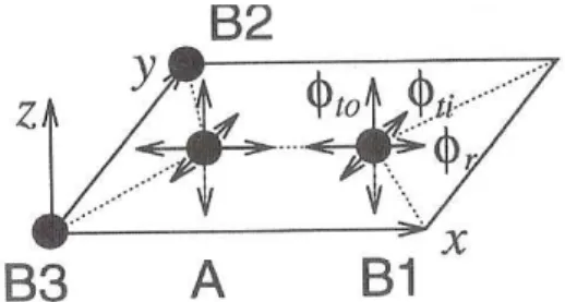
The remaining problem is to construct the force constant tensorK(i j). First we consider the force constant between an Aatom and a nearest-neighbor B1atom, both of them lying on the x-axis as shown in Fig. 1.9.

Figure 1.9: Force constants between theAandB1atoms on a graphene sheet. The interaction is

repre-sented by the components of the force constant tensorφr,φti andφtofor the nearest-neighbor atoms in

the radial (bond-streching), in-plane, and out-of plane tangential (bond-bending) directions, respectively.

B2andB3are the nearest neighbors equivalent toB1, whose force constant tensor is obtained by rotation

of the system. Figure taken from [20].

For the coordinate system defined in Fig. 1.9, the force constant tensor can be written in a diagonal form as

KAB1 ₌

             

φ(1)r 0 0

0 φ(1)_ti 0

0 0 φ(1)_to,

             

(1.56)

where φ(n)_r , φti,andφto represent the force constant parameters in the radial (bond-straching), in-plane and out-of-plane tangential (bond-bending) directions of thenth_{nearest neighbors,} re-spectively [20]. The graphene plane is in thexyplane, and the radial direction corresponds to the direction of theσ bonds. The two tangential directions (yandz) are taken to be perpendicular

to the radial direction. The corresponding phase factor exp (i~_k_·_∆_{Ri j}~ _{) becomes exp(}₋_{i kxa}_/√₃₎

for theB1atom at (a/√3,0,0).

(38)

KA,Bα ₌ _U−1

α KA

,B1_U_, (_α₌ 2_,3) (1.57)

where the unitary matrix U_α is here defined as a rotation matrix around the_z axis in Fig. 1.9, taking theB1atom into theBαatom,

U_α =

             

cosθα sinθα 0

−sinθα cosθα 0

0 0 1,

              (1.58)

As an example, the force constant matrix for theB2atom at (−a/(2√3),a/2,0), withU2 evalu-ated atθ₂= 2π/3, is given by

KAB2 ₌ 1

4              

φ(1)r +3φ(1)ti

√

3φ(1)_ti ₋φ(1)r

0

√

3φ(1)_ti ₋φ(1)r

3φ(1)r +φ(1)_ti 0

0 0 φ(1)_to

              , (1.59)

and the corresponding phase factor is exp(₋ikxa/(2

√

3)+ikya/2).

To calculate the phonon dispersion relations for graphene, the interaction between two nearest-neighbor atoms is not sufficient to reproduce the experimental results, and we generally need to consider contributions from long-distance forces, such as from thenth_{neighbor atoms, (n} ₌ 1,2,3,4, ...) [20]. The values for the force constantsφn_[₂₆_{] are obtained by fitting experimental} data over the Brillouin zone, as for example from inelastic neutron scattering or electron energy loss spectroscopy measurements along theΓMdirection [26,27].

Table 1.1: Force constants parameters for graphene obtained experimentally in units of 104 dyn/cm [26]. The subscripts r,ti, andtorefer to radial, transverse in-plane and transverse out-of-plane, respectively.

Radial Tangential

φ(1)r = 36.50 φ(1)_ti = 24.50 φ(1)to =9.82

φ(2)_r =8.80 φ(2)_ti =₋3.23φ(2)_to =₋0.40 φ(3)r =3.00 φ(3)ti =−5.25 φ

(3)

to =0.15

(39)

In Fig. 1.10 the phonon dispersion curves for graphene are shown using the set of force con-stants depicted in Table 1.1. The three phonon branches with null frequency at the Γpoint of the Brillouin zone correspond to the three acoustic modes, namely the out of plane, the in-plane tangential (bond-bending), and the in-plane radial modes listed in order of increasing energy, along theΓMofΓK directions. The remaining three branches correspond to the optical modes, one out of plane and two in plane.

Figure 1.10: Phonon dispersion in graphene along the high-symmetry directions in the Brillouin zone. Figure taken from [28].

Thus far, everything we did lies within the scope of classical mechanics. However an accu-rate description of the motion of the lattice requires quantum mechanical considerations. For instance there is a quantum mechanical analog for the classical lattice wave described by Eq. 1.43, and it is called aphonon. As expected, the energy carried by this excitation is quantized, as a single phonon of angular frequencyωcarries energy~_ω[29].

1.4 The electron-phonon interaction

(40)

1.4.1 The residual electric field

The best way to picture the origin of the electron-phonon interaction is to start by considering a vibration of a lattice of unscreened ions. We then allow the electron gas to flow into the re-gions of compression in order to restore the electrical neutrality of the system on a macroscopic scale. However, an increase in the local density of electrons must be balanced by extra kinetic energy according to the uncertainty principle. Therefore, these regions exhibit a lower electric potential energy and a higher kinetic energy for the electrons. The opposite is true for regions of decompression, where the decrease in the local density of electrons is balanced by a decrease in the kinetic energy resulting in a higher electric potential energy and lower kinetic energy for the electrons. In a more careful treatment, the electron gas would not completely screen the electric field of the ions, and they would not be able to restore the electrical neutrality of the system. Instead, the electrons would flow until the sum of the electric potential energy and the kinetic energy became uniform. There would then be a residual electric field tending to restore the ions to their equilibrium positions. The action of this residual electric field on the electrons that gives rise to the electron-phonon interaction [29].

1.4.2 The Fr¨ohlich Hamiltonian

The interaction of phonons with electrons is a complicated subject and the more complex the system is, the more difficult its mathematical treatment will be. In order to illustrate the main consequences of the interaction between phonons and electrons, in this section we shall consider our system to be a simple metal in which, the ions interact with each other and with the electrons only through a short-range screened potential. By making use of the second-quantized notation, the unperturbed Hamiltonian of our material system is

H₀₌ X

~_k

E_~

kc~†_kc~k +

X

~

q,~s

~ω~q,~sa_q_~†_,~_sa~q,~s (1.60)

withc_~† k anda

†

~

q,~s (c~k anda~q,~s) being the creation (annihilation) operators creating (annihilating) an electron in the state characterized by the wave vector~_{k, and a phonon with wave vector}_~_q

(41)

approximation.In this scenario, the perturbative Hamiltonian assumes the form

H_I ₌ X

~_k_,~_k′_,_l

h~k_|V(~r₋(~l+y~l))|~k ′

ic†_~ kc~k′

= X

~_k_,~_k′_,_l

ei(~k′−~k)·(~l+y~l)_V

~

k−~k′c

†

~_kc~k′

V~_k₋~_k′ = 1 Ω

Z

ei(~k′−~k)·~rV(~r)d~r

(1.61)

with Ω being the volume of the solid,~l and y~l the equilibrium position and the displacement from the equilibrium position of the ion, respectively. HereV(~r) is the potential due to a single

ion at the origin. Note that we are adopting plane wave expi(~_k_·_~_{r) solutions as the eigenstates}

of the unperturbed electrons. With the assumption that the displacementy~l of the ion (whose equilibrium position is~_{l) is sufficiently small to lead (}~_k₋~_k′₎

·y~l ≪1, we can write

ei(~k′−~k)·y~l _≃ 1₊i(~_k₋~_k′)_·_y_~

l =1+iN−1/2(~k₋~k′)_·X

~

q

ei~q·~ly~q. (1.62)

Where we used that

~

yl = N−1/2X

~q

ei~q·~lyq~. (1.63)

Here, Eq. 1.63 is the quantum analog of Eq. 1.43 and arises when solving the motion of the lattice in a quantum mechanical approach. Notice that, unlike Eq. 1.43, there is no time dependent term in this equation, which resembles a static wave solution. This is the underlying assumption behind the adiabatic Born-Oppenheimer approximation (ABO) which, as we shall see in Sec. 3.2.2, does not hold for graphene. However, we are going to use ABO to get some important results that will enable a better understanding of the electron-phonon interaction. Back to our analysis,the perturbative HamiltoninanH_I can be split in two parts,

H_I =H_Bloch+H_ep_, (1.64) with H_Bloch being the periodic potential of the stationary lattice, which is independent of the lattice displacements, and H_ep the electron-phonon interaction Hamiltonian.. For H_Bloch we have

H_Bloch ₌ X

~_k_,~_k′_,~_l

ei(~k′−~k)·l~V~_k₋~_k′c†_~

(42)

Now recall that a summation on the formP

~_lexpi(~q·~l) vanishes unless~qis equal to some~g, a

vector of the reciprocal lattice, in which case the sum is equal toN, the total number of atoms. Thus

X

~_k_,~_k′_,~_l

ei(~k′−~k)·~l = X

~_k_,~_k′_,~_l

δ~_k′₋~_k_,~_gei( ~_k′

−~k)·~l ₌_N

H_Bloch₌ _NX

~_k_,~_g

V₋~gc_~† k−~gc~k.

(1.66)

The electron-phonon Hamiltonian is given as

H_ep =iN−1/2 X

~

k,~k′,~l,~q

ei(~k′−~k+~q)·~l(~k′₋~k)_·~y~qV~_k₋~_k′c_~† kc~k′

=iN1/2X

~

k,~k′ (~_k′

−~k)·~y~_k₋~_k′V~_k₋~_k′c†_~ kc~k′.

(1.67)

Again, we made use of the property of summation over~_{l: it vanishes unless}~_k′

−~k+~q=~g.

Next, we express~y~_k₋~_k′ in terms of the creation and annihilation operators, a result that comes from the quantum treatment of the motion of the crystal:

~y~q=

~ 2Mω~_k₋~_k′_,~_s

!1/2

~sa†

−~q,~s+a~q,~s

(1.68)

Inserting Eq. 1.68 into Eq. 1.67 we get the expression for the Electron-Phonon interaction Hamiltonian,

H_ep = iX

~_k_,~_k′_,~_s

N~ 2Mω~_k₋~_k′_,~_s

!1/2 (~_k′

−~k)·~s V~_k₋~_k′(a_~†

k′−~k,~s+a~k−~k′,~s)c

†

~_kc~k′. (1.69)

For the sake of simplicity we shall assume the phonon spectrum to be isotropic, that is, the phonons will be either longitudinally or transversely polarized. With this assumption only the longitudinal modes, for which~sis parallel to~k′₋~k, are considered inH_ep. We shall also neglect the effects ofH_Bloch. After this simplifications we are left with the Fr¨ohlich Hamiltonian,

H = X

~_k

E_~ kc

†

~_kc~k +

X

~

q

~_ω_~_q_a†

~

qa~q+

X

~_k,~k′ M~_k~_k′

a†

−~q+a~q

c_~†

kc~k′, (1.70) where the electron-phonon matrix element is defined as

M~_k~_k′ =i N~ 2Mω~q

!1/2

~k

′

−~k

(43)

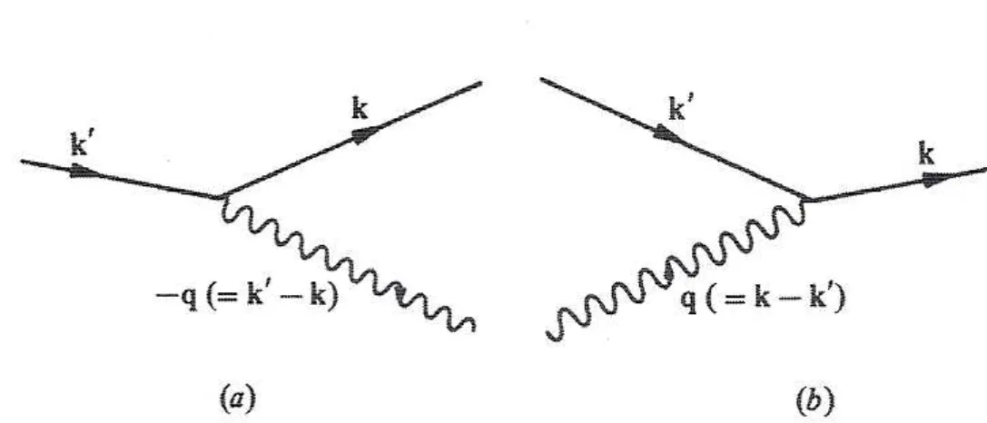
Figure 1.11: Diagrams representing the interaction terms in the Frohlich Hamiltonian. The electron is scattered from state~_k′

to state~_k_{either by (a) emission of (b) absorption of a phonon.}

Figure from [29].

with the phonon wavenumber~q, reduced to the first Brillouin zone, equals to~k₋~k′.

We can think of the electron-phonon HamiltonianH_ep as composed of two parts, terms involv-inga†₋_~_qc†_~

kc~k′ and terms involvinga

†

~

qc

†

~

kc~k′. These may be represented by the diagrams shown in Figs. 1.11(a) and1.11(b), respectively. In the first diagram we have an electron scattered from state~_k′

to state~_k_{by emission of a phonon with wavenumber}~_k′

−~k. In the second diagram the

electron is scattered from state~_k′

to state~_k _{by absorption of a phonon of wavenumber}~_k₋~_k′ [29].

1.4.3 Renormalization of the phonon frequencies and the Khon Anomaly

In order to determine how the electron-phonon interaction affects the phonon spectrum, we must use Perturbation Theory to calculate the energy of the system described by the Fr¨ohlich Hamiltonian. The first two terms of the Fr¨ohlich Hamiltonian1.70 are the unperturbed terms, while theH_ep term represents the perturbation. The energy up to second order inH_epis

|φ_ieither to create or destroy one phonon, the resulting wavefunction must be orthogonal to_|φ_i,

(44)

E₂ =_hφ_|X

~

k,~k′ M~_k~_k′

a†

−~q+a~q

c_~† kc~k′(

E₀₋H₀)−1

× X

~_k′′_,~_k′′′ M~_k′′~_k′′′

a†

−~q′ +a~q′

c†_~

k′′c~k′′′|φi

=_hφ_| X

~_k_,~_k′_,~_k′′_,~_k′′′

M~_k~_k′M~_k′′~_k′′′

h

a†

−~qc

†

~_kc~k′(E0−H0)− 1₊_a

~

qc_~† kc~k′(

E₀₋H₀)−1i

a₋~q′c†_k~′′c~k′′′ +a

†

~

q′c

†

~

k′′c~k ′′′

|φ_i.

(1.73)

By developing this expression, we have

E₂ ₌ X

~_k_,~_k′_,~_k′′_,~_k′′′

M~_k~_k′M~_k′′~_k′′′hφ|

a†

−~qc

†

~_kc~k′(E0−H0)− 1

a†

−~q′c

†

~

k′′c~k ′′′ + a†₋_~_qc_~†

kc~k′(

E₀₋H₀)−1_a_~

q′c†_k~′′c~k′′′ + a~qc_k†~c~k′(E0−H0)− 1

a†

−~q′c

†

~

k′′c~k′′′ + a~qc_~†

kc~k′(

E₀₋H₀)−1_a_~ q′c†_k~′′c~k′′′

|φ_i

(1.74)

The first and the fourth term inside the parenthesis in Eq. 1.74 vanish because the creation (annihilation) operators act twice on_|φ_iresulting in a wavefunction orthogonal to_|φ_i. Besides,

the second and third terms will vanish unless~_k′′′ _{is equal to}_~_{k, and}_~

k′′ is equal to~k′. Thus the contribution from the second order term is

E₂= _hφ_|X

~

k,~k′

M~_k~_k′

2h

a†

−~qc

†

~_kc~k′(E0−H0)

−1_a

−~qc†_~ k′c~k +a~qc_~†_kc~_k′(E₀−H₀)−1a†_~

qc

†

~

k′c~k|φi,

(1.75)

where we used M~_k′~_k = M~_k~_k′∗. The first term in brackets in Eq. 1.75 can be represented as in Fig. 1.12 (a). An electron is first scattered from the state~_k _to~_k′

with the absorption of a phonon of wavenumber₋~q=~k′₋~k. The factor (E₀₋H₀)−1then measures the amount of time the electron is allowed to stay in the intermediate state~_k′ _{by the Uncertainty Principle. In the} situation illustrated in Fig. 1.12 (a), the energy difference between the initial and intermediate states isE_~

k +~ω−~q −E~k′, so a factor of (E~k+~ω−~q−E~k′)−

1_{is considered. The electron is then} scattered back into its original state~_k_{with the re-emission of a phonon. The second term in Eq.}

1.75can be represented by Fig.1.12(b). An electron is first scattered from state~_k_{to state}~_k′ by emission of a phonon of wavenumber~q=~k₋~k′. In this case a factor of (E_~

k−(~ω~q+E~k′))− 1_is attained.