A (semi-)parametric functional coefficient autoregressive conditional duration model

Working

Paper

343

A (semi-)parametric functional

coefficient autoregressive

conditional duration model

Marcelo Fernandes

Marcelo C. Medeiros

Alvaro Veiga

CEQEF - Nº11

W_ORKING P_{APER 343}–CEQEF Nº 11•DEZEMBRO DE 2013• 1

Os artigos dos Textos para Discussão da Escola de Economia de São Paulo da Fundação Getulio Vargas são de inteira responsabilidade dos autores e não refletem necessariamente a opinião da

FGV-EESP. É permitida a reprodução total ou parcial dos artigos, desde que creditada a fonte.

Escola de Economia de São Paulo da Fundação Getulio Vargas FGV-EESP

A (SEMI-)PARAMETRIC FUNCTIONAL COEFFICIENT AUTOREGRESSIVE CONDITIONAL DURATION MODEL

Marcelo Fernandes

Sao Paulo School of Economics – FGV

School of Economics and Finance, Queen Mary University of London E-mail:marcelo.fernandes@fgv.br

Marcelo C. Medeiros

Department of Economics, Pontifical Catholic University of Rio de Janeiro E-mail:mcm@econ.puc-rio.br

Alvaro Veiga

Department of Electrical Engineering, Pontifical Catholic University of Rio de Janeiro E-mail:alvf@ele.puc-rio.br

ABSTRACT: In this paper, we propose a class of ACD-type models that accommodates overdispersion, intermittent dynamics, multiple regimes, and sign and size asymme-tries in financial durations. In particular, our functional coefficient autoregressive con-ditional duration (FC-ACD) model relies on a smooth-transition autoregressive speci-fication. The motivation lies on the fact that the latter yields a universal approximation if one lets the number of regimes grows without bound. After establishing that the suf-ficient conditions for strict stationarity do not exclude explosive regimes, we address model identifiability as well as the existence, consistency, and asymptotic normality of the quasi-maximum likelihood (QML) estimator for the FC-ACD model with a fixed number of regimes. In addition, we also discuss how to consistently estimate using a sieve approach a semiparametric variant of the FC-ACD model that takes the number of regimes to infinity. An empirical illustration indicates that our functional coefficient model is flexible enough to model IBM price durations.

KEYWORDS: explosive regimes, neural networks, quasi-maximum likelihood, sieve

estimation, smooth transition, stationarity.

ACKNOWLEDGEMENTS: We are grateful to Valentina Corradi, Emmanuel Guerre, Oliver Linton, Jos´e

Ant´onio Ferreira Machado, Olivier Scaillet, and Howell Tong for helpful discussions as well as to seminar

participants at Queen Mary, SoFiE European Conference (Geneva, Switzerland), Encontro Brasileiro

de Econometria (Natal, Brazil), 50 Years of the Econometric Institute (Rotterdam, The Netherlands),

Nonlinear Dynamical Methods and Time Series Analysis (Udine, Italy), and Econometrics in Rio (Rio

de Janeiro, Brazil) for valuable comments. We also thank Duda Mendes for able research assistance as

well as CNPq and Pronex/FAPERJ for financial support. The usual disclaimer applies.

1. INTRODUCTION

There has recently been a great interest in the implications of price durations in

em-pirical finance. Most emem-pirical analyses use one of the several extensions of Engle and

Russell’s (1998) linear autoregressive conditional duration (ACD) model that abound

in the literature. Fernandes and Grammig (2006) consider a family of ACD-type

mod-els that relies on asymmetric responses to shocks and on a Box-Cox transformation to

the conditional duration process. Their family encompasses most ACD-type models

in the literature, though there are a few exceptions. Zhang, Russell and Tsay (2001)

argue for a nonlinear version based on self-exciting threshold ACD processes, whereas

Meitz and Ter¨asvirta (2006) propose the smooth transition and the time-varying ACD

models. This paper puts forward a novel class of ACD-type models based on logistic

smooth-transition autoregressive processes with multiple regimes. In particular, our

functional coefficient autoregressive conditional duration (FC-ACD) model not only

nests the ACD-type processes proposed by Meitz and Ter¨asvirta (2006), but may also

serve as the basis for a semiparametric approach if one lets the number of regimes to

grow without bounds.

We first address the theoretical aspects of the FC-ACD process with a fixed number

of regimes. In particular, we establish sufficient conditions for strict stationarity and

for the existence of higher-order moments. It turns out that the conditions are quite

mild in that they do not exclude duration processes with explosive regimes. As in

Medeiros and Veiga (2009), we show that explosive regimes may entail very interesting

dynamics. In particular, strictly stationary FC-ACD processes with explosive regimes

are particularly suitable to model intermittent dynamics: The system spends a large

fraction of time in a bounded region, but sporadically develops an instability that grows

We then move to establishing sufficient conditions for model identifiability as well

as for the existence, consistency, and asymptotic normality of the quasi-maximum

like-lihood (QML) estimator. We derive consistency and asymptotic normality under

first-and second-order moment conditions, respectively. Finally, we develop a sequence of

simple Lagrange multiplier (LM) tests to determine the number of limiting regimes.

Although we derive the tests using the exponential distribution as reference, we also

discuss a robust version so as to cope with non-exponential errors.

We also consider a semiparametric version of the FC-ACD model in which the

number of extra regimesM increases with the sample size. The motivation rests on

the fact that the logistic smooth transition autoregressive process withM → ∞acts

as a universal neural-network approximation (Hornik, Stinchcombe and White, 1989).

The resulting semiparametric model encompasses most first-order ACD-type models

in the literature, despite the fact we impose some restrictions on the functional

coef-ficients specification to achieve identification of the nonparametric term as well as to

ensure stationarity and geometric ergodicity. To estimate the semiparametric model,

we rely on a regularization procedure that penalizes the log-likelihood function as one

increases the number of regimes. In particular, we employ Chen and Shen’s (1998)

results to provide asymptotic justification for the resulting sieve estimator.

We thus deem that we contribute to the literature in several aspects. First, in

con-trast to Meitz and Ter¨asvirta’s (2006) smooth transition ACD framework, our FC-ACD

specification permits modeling more than two limiting regimes as well as explosive

regimes. Second, our framework allows for statistical inference as to what concerns

the number of regimes, and hence it is not necessary to impose a priori a certain

num-ber of regimes as in Zhang et al. (2001). Third, we also consider the case in which

the number of regimes to increase with the sample size, so as to obtain a sieve

approx-imation for the conditional duration process. Finally, we demonstrate the practical

usefulness of the FC-ACD specification by modeling IBM price durations. The main

motivation lies on the fact that early findings clearly reject many of the extant

ACD-type specifications in the literature (see Fernandes and Grammig, 2006). We show that

allowing for multiple regimes facilitates substantially the task of reaching a congruent

specification for the IBM price durations.

The remainder of the paper is organized as follows. Section 2 outlines the

statisti-cal properties of the FC-ACD process, whereas Section 3 deals with quasi-maximum

likelihood estimation for a known fixed number of regimes. Section 4 then proposes

a sequential testing procedure to determine the unknown number of regimes. Section

5 next considers a semiparametric version of the FC-ACD model by letting the

num-ber of regimes increase with the sample size. Section 6 collects the findings of the

empirical application that we carry out aiming to model IBM price durations.

Sec-tion 7 summarizes the main results and offers some concluding remarks. We collect

all technical details concerning the derivations, including proofs and lemmas, in the

Appendix.

2. AFUNCTIONAL COEFFICIENTACDPROCESS

Let the durationxi=ti−ti−1denote the time spell between two events occurring at

timestiandti−1. For instance, we define price duration as the time interval necessary

to observe a cumulative change in the mid-price of at least some given value. To

account for the serial dependence that characterizes financial duration data, we assume

that durations follow an accelerated time failure process.

ASSUMPTION1. Letxi = ψiϵi. The sequence{ϵi;i ∈ Z}of iid random variables

has a continuous density functionf >0in[0,∞), withE(_ϵiFi−1)_{= 1, whereFi−1}

is the information set available at timeti−1. Also,ψi =E

( xi

_Fi−1

)

is independent of_{ϵi, ϵi+1, . . .}.

Assumption 1 is standard in the literature (see discussion in Drost and Werker,

conditional expected duration, viz. ψi = ω +α xi−1 +β ψi−1. Bauwens and Giot

(2000) propose a logarithmic version of the ACD model with a similar autoregressive

structure for the log rather than for the level of the expected duration so as to ensure

the positivity of the duration process. In this paper, we propose a more flexible model

based on a functional coefficient specification.

DEFINITION1. The durationxifollows a functional coefficient autoregressive

condi-tional duration (FC-ACD) process withM + 1regimes ifxi =ψiϵi, whereϵi andψi

satisfy Assumption 1 and

logψi =ω(logxi−1) +α(logxi−1) logxi−1+β(logxi−1) logψi−1 (1)

with

ω(logxi) = ω0+

M

∑

m=1

ωmGm(logxi) (2)

α(logxi) = α0+

M

∑

m=1

αmGm(logxi) (3)

β(logxi) = β0+

M

∑

m=1

βmGm(logxi), (4)

and

Gm(logxi) =G(logxi;γm, cm) =

1 1 + exp[−γm

(

logxi−cm

)]. (5)

The FC-ACD process belongs to the class of logistic smooth transition

autoregres-sive models. The parameter vector is

θ = (ω0, . . . , ωM, α0, . . . , αM, β0, . . . , βM, c1, . . . , cM, γ1, . . . , γM)′.

The slope parametersγm(m= 1, . . . , M) control the smoothness of the regime

transi-tions: e.g.,Gm(logxi)converges to a step function asγmgrows without bound.

Equa-tion (5) also implies that log-duraEqua-tions determine the weights at which each regime

contributes to the overall dynamics of the process at timeti. Alternatively, one may

resulting model thus is quite similar to Zhang et al.’s (2001) self-exciting threshold

ACD specification. The main differences are that we allow for smooth transitions and

that, as in Bauwens and Giot (2000), we model the log rather than the level of the

expected duration so as to avoid positivity constraints on the parameter space.

The FC-ACD specification entails several advantages. First, the condition we

de-rive in Subsection 2.1 for strict stationarity does not rule out the presence of explosive

regimes. The latter is interesting because it may give way to the moderately high,

but very persistent, autocorrelation structure that seems to characterize financial

dura-tion data. Second, our specificadura-tion nests the threshold ACD-type processes put forth

by Meitz and Ter¨asvirta (2006). Third, as in Medeiros and Veiga (2000), one may

interpret (2) to (4) as a single-hidden layer neural network withM hidden units. It

thus follows that the FC-ACD specification admits a semiparametric variant by letting

the number of regimes increase with the sample size. A neural network with a large

number of hidden units indeed approximates arbitrarily well any Borel-measurable

function (Hornik et al., 1989).

To establish the statistical properties of the FC-ACD process, we require a standard

regularity condition on the error term and on the parameter space.

ASSUMPTION2. The error termϵi is such thatE|logϵi|< ∞andE|ϵi|k <∞ for

some integerk≥4.

ASSUMPTION3. The vectorθis interior to the compact parameter spaceΘ⊆R5M+3_.

The asymptotic normality of the QML estimator depends heavily on the

fourth-moment requirement in Assumption 2. If the interest lies only on the consistency of

the QML estimator, then it suffices to assume that the finiteness of the second moment.

2.1. Statistical properties: Strict stationarity and geometric ergodicity. Letui =

transition probability in view that

ui+1=F(ui;θ) +εi+1, (6)

whereF(ui;θ) = [F(ui;θ),0]′with

F(ui;θ) =ω(logxi) + [α(logxi) +β(logxi)] logxi+α(logxi) logϵi,

andεi = [0,logϵi]′. We are now ready to establish our first theoretical result.

THEOREM 1. Suppose that the duration xi follows a FC-ACD process withM + 1

regimes satisfying Assumptions 1 and 2. IfA0 <1,AM <1, andA0AM <1, where

A0 =α0 +β0andAM =∑Mm=0(αm+βm), then strict stationarity and geometric

ergodicity hold for the duration process andE_|logxi|k_{<∞, withkas in Assumption}

2.

The sufficient condition in Theorem 1 is intuitive and simple despite not only the

highly nonlinear nature of the model but also the extant sufficient conditions in the

lit-erature (Meitz, 2006; Fernandes and Grammig, 2006; Meitz and Saikkonen, 2008). As

in threshold autoregressive models (Tong, 1990), it suffices to impose constraints only

on the two polar regimes. In particular, it allows strictly stationary and ergodic

FC-ACD processes to have explosive regimes. This is of particular interest given that such

processes are suitable to model intermittent dynamics (Medeiros and Veiga, 2009).

An ergodic FC-ACD process with explosive regimes indeed spends a large fraction

of time in a bounded region, though it sporadically develops an instability that grows

exponentially for some time and then suddenly collapses. As we illustrate in Example

1, even though we only consider first-order specifications, the FC-ACD process admits

a highly persistent behavior with moderate values for the autocorrelation function,

es-pecially in the presence of explosive regimes.

EXAMPLE 1. Consider a FC-ACD process with three limiting regimes, exponential errors, and parametersω0 = 0.005,ω1 = −0.9, ω2 = 3, α0 = 0.09, α1 = −0.05, α2 =−0.05,β0 = 0.9,β1 = 0.6,β2 =−0.5,γ1 = 1000,γ2 = 100,c1 =−2, and

0 1000 2000 3000 4000 5000 6000 7000 8000 9000 10000 0

0.05 0.1 0.15 0.2 0.25

event time

durations

0 20 40 60 80 100 120 140 160 180 200 −0.05

0 0.05 0.1 0.15 0.2 0.25 0.3

lag

sample autocorrelations

FIGURE1. Simulated path and autocorrelation function of a FC-ACD process with three limiting regimes, exponential errors, and parame-tersω0 = 0.005, ω1 = −0.9, ω2 = 3, α0 = 0.09, α1 = −0.05, α2 =−0.05,β0 = 0.9,β1 = 0.6,β2 =−0.5,γ1 = 1000,γ2 = 100, c1 =−2, andc2 = 1.

c2 = 1. The condition for strict stationarity holds given thatA0 = α0+β0 = 0.99, A2 = ∑2m=0(αm +βm) = 0.99 andA0A2 = 0.9801, despite the explosiveness of

the second regime. Figure 1 depicts a simulated path of such duration process and the corresponding autocorrelation function up to the 200th lag.

3. QUASI-MAXIMUM LIKELIHOOD ESTIMATION

In this section, we carefully address the parametric estimation of the FC-ACD

model. To avoid further distributional assumptions, we invoke quasi-maximum

identification as well as for the consistency and asymptotic normality of the QML

es-timator.

The derivation of the semiparametric ACD model in Drost and Werker (2004)

clar-ifies that adaptiveness occurs if and only if the error distribution belongs to the

two-parameter gamma family with unit mean. It actually turns out that the exponential

and gamma scores are proportional, and hence there is no efficiency loss in restricting

attention to the exponential distribution. This means that the QML estimator is

con-sistent only if we write the likelihood as if under the assumption of exponential (or

standard gamma) distribution (Bickel, 1982). The quasi-log-likelihood thus reads

LN(θ) =

1 N

N

∑

i=1

ℓi(θ), (7)

where

ℓi(θ) =−logψi−

xi

ψi

.

We treat the unobservable sequence_{(x−i, ψ−i) ;i∈N}as constant rather than

ran-dom. The quasi-log-likelihood is thus suitable for practical applications given that it is

not conditional on the true initial value(x0, ψ0).

To derive the asymptotic properties of the QML estimator, it is convenient to work

also with the unobserved process_{(xu,i, ψu,i) ;i∈Z}, which satisfies

xu,i = ψu,iϵu,i

logψu,i = ω0+α0 logxu,i−1+β0 logψu,i−1

+

M

∑

m=1 [

ωm+αm logxu,i−1+βm logψu,i−1 ]

Gm(logxi).

(8)

The unobserved quasi-log-likelihood conditional on_F0 = (x0, x−1, x−2, . . .)is

Lu,N(θ) =

1 N

N

∑

i=1

ℓu,i(θ), (9)

with ℓu,i(θ) = −logψu,i − x_ψu,i

u,i. As is apparent, the primary difference between

LN(θ)andLu,N(θ)is that the latter is conditional on an infinite series of past

based on (9). Let

b

θN = argmax

θ∈Θ L

N(θ) = argmax

θ∈Θ

1 N

N

∑

i=1

ℓi(θ), (10)

and

b

θu,N = argmax

θ∈Θ L

u,N(θ) = argmax

θ∈Θ

1 N

N

∑

i=1

ℓu,i(θ). (11)

Subsection 3.1 next discusses the existence of_L(θ) =E_[ℓu,i(θ)], so as to tackle the

identifiability of the FC-ACD model in Subsection 3.2. Subsection 3.3 then derives the

consistency and asymptotic normality of the QML estimators in (10) and (11) under

second- and fourth-order moment conditions, respectively.

3.1. Existence of the QML estimator. It is easy to appreciate that the QML

esti-mator exists only if _L(θ) = E_[ℓu,i(θ)]exists. The next result immediately follows

from White’s (1996) Theorem 2.12, which establishes that_L(θ)exists under certain

continuity and measurability conditions on the quasi-log-likelihood function.

THEOREM 2. If the duration xi follows a strictly stationary and ergodic FC-ACD

process withM+ 1regimes, then, for any parameter vectorθ _∈Θ,_L(θ)exists and is finite under Assumptions 1 and 3.

3.2. Identifiability of the model. A fundamental problem that usually haunts

nonlin-ear econometric models is the lack of identifiability of the empirical loss function. To

carry out statistical inference, we must first show thatθ0 is the unique maximizer of

L(θ). It turns out, however, that we achieve neither global nor local identification of

the FC-ACD model without imposing some parametric constraints.

There are three reasons for the model unidentifiability. First, as the multiple regimes

correspond to hidden units in neural networks, they are interchangeable. This means

that the empirical loss function of the FC-ACD specification is invariant to regime

permutations, and hence there are (M + 1)!equal local maxima for the

(2004) for a discussion. Second, the logistic function in (5) is such that

G(logxi;γm, cm) = 1−G(logxi;−γm, cm).

This property evidently compromises model identifiability. Third, identifiability also

relates to model reducibility as it automatically imposes constraints on the vector of

parametersθm = (ωm, αm, βm, γm, cm)′ that defines the extra regimes of the

FC-ACD model(m = 1, . . . , M). For instance, it is not possible to identify the logistic

parameters(γm, cm)if(ωm, αm, βm)′ = 0, whereas(ωm, αm, βm, cm)′may take on

any value without affecting the value of the quasi-log-likelihood function ifγm = 0.

We then restrict the parameter spaceΘso as to circumvent such problems.

ASSUMPTION4. The parameter spaceΘis such that any vectorθ_∈Θsatisfies

C1: c < c1 < . . . < cM <c¯for some finite constantscand¯c;

C2: γm>0form= 1, . . . , M and

C3: (ωm, αm, βm)̸=0for somem∈ {0, . . . , M}.

THEOREM 3. Assumptions 1 to 4 ensure the global identifiability of the FC-ACD model and thatL(θ)has a unique maximum atθ₀.

Despite the fact that Assumption 4 is not verifiable, one may alleviate the risk of

irrelevant regimes by carrying out a sequence of LM tests (see Section 4).

3.3. Asymptotic theory. Our interest lies on the large sample properties of the QML

estimator given by (10). To derive the next result, we first establish that the unfeasible

QML estimator in (11) converges in probability toθ0and then show that the difference

between the two QML estimators shrinks to zero as the sample sizeN grows without

bound.

THEOREM 4. Under Assumptions 1 to 4, the QML estimators in (10) and (11) are consistent, i.e.,bθu,N

p

→θ0andbθN p

To complete the asymptotic characterization of the QML estimator, we first

intro-duce some notation and then establish the asymptotic distribution of the QML

estima-tor. Let

A0=E [

− ∂ 2_ℓ

u,i(θ)

∂θ∂θ′

_θ 0 ]

B0 = 1 N N ∑ i=1 E (

∂ℓu,i(θ)

∂θ θ0

∂ℓu,i(θ)

∂θ′

θ0 )

and denote their empirical counterparts by

AN(θ) =

1 N N ∑ i=1 [

∂2_logψ

i

∂θ∂θ′

( 1₋ xi

ψi

) + xi

ψi

∂logψi

∂θ

∂logψi

∂θ′

]

BN(θ) =

1 N N ∑ i=1 ( xi

ψi −

1 )2

∂logψi

∂θ

∂logψi

∂θ′ .

We are now ready to state that the QML estimator weakly converges to a Gaussian

distribution with the usual asymptotic covariance matrix (White, 1982).

THEOREM5. Under the conditions we assume in Theorem 4, it follows that

√

N(bθN−θ0)→ Nd (0,A−01B0A−01 )

(12)

and thatAN(bθN)andBN(bθN)consistently estimateA0 andB0, respectively. 3.4. Optimization algorithm. As in any smooth-transition specification, the

likeli-hood function of the FC-ACD model is very likely flat, especially for the transition

parameters. This means that one must carry out the optimization in a very careful

fashion. That is why we initially employ a genetic algorithm based on a population of

500 sets of initial values for the parameters that meet the strict stationarity conditions

in Theorem 1. We then switch to the BFGS nonlinear-optimization algorithm using as

initial values the solution of the genetic-algorithm procedure.

4. DETERMINING THE NUMBER OF REGIMES

As the FC-ACD specification in Definition 1 depends on the unknown number of

a sequential procedure in which we start with a small model and then decide whether

it pays off to add more regimes using some model selection criterion. This typically

boils down to some sort of likelihood ratio testing, where the particular choice of the

model selection criterion determines the asymptotic significance level of the test (see

Ter¨asvirta and Mellin, 1986).

There is a serious drawback in such approach, however. Suppose the data

gener-ating mechanism is a FC-ACD process withM regimes. Applying a model selection

criterion to decide whether to considerM + 1regimes requires the estimation of an

unidentified model withM logistic functions. It thus is impossible to estimate the

pa-rameters in a consistent manner, so that numerical problems likely arise in the QML

estimation. Besides, the lack of identification under the alternative hypothesis ofM+1

regimes also contaminates the likelihood ratio statistic, which does not converge to the

usualχ2 _{distribution under the null hypothesis ofMregimes.}

We therefore take a different approach to determining the number of regimes of the

FC-ACD model. Although we keep relying on a specific-to-general modeling

strat-egy, we circumvent the identification problem using sequential LM-type tests. Our

sequential testing procedure controls for the significance level of the individual tests

using Bonferroni’s upper bound for the overall significance level. In what follows, we

discuss our framework assuming exponential errors and then show how to robustify

the procedure so as to cope with nonexponential errors.

Consider an ergodic FC-ACD process withM + 1 regimes as in (1)–(5). To test

whether it is necessary to include the term corresponding to the(M+ 1)th regime, viz.

(ωM +αMlogxi−1+βMlogψi−1)GM(logxi−1;γM, cM), (13)

we define the null and alternative hypotheses as H_{M:γM = 0}and H_{M+1: γM >0,}

respectively. To remedy the lack of identification of the FC-ACD model withM+ 1

regimes under the null, we expand the logistic function GM around γM = 0 as in

Meitz and Ter¨asvirta (2006).

A first-order Taylor expansion ofGM aroundγM = 0then yields

logψi= ˜ω0+ ˜α0logxi−1+ ˜β0logψi−1

+

M_∑−1

m=1

[ωm+αmlogxi−1+βmlogψi−1]Gm(logxi−1)

+δ1logψi−1logxi−1+δ2(logxi−1)2+O (

γ_M2 ),

(14)

whereω˜0 = ω0+ 1₂ωM − 1₄ωMγMcM,α˜0 = α0 + 1₂αM +₄1γM(ωM −αMcM),

˜

β0 =β0+1₂βM−1₄βMγMcM,δ1 = 1₄βMγM, andδ2 = 1₄αMγM. Under the null of

H_{M:γM = 0, the specification in (14) reduces to the FC-ACD model withM}regimes.

Before stating the next result, we first establish some notation. Letφ= [θ′

,δ′

]′ _with

δ = (δ1, δ2)′. The QML estimator ofφunder the null hypothesis of HM: γM = 0

isφb_N = [bθN,0]. Letψbi ≡ψi

( b

φ_N)denote the estimate of the expected conditional

duration under the null anddbi = ∂log_∂φψi

_φ

=φb_N correspond to the derivative oflogψi

with respect to φ evaluated at the QML estimatorφb_N. Althoughbdi is recursive in

that it depends ondbi−1, it is straightforward to calculate it as a function of the initial

valuex0 of the duration process as in Medeiros and Veiga (2009). We are now ready

to state the asymptotic distribution of the LM statistic to test H_{M: γM = 0}against

H_{M+1:γM >0.}

THEOREM 6. Let the duration xi follow a strictly stationary and ergodic FC-ACD

process withM regimes. Assumptions 1 to 4 ensure that

LM =N [_N

∑

i=1 (

xi

b ψi

−1 )

b

d′_i

] ( _N ∑

i=1 b

didb ′

i

)−1[ _N ∑

i=1 (

xi

b ψi

−1 )

b

di

]

(15)

has an asymptoticχ2₂distribution under the null of H_{M:γM = 0.}

To avoid the exponential assumption, one may consider a robust version of the LM

test that is suitable to nonexponential errors, as in Meitz and Ter¨asvirta (2006), using

the tools in Wooldridge (1990, Procedure 4.1). The three steps of the resulting robust

testing procedure are as follows.

(2) Regress _∂∂_θ logψi

φ=φbNon

∂ ∂δ logψi

φ=φbN and compute the vector of

resid-uals_brifori= 1, . . . , N.

(3) Regress 1 on(xi/ψbi−1

) b

riand compute the resulting sum of squared

resid-ualsSSR. The robust test statisticLMR =N −SSRhas an asymptoticχ2₂

distribution under the null hypothesis of H_M.

We now combine the above statistical ingredients into a coherent modeling strategy

that involves a sequence of robust LM tests. The idea is to test a FC-ACD model

with only one regime against an alternative model with two regimes at the significance

levelλ1. In the event we reject the null, we keep testing FC-ACD specifications with

Jregimes against alternative models withJ+ 1regimes at the significance levelλJ =

λ1C1−J for some arbitrary constantC >1. We terminate the testing sequence at the

first nonrejection outcome and then estimate the number of extra regimesM of the

FC-ACD specification byMc = ¯J ₋1, whereJ¯refers to how many testing runs are

necessary to lead to the first nonrejection result. By reducing the significance level

at each step of the sequence, we are able to control the overall significance level and

hence to avoid excessively large models. The Bonferroni procedure indeed ensures

that such sequence of robust LM tests is consistent and that∑J_J¯₌₁λJ acts as an upper

bound for the overall significance level. As for the selection of the arbitrary constant

C, it is good practice to carry out the sequential testing procedure with different values

ofCso as to avoid models that are too parsimonious.

5. ASEMIPARAMETRIC VARIANT

In this section, we take benefit from the fact that the logistic smooth transition

autoregressive specification in (2) to (4) corresponds to a single-hidden layer neural

network with M hidden units. This implies that, if M is large enough, it

approxi-mates arbitrarily well any Borel-measurable function (Hornik et al., 1989; Chen and

White, 1998). We therefore consider a semiparametric version of the FC-ACD model

the dependence on the sample size, we denote the number of extra regimes byMN in

this section.

DEFINITION 2. The durationxi follows a semiparametric FC-ACD process if xi =

ψiϵi, whereϵiandψisatisfy Assumption 1 withσ2ϵ =Elogϵ2i ≤ ∞and

logψi =ω(logxi−1) +β logψi−1 (16)

with _|β_| < 1 and ω(_·) < _∞ belonging to the functional space _H of continuous bounded functions with finite first absolute moments of the Fourier magnitude dis-tributions.

This definition complements well Drost and Werker’s (2004) semiparametric

ap-proach, whose focus is on the error distribution rather than on the specification of the

conditional expected duration. It indeed encompasses most first-order ACD-type

mod-els in the literature, despite the fact that we impose three restrictions on the functional

coefficients specification. First, we confine attention to duration processes that satisfy

strict stationarity with finite second moments, geometric ergodicity, andβ₋mixingness

with exponential decay by assuming thatω(_·)is bounded and that_|β_|<1(see Meitz

and Saikkonen, 2008). This ensure that we may apply Chen and Shen’s (1998)

asymp-totic theory for sieve extremum estimates under weak dependence.

Second, we eliminate the slope functional coefficient in (1) — i.e., α(z)z — to

achieve identification of the nonparametric component in (16). Third, we restrict the

recursiveness of the conditional expected duration process by assuming thatβis

con-stant across regimes. This simplifies matters a lot for it permits rewriting the

semipara-metric FC-ACD model as a tractable nonlinear AR model of infinite order, namely,

logxi = ω(logxi−1) +β logψi−1+ logϵi

=

∞

∑

j=0

As the largeness of the functional space _H may compromise the estimation, we

approximate _H with a sequence _HN of sieve spaces (Grenander, 1981; Chen and

Shen, 1998) that becomes dense in_Has the sample size increases. As the sieve spaces

correspond to finite-dimensional parameter spaces, they only require parametric

esti-mation. In particular, we approximate the functionω_{∈ H}withωN ∈ HN, where

ωN(·) =ω₀(N)+ MN

∑

m=1

ω_m(N)G(_mN)(_·) (18)

andG(mN)(·) is the logistic function in (5) with finite parameterscm(N) andγm(N). We

restrict the parameter space so that∑MN

m=0|ω (N)

m | ≤ c,|c(mN)| ≤ c, and|γm(N)| ≤ cfor

some generic constantc < ∞. Makovoz (1996) demonstrates that the approximation

error is such that_∥ωN−ω∥=O

( M−1

N

)

, where_{∥· ∥}denotes theL2norm.

The resulting vector of parameters then is

θ₍N)= (

ω(₀N), . . . , ω(_MN)

N, c

(N) 1 , . . . , c

(N)

MN, γ

(N) 1 , . . . , γ

(N)

MN, β

) .

Instead of alluding to the sequence_HN of sieve functional spaces, we sometimes refer

to the corresponding sequenceΘ_(N)of sieve parameter spaces so as to emphasize the

parametric nature of the estimation problem. In accordance with the sieve literature,

we then approximate the first term of the right-hand side of (17) by

logψ_i(N)=

JN

∑

j=0

βjωN(logxi−1−j). (19)

This means that we actually employ two sieve approximations. The first truncates

the infinite summation in (17) by means of JN, whereas the second relates to the

finite number of extra regimesMN in the neural network. The next result documents

the conditions under which our semiparametric approach is consistent. The proof is

straightforward, relying on the fact that (19) converges to the first term of the

right-hand side of (17) as bothJN andMN go to infinity with the sample size.

THEOREM7. If the duration processxisatisfies Definition 2, the sieve approximation

error is negligible as long asJN → ∞andM_N3 logMN =O(N).

To avoid overfitting, we take a regularization approach by penalizing the empirical

loss function so as to control for the number of extra regimesMN (i.e., the number of

hidden units in the neural-network approximation) as well as for the number of lags

JN in the nonlinear AR representation. Let

LN(θ(N)) = 1 N

N

∑

i=1

ℓ(_iN)(θ₍N) )

, (20)

where

ℓ(_iN)(θ_(N))=−logψ_i(N)− xi

ψ_i(N) +λN

θ_(N),

λN is a regularization factor that shrinks to zero as the sample size increases. The

sieve estimator then is

b

θ_(N)= argmax

θ(N)∈Θ(N)

1 N

N

∑

i=1

ℓ(_iN)(θ_(N)). (21)

Given that_L(θ_(N)) = E

[

ℓ(_iN)(θ_(N))]is uniquely identified, the sieve estimator in

(21) is well defined and hence Chen and Shen’s (1998) results hold.

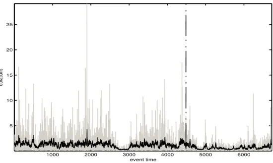
6. REVISITINGIBMPRICE DURATIONS

In this section, we estimate the FC-ACD model for the price durations of the IBM

stock traded on the New York Stock Exchange (NYSE) from September to November

1996. In contrast to Zhang et al.’s (2001) empirical analysis of IBM durations, we

do not fix the number of regimes in that we let the data determine the proper number

of regimes using either a sequence of LM-type tests or a regularization approach in

the parametric and semiparametric contexts, respectively. We define price duration as

the time interval necessary to observe a cumulative change in the mid-price of at least

$0.125. The main interest in models for price durations is due to the fact that they

permit retrieving intraday estimates of the instantaneous volatility of the price process

(Engle and Russell, 1998).

Apart from the opening auction, NYSE trading is continuous from 9:30 to 16:00.

1000 2000 3000 4000 5000 6000 5

10 15 20 25

event time

price duration

50 100 150 200 −0.05

0 0.05 0.1 0.15 0.2

lag

sample ACF

1 2 3 4 5 6

x 104 5

10 15 20

event time

trade duration

50 100 150 200 −0.05

0 0.05 0.1 0.15 0.2

lag

sample ACF

FIGURE 2. The first plot displays the time series of IBM price du-rations from September to November 1996, whereas the second plot exhibits its sample autocorrelation function up to 200 lags. The data correspond to diurnally adjusted durationsxi = Di/ϱ(ti), whereDi

is the plain duration in seconds andϱ(·)denotes the diurnal factor de-termined by first averaging the durations over thirty minutes intervals for each day of the week and then fitting a cubic spline with nodes at each half hour.

the NYSE as well as overnight spells. It is well known that financial durations feature

a strong time-of-the-day effect. We therefore consider diurnally adjusted durations

xi = Di/ϱ(ti), where Di is the plain price duration in seconds andϱ(·)denotes the

diurnal factor determined by first averaging the durations over thirty minutes intervals

for each day of the week and then fitting a cubic spline with nodes at each half hour.

The resulting (diurnally adjusted) durations serve as input for the remainder of the

analysis.

A comparison between price and trade durations mirrors the fact that the IBM stock

seconds and it takes several transactions to alter the mid-quote price by at least $0.125.

The sample size indeed reduces from 60,454 to 6,728 observations once we filter the

data to compute price durations. Table 1 describes the main statistical properties of the

IBM price durations. We compute descriptive statistics for both plain and diurnally

adjusted data for two subsamples. We employ the first subsample with 4,484

observa-tions for estimation purposes, reserving the second subsample with 2,244 observaobserva-tions

for out-of-sample analysis.

The distributions of the price durations in the first and second subsamples are

sub-stantially different, regardless of the time-of-the-day adjustment. For instance, if one

restricts attention to the diurnally adjusted series, the first-subsample mean, standard

deviation, first quartile, and median are about twofold their counterparts in the second

subsample. In addition, the third quartile declines by more than one half from the first

to the second subsample, whereas the maximum value in the first subsample is

three-fold the maximum in the second subsample. The minimum value and overdispersion

are the only statistics that remain approximately constant across subsamples.

The evidence in favor of overdispersion is also robust to the time-of-the-day

ef-fect. The latter feature ensures that it is not an artifact due to data seasonality. Figure

2 displays the diurnally adjusted series of IBM price durations as well as its

sam-ple autocorrelation function up to 200 lags. It reveals that IBM price durations are

very persistent in that there are significant positive values in the sample

autocorrela-tion funcautocorrela-tion at very high orders. Altogether, the combinaautocorrela-tion of overdispersion and

persistent autocorrelation in IBM price durations warrants the estimation of FC-ACD

models with multiple regimes.

We then estimate by quasi-maximum likelihood the FC-ACD model of first order

using the exponential distribution as reference. Table 2 reports the estimation and

testing results for models with one and two regimes given that our modeling cycle

−6 −5 −4 −3 −2 −1 0 1 2 3 4 0

0.1 0.2 0.3 0.4 0.5 0.6 0.7 0.8 0.9 1

log(x_i−1)

logistic transition function

FIGURE 3. The graph plots the logistic function in (5) against the sample values of the transition variable for c1 = 0.3210 and γ = 496.99. The transition variable is the past value of the logarithm of the diurnally adjusted IBM price duration, whereas the sample consists of the first 4,484 observations from the period ranging from September to November 1996.

LM test for additional regimes indeed does not reject the null of only two limiting

regimes at the usual levels of significance. Although the transition between the two

regimes is very abrupt given the large value ofγˆ1, Figure 3 shows that there are enough

observations (i.e., about 200 data points) within the transition phase to estimate the

parameters of the logistic function with reasonable precision.

The first regime is extremely persistent, withAˆ0 = ˆα0 + ˆβ0 = 0.9909, whereas

persistence subsides in the second regime given that Aˆ1 = ˆα0 + ˆα1 + ˆβ0 + ˆβ1 =

0.8696. The less persistent second regime mostly affects larger durations in view that

exp(ˆc1) = 1.3784lies slightly above the sample mean of the IBM price durations, at

the 78% percentile. This is somewhat in line with the evidence put forth by Zhang et

al. (2001), though they assume nonsmooth transitions between three fixed (rather than

1000 2000 3000 4000 5000 6000 5

10 15 20 25

event time

durations

FIGURE 4. The plot displays the actual and fitted values of the IBM price durations from September to November 1996. Actual values are in gray, corresponding to diurnally adjusted IBM price durations. Fitted values are in black, relating to the estimates of the expected duration of the FC-ACD model with two regimes for the parameter values in Table 1. The dashed vertical line marks the sample splitting for estimation and forecasting purposes.

The results for the FC-ACD model with one regime, which corresponds to Bauwens

and Giot’s (2000) logarithmic ACD model, show that ignoring the second regime

af-fects substantially the analysis of persistence. The persistence of the one-regime model

is a convex combination of the very distinct degrees of persistence that characterize the

first and second regimes of the FC-ACD model. In particular, it is closer to the

persis-tence in the first regime, which seems to prevail for 3,117 out of the 4,484 observations

of the in-sample period. Allowing for the second regime not only entails a better

pic-ture of the persistent napic-ture of IBM price durations, but also substantially improves

both the in-sample and out-of-sample fits as measured by the quasi-likelihood

func-tion values.

Figure 4 displays the actual and fitted values of the IBM price duration for the full

price durations, it is evident that it tracks well the movements in the latter series. The

in-sample and out-of-sample correlations between the actual and fitted log-values are

quite reasonable, namely, 0.3832 and 0.3069, respectively. They add up to an overall

correlation between actual and fitted log-values of 0.4391 in the full sample.

Fur-thermore, the in-sample and out-of-sample residuals of the FC-ACD model with two

regimes also have well-behaved distributions in that their mean and standard deviation

are close to unity (as expected given the exponential benchmark). The in-sample

resid-uals have a mean of 1.0001 with a standard deviation of 1.1536, whereas the mean and

standard deviation of the out-of-sample residuals are 0.8949 and 1.0152, respectively.

The overdispersion coefficients of the in-sample and out-of-sample residuals are

re-spectively 1.1536 and 1.1344, and hence well below the overdispersion that we report

in Table 1 for the IBM price durations.

To check for misspecification, we also inspect whether the in-sample and

out-of-sample residuals display any serial correlation by looking at the out-of-sample

autocorrela-tion funcautocorrela-tion up to 200 lags. Table 2 documents that the FC-ACD model with two

regimes does a much better job in accounting for the serial dependence in the IBM

price durations than Bauwens and Giot’s (2000) logarithmic ACD model. The

resid-ual autocorrelation reduces by a palpable amount as one allows for the second regime.

The decline is particularly strong for the in-sample residuals in that their maximum

autocorrelation (in magnitude) for the one-regime model is about twofold the one of

the FC-ACD model with two regimes.

7. CONCLUSION

This paper proposes a functional coefficient ACD model that accommodates

overdis-persion, intermittent dynamics, multiple regimes, as well as sign and size asymmetries

in financial durations. In particular, we rely on a very flexible smooth-transition

au-toregressive specification with multiple regimes. The motivation lies on the fact that

to infinity. We formally address how to consistently estimate the parametric FC-ACD

model with fixed number of regimes by quasi-maximum likelihood as well as the

semi-parametric counterpart using a sieve approach.

An empirical illustration indicates that our functional coefficient specification is

flexible enough to model IBM price durations in a congruent manner. This is in stark

contrast with the alternative model with a single regime, whose residuals display much

larger autocorrelations. In addition, we also evince that the FC-ACD model with two

regimes outperforms the one-regime model in goodness-of-fit terms both in-sample

APPENDIXA. PROOFS

Proof of Theorem 1. We start by casting the FC-ACD process with multiple regimes into a smooth transition autoregressive moving average (STARMA) representation. Letω¯i−1 ≡ ω(logxi−1), α¯i−1 ≡ α(logxi−1), and β¯i−1 ≡ β(logxi−1). It follows from (1) that the duration process has the following STARMA(1,1) representation:

logxi= ¯ωi−1+[α¯i−1+ ¯βi−1]logxi−1+ logεi−β¯i−1logεi−1. (A.1)

Following similar steps to Zhang et al. (2001), it is straightforward to show that the Markov chain in (6) is aϕ-irreducible T-chain. This means that we may apply Tweedie’s (1975) drift criterion to derive sufficient conditions for strict stationarity and geometric ergodicity. In ad-dition, Ling’s (1999) Theorem 4.1 implies that both strict stationarity and ergodicity of the functional coefficient ARMA model depends exclusively on its autoregressive part, and hence we confine attention to the analogous STAR(1) process withM+ 1regimes

yi= ¯νi−1+ ¯ζi−1yi−1+ςi, (A.2)

whereν¯i−1≡ν0+∑Mm=1νmGm(yi),ζ¯i−1≡ζ0+∑Mm=1ζmGm(yi−1), and the error term ςi is iid withE|ςi| < ∞. The sufficient conditions for strict stationarity that we derive are exactly the same for TAR(1) processes (see, e.g., Chen and Tsay, 1991), though our deriva-tion differs in view that (A.2) involves smooth transideriva-tions. For anyeC > 0, there exists a positive constantC > max_{|c_|,_|c¯_|}such thatζ¯i−1−ζ0

_≤ eC for anyyi−1 <−C and

ζ¯i−1−∑Mm=0ζm

≤eCfor anyyi−1> C. It then follows that

yi= ¯νi−1+1{yi−1<−C}

¯

ζi−1yi−1+1{|yi−1|≤C}

¯

ζi−1yi−1+1{yi−1>C}

¯

ζi−1yi−1+ςi,

where1Ais the indicator function that takes value one ifAis true and zero, otherwise. Taking absolute values of both sides gives way to

|yi| ≤ LC+1{yi−1<−C}

_ζ¯_{i−1|yi−1|+1{y}

i−1>C}

_ζ¯_{i−1|yi−1|+|ςi|}

≤ LC+ζi+−1|yi−1|+|ςi|

≤ |y0|∏ij−=01ζ +

j + i−1

∑

k=1

(|ςk|+LC)∏_ji−₌1_kζ_j++|ςi|+LC,

whereζ_i+_−1≡1{yi−1<−C}(|ζ0|+eC) +1{yi−1>C}

(

∑Mm=0ζm

+eC

)

andLCis a positive

constant that exceeds_|¯νi−1|+1{yi−1<−C}

_ζ¯_{i−1C. We then take conditional expectation} yielding

E(_|yi|y0) _{≤ |y0|}E( ∏i−1 j=0ζ

+

j

y0)+

i−1

∑

k=1

E[_(|ςk|+LC)∏i−1 j=kζ

+

j

y0]+E_|ςi|+LC

= _|y0_|E( ∏i−1 j=0ζ

+

j

y0)+L∗C

[

1 + i−1

∑

k=1

E( ∏i−1 j=kζ

whereL∗

C ≡E|ς1|+LC. We now have four cases to evaluate according to the signs ofζ0and

ζ∗≡∑Mm=0ζm. In the first case, we considerζ0>0andζ∗>0. It then holds that

E(_|y1|y0) _{≤ |y0|}E(_ζ+

0

y0)+L∗

C

≤ |y0|[1_{y0<−C}(|ζ0|+eC) +1_{y0>C}(|ζ∗|+eC)]+L∗C,

and hence

E(_|y1|y0<−C)_{≤ |y0|(|ζ0|+eC) +LC.}

If0 < ζ0 <1, it is always possible to chooseeC <1− |ζ0|, so that Tweedie’s (1975) drift criterion holds. Analogously,

E(_{|y1|y0> C})_{≤ |y0|(|ζ∗|+eC) +LC,}

and so the same result follows if0< ζ∗<1. In the second case, we assume thatζ0<0and

ζ∗<0. It then follows that

E(_|y2|y0)_{≤ |y0|}E(_ζ1+_ζ0+_y0)_+L∗_C[_{1 +}E(_ζ1+_y0)]_,

where

E(_ζ1+_ζ0+_y0) ₌ Pr(y1<₋Cy0<₋C)(_|ζ0_|+eC)2

+Pr(y1> Cy0<₋C)(_|ζ0_|+eC) (_|ζ∗|+eC). (A.3)

However, for anyaC >0, there exists some constantCthat bounds from above the first term of the right-hand side of (A.3). This means that

E(_ζ1+_ζ0+_y0) _{≤ (|ζ0|+eC) (|ζ∗|+eC) +aC}

= ζ0ζ∗+ (|ζ0|+|ζ∗|)eC+e2C+aC

satisfies Tjøstheim’s (1990) criterion (i.e., it does not exceed one) if ζ0ζ∗ < 1 given that

botheC andaC are arbitrarily small. As before, the same reasoning applies to the case in whichy0 > C, yielding exactly the same condition. Finally, the third and fourth cases are symmetrical and hence we consider only the case ofζ0 < 0and0 < ζ∗ < 1. Lettingh ≡

infi∈Z+

ζ0ζi−1

∗

<1, observe that

E(_|yh|y0) _{≤ |y0|}E( ∏h−1 j=0ζ

+

j

y0)+L∗C

[

1 + h−1

∑

k=1

E( ∏h−1 j=kζ

+

j

y0)

]

.

The argument∏h_j=0−1ζj+will differ from zero only for the paths

{

ζ0+, . . . , ζh+−1

}

whose values are all greater thanCin magnitude. To avoid a burdensome notation, we denote these paths by

Pj, withj= 1, . . . ,2h. It then ensues that

E( ∏h−1 j=0ζ

+

j

y0)=

2h

∑

j=1

(|ζ0|+eC)aj

(|ζ∗|+eC)bjPr(Pj

y0),

whereaj ≡∑hk=11{yh−k<−C}andbj ≡

∑h

k=11{yh−k>C}. As before, it is straightforward

and(|ζ∗|+eC). It indeed turns out thatE( ∏h_j=0−1ζj+

y0)<1for any0< ζ∗<1such that

ζ0ζh−1

∗ <1.

Q.E.D.

Proof of Theorem 2. The model given by (1)–(5) is continuous in the parameter vectorθ

given that, for any value oflogxi, the logistic function in (5) depends in a continuous manner onγmandcm. Similarly, the model is also continuous inlogxi, and hence measurable for any fixed value of the parameter vectorθ. The stationarity condition of Theorem 1 then ensures

thatE [

sup

θ∈Θ

log_|ψu,i|

]

is finite, and thusE_{|ℓu,t(θ)|<∞for everyθ∈Θ.}

Q.E.D.

Proof of Theorem 3. Letzi ≡[1,logxi−1,logψi−1]′,φj ≡[ωj, αj, βj]′forj = 0, . . . , M

andρm≡(γm, cm)′form= 1, . . . , M. The parameter vector isθ=[φ′0, . . . ,φ′M,ρ′1, . . . ,ρ′M

]′

.

Consider now another parameter vectorθe_≡[φe′0, . . . ,φe

′

M,ρe

′

1, . . . ,ρe

′

M

]′

such that

φ′0zi+ M

∑

m=1

φ′mziG(logxi−1;ρm) =φe

′

0zi+ M

∑

m=1

e

φ′mziG(logxi−1;eρi). (A.4)

To show global identifiability of the FC-ACD model, we must demonstrate that Assumption 4 ensures that (A.4) holds if and only ifθ=θe. It follows from (A.4) that

φ′₀zi−φe

′

0zi−

2M

∑

j=1

¯

φ′_jziG(logxi−1; ¯ρj

)

= 0, (A.5)

where¯ρj = ρj for j = 1, . . . , M, ρ¯j = ρej−M for j = M + 1, . . . ,2M,φ¯j = φj for

j= 1, . . . , M, andφ¯_j =φ_j−M forj=M + 1, . . . ,2M. For the sake of notation simplicity, letφi,j≡φ(logxi−1; ¯ρj

)

forj= 1, . . . ,2M. Hwang and Ding’s (1997) Lemma 2.7 implies that, ifφj1andφj2are not sign-equivalent forj1∈ {1, . . . ,2M}andj2∈ {1, . . . ,2M}, (A.5) holds if and only ifφ0,φe0, andφ¯jjointly vanish for everyj ∈ {1, . . . ,2M}. Conditions C2 and C3 in Assumption 4 however preclude that possibility because they guarantee that there are no irrelevant limiting regimes. Although this means thatφj1 andφj2must be sign-equivalent, they must also come from different models; otherwise it would contradict C2 in Assumption 4. There thus existj1 _{∈ {}0, . . . , M_}andj2 _{∈ {}M + 1, . . . ,2M_}such thatφj1 andφj2 are sign-equivalent. Assumption 4 implies that (A.4) holds only ifφ_m = φe_mandθm = θem,

m = 1, . . . , M given that C1 rules out the permutation of regimes. It now remains to show thatθ0 uniquely maximizes the log-likelihood functionL(θ). Lettingψi(θ0) = xi/ϵi(θ0) denote the true conditional duration process, one may rewrite, as in Lumsdaine (1996), the maximization problem as

max

θ_∈Θ[L(θ)− L(θ0)] = maxθ_∈Θ

E [

logψi(θ0)

ψu,i −

ψi(θ0) ψu,i −

1

]

.

In addition, for anyy >0,m(y) =y−log(y)≤0, so that

E [

logψi(θ0)

ψu,i −

ψi(θ0) ψu,i

]

≤0.

Given thatm(y)achieves its maximum aty = 1,E_{[m(y)] ≤}E_[m(1)]with equality holding almost surely only iflogψi(θ0)andlogψu,icoincide with probability one. By the mean value theorem, this is equivalent to showing that

(θ₋θ0)∂logψu,i ∂θ = 0

with probability one. A straightforward application of Lemma 1 then shows that this happens if and only ifθ=θ0, completing the proof.

Q.E.D.

Proof of Theorem 4. To show thatbθu,N converges in probability toθ0, it suffices to verify whether Newey and McFadden’s (1994) regularity conditions hold under Assumptions 1 to 4. Assumption 3 takes care of their first condition, which relates to the compactness of the param-eter space. Theorems 2 and 3 ensure the validity of their second and third conditions, which re-quire the log-likelihood function to be continuous in the parameter vectorθ, with a unique max-imum atθ0, and measurable with respect to the duration process{xi, i∈N}for allθ ∈Θ. Finally, Lemma 2 fulfills the requirements of their last condition, i.e.,_Lu,N(θ)

p

→ L(θ). This means thatbθu,N

p

→θ0, so that it now remains to demonstrate that

bθN−bθu,N

→p 0. We do that in Lemma 3 by showing that sup

θ∈Θ|L

u,N(θ)− LN(θ)| p

→0, and hencebθN p

→θ0.

Q.E.D.

Proof of Theorem 5. As before, we first tackle the asymptotic normality of the QML estima-tor that hinges on the unobserved log-likelihood function_Lu,N(θ)and then employ Lemmas 3 and 5 to extend the result for the QML estimator based on the observed log-likelihood func-tion_LN(θ). Asymptotic normality of the QML estimator requires four additional regularity conditions. First, the true parameter vectorθ0must lie in the interior of the parameter space Θ. Second, the matrix

AN(θ) = 1

N

N

∑

i=1

(

∂2_ℓi(θ) ∂θ∂θ′

)

exists and is continuous inΘ. Third, the matrixAN(θ) p

→A0for any sequenceθN such that

θN p

→θ0. Fourth, the score vector satisfies

1

N

N

∑

i=1

(_∂ℓi(

θ)

∂θ

)

d

→ N(0,B0).

andB0are nonsingular due to the model identifiability (see Hwang and Ding, 1997). Finally, Lemma 4 shows that the score condition also holds, completing the proof.

Q.E.D.

Proof of Theorem 6. The local approximation to the instantaneous quasi-log-likelihood func-tion in a neighborhood of_H0isℓi(θ) =−logψi(θ)−xi/ψi(θ). Letθ=[θ′1,θ′2

]′

with

θ1=

(

˜

ω0, ω1, . . . , ωM−1,α0, α1, . . . , α˜ M−1,β0, β1, . . . , β˜ M−1, c1, . . . , cM−1, γ1, . . . , γM−1

)′

andθ2= (δ1, δ2)′. The resulting score vector thus is

q(θ) = (q(θ1)′,q(θ2)′)′=

N

∑

i=1

( _∂

∂θ₁ ℓi(θ)

∂ ∂θ₂ ℓi(θ)

) = N ∑ i=1 (_x i

ψi − 1

) (_v

i

ui

)

withvi=∂logψi(θ)/∂θ1andui=∂logψi(θ)/∂θ2. whereas the information matrix reads

A(θ) =E [

−∂

2_ℓi(θ)

∂θ∂θ′

] =E [ 1 ψ2 i ∂ψi ∂θ ∂ψi

∂θ′

xi

ψi −

(

xi

ψi −1

)

∂ ∂θ′

( 1 ψi ∂ψi ∂θ )] =E [ ₁ ψ2 i ∂ψi ∂θ ∂ψi

∂θ′

]

=E [

viv′i viu′i

uiv′i uiu′i

]

.

Consider next the consistent estimator for the information matrixA(θ)given by

AN(θ) = 1 2N N ∑ i=1 (

vivi′ viu′i uiv′i uiu′i

)

and letdi= (v′i,u′i)′. As in Godfrey (1988, page 16), theLMstatistic thus is

LM =q(θ)_|H0[AN(θ)|H0

]−1 q(θ)_|H0

=N

[_∑N

i=1

(

xi

ψi − 1

)

di

] (_∑N

i=1 did′i

)−1[_N

∑

i=1

(

xi

ψi − 1

)

di

]

.

To complete the proof, it then suffices to apply Lemmas 4 and 5.

Q.E.D.

Proof of Theorem 7. The approximation error consists of

logψ(iN)−logψi =

∞ ∑

j=0

(

βjNω¯N j−β0jω0¯ j

)

−

∞ ∑

j=JN+1

βNj ω¯N j

=

∞ ∑

j=0

β0j(¯ωN j−ω0¯ j) + JN

∑

j=0

(

βjN−β j

0

)

¯

ωN j−

∞ ∑

j=JN+1

βj0ω¯N j,

whereω0¯ j =ω0(logxi−1−j)andω¯N j =ωN(logxi−1−j). There are two approximation er-rors. The first is due to the finite number of regimes in the neural network (i.e., first two terms), whereas the second stems from the lag truncation (i.e., third term). Lemma 6 shows that the latter is at most of orderOp(βJN). As for the former, Chen and Shen’s (1998) Proposition 1 ensures that it is at most of orderOp([N/logN]−1/3)provided thatMN3 logMN =O(N).

We must then show that Chen and Shen’s (1998) Conditions A.1 to A.4 hold within the semi-parametric FC-ACD context. Definition 2 ensures geometric ergodicity given that_|β0_| < 1, thereby satisfying Condition A.1, whereas Condition A.3 ensues exactly as in their proof of the Case 1.1 of Proposition 1. It remains to show that Conditions A.2 and A.4 are also valid. The former requires that

sup

∥θN−θ0∥≤δ1

V_{(ℓθNi−ℓθ}

0i)≤O(δ 2 1)

for all smallδ1>0, whereas the latter necessitates that, for anyδ2>0, there exists0< s <2 and a measurable functionUN(·)such that

sup

∥θN−θ0∥≤δ1

|ℓθNi−ℓθ0i| ≤δ

s

2UN(logxi)

withsupNE

[

Uδ3

N(logxi)

]

≤ O(1) forδ3 > 2. LettingθN ≡ ∑Ji=1N β

j

NωN(logxi−j−1),

θ0_≡∑∞_i=1βj0ω0(logxi−j−1),ei(θN) = logϵi(θN)andei(θ0) = logϵi(θ0) = logϵiyields

ℓθNi−ℓθ0i = −

1 2

(

e2i(θN)−e2i(θ0)

)

= ₋1

2[ei(θN)−ei(θ0)] [ei(θN) +ei(θ0)]

= (θN −θ0)

(

ei(θ0)₋θN −θ0 2

)

.

Condition A.4 then holds for s = 2/3 andUN(logxi) = |ei(θ0)|+cN, withcN → ∞ arbitrarily slowly, given that_∥θN∥ ≤cfor everyθN in the sieves parameter space and

|ℓθNi−ℓθ0i| ≤ ∥θN−θ0∥sup

[

|ei(θ0)|+∥θN∥sup+∥θ0∥sup 2

]

.

(Note the implicit use of Chen and Shen’s (1998) Lemma 2 to change from the sup norm to the L2_{norm.) It now remains to bound the variance ofℓ}

θNi−ℓθ0i. The first moment is

E_[ℓθ

Ni−ℓθ0i] = E

[

(θN−θ0)

(

ei(θ0)₋θN−θ0 2

)]

= ₋1

2E(θN−θ0)

2_,

whereas the second moment reads

E_[ℓθ

Ni−ℓθ0i] 2

= E_{(θN −θ0)}2E[_e2_i(θ0)]₊1

4E(θN−θ0)

4

= σ2

ϵE(θN−θ0)2+ 1

4E(θN −θ0)

4

≤

{

σ2ϵ+E

[

sup

∥θN−θ0∥≤δ1

(θN−θ0)2

]}

E_{(θN −θ0)}2_.

Altogether, this means that the variance is at most of orderO(δ2

1)as in Condition A.2 of Chen and Shen (1998).

APPENDIXB. LEMMAS

LEMMA1. Suppose thatxifollows a FC-ACD process withM + 1regimes given by (1)–(5) that satisfies Assumptions 1 to 4. Let d be a constant vector with the same dimension asθ. It

then follows that

d′

(_∂logψ

u,i

∂θ

)

= 0 a.s.

if and only if d=0.

PROOF. We follow the same reasoning as in the proof of Lumsdaine’s (1996) Lemma 5. Define

ξ_i≡∂logψi/∂θandGm,i≡G(logxi;γm, cm). It is straightforward to show that

ξ_i=β(logxi−1)ξi−1+κi−1,

where

κi−1=

[

1,logxi−1,logψi−1, G1,i−1, . . . , GM,i−1,

G1,i−1logxi−1, . . . , GM,i−1logxi−1, G1,i−1logψi−1, . . . , GM,i−1logψi−1,

(ω1+α1logxi−1+β1logψi−1)

∂G1,i−1 ∂γ1 , . . . ,

(ωM +αMlogxi−1+βMlogψi−1)

∂GM,i−1 ∂γM

,

(ω1+α1logxi−1+β1logψi−1)

∂G1,i−1 ∂c1 , . . . ,

(ωM +αMlogxi−1+βMlogψi−1)∂GM,i−1 ∂cM

]′

,

so thatd′_ξ

i=d′β(logxi−1)ξi−1+d′κi−1. It then follows by assumption thatd′ξi = 0and d′ξi−1= 0with probability one, implying thatd′κi−1= 0with probability one. In view that

κiis nondegenerate,d′ξi= 0with probability one if and only ifd=0.

Q.E.D.

LEMMA2. Ifxifollows a FC-ACD process withM+ 1regimes given by (1)–(5) that satisfies Assumptions 1 to 4, then sup

θ∈Θ|L

u,N(θ)− L(θ)| p

→0.

PROOF. We derive this result by building on the proof of Lemma 4.3 in Ling and McAleer

(2003). Letg(Xi,θ) = ℓu,i(θ)−E[ℓu,i(θ)], whereXi = (xi, xi−1, xi−2, . . .)′. Theorem

2 implies thatE [

sup

θ_∈Θ|

g(Xt,θ)|

]

< _∞. The result then ensues from the fact that Theorem

3.1 in Ling and McAleer (2003) implies that sup

θ∈Θ

N−1∑N

i=1g(Xi,θ)

=op(1)in view that g(Xt,θ)is stationary with zero mean.

Q.E.D.

LEMMA3. Ifxifollows a FC-ACD process withM+ 1regimes given by (1)–(5) that satisfies Assumptions 1 to 4, then sup

θ∈Θ|L

u,N(θ)− LN(θ)| p

→0.

PROOF. We follow the proof of the first result in Lumsdaine’s (1996) Lemma 6. The conditions

in Theorem 1 ensure thatlogψu,0is well defined and that, as the constantk→ ∞,

Pr

[

sup

θ_∈Θ

(logψu,0)> k

]

→0.

Combining (7) and (9) gives way to

logψu,i−logψi= (logψu,0−logψ0)

i

∏

j=1

β(logxj).

Defining two finite positive constantsδandδ¯such thatlogψi > δ andβ(logxi) ≤ δ¯then leads to 0≤ N

−1/2

N ∑ i=1 log (_ψ u,i ψi ) p ≤ [

N−1/2

N ∑ i=1 log (_ψ u,i ψi ) ]p =  N−1/2

N ∑ i=1 log (_ψ u,0 ψi

)_∏i

j=1

β(logxj)

 

p

≤N−p/2

[

log

(_ψ

u,0 δ

)]p

 N ∑ i=1 i ∏ j=1

β(logxj)

 

p

.

The upper bound of the latter expression converges in probability uniformly to zero by Theo-rem 1 and Slutsky’s TheoTheo-rem, and hence

Pr

[

sup

θ∈Θ

N

∑

i=1

|logψu,i−logψi|> k

]

→0

as the sample size grows for any constantk >0. It remains to show that

sup

θ∈Θ

N

−1/2

N

∑

i=1

( _x

i

ψu,i−

xi ψi ) p

→0.

To that end, we first observe that

[

N−1/2

N ∑ i=1 xi (

ψi−ψu,i

ψu,iψi

)

]p

≤ 1

Np/2_δ2p

[_∑N

i=1

|xi(ψi−ψu,i)|

]p

= 1

Np/2_δ2p

  N ∑ i=1 x2 i

(ψ0−ψu,0)

i

∏

j=1

β(logxj)

  p .

Defineξi ≡

(ψ0−ψu,0)∏ij=1β(logxj)