Non- parametric specification tests for conditional duration models

...

~FUNDAÇÃO

' "

GETUUO VARGAS

EPGE

Escola de Pós-Graduação em Economia

SE \11 \:

i\

I{

1

(

)S

DE PI-.SOl IS,\

"'

ECO~(

)\11 CA

"Non-Par8llletric Specification Tests for

Conditional Duration Models"

LOCAL

Fundação Getulio Vargas

Praia de Botafogo, 190 - 1 (Y' andar - Auditório- Eugênio Gudin

DATA

23/03/2000 (58 feira)

HORÁRIO 16:00h

---.

Non-parametric specification tests for

conditional duration mo deis

Marcelo Fernandes

European University Institute

mfernand@iue.it

First Draft: January 2000

Current Draft: February 2000

Joachim Grammig

University of Frankfurt

grammig@wiwi.uni-frankfurt.de

Abstract. This paper deals with the estimation and testing of conditional

duration models by looking at the density and baseline hazard rate functions.

More precisely, we foeus on the distance between the parametric density (or

hazard rate) function implied by the duration process and its non-parametric

estimate. Asymptotic justification is derived using the functional delta method

for fixed and gamma kernels, whereas finite sample properties are investigated

through Monte Carlo simulations. Finally, we show the practical usefulness

of such testing procedures by carrying out an empirical assessment of whether

autoregressive conditional duration models are appropriate to oIs for modelling

price durations of stocks traded at the New York Stock Exchange.

JEL Classification: C14, C51, C52.

Keywords: duration, functional delta method, gamma kernel, hazard rate.

Acknowledgements. We are indebted to S0ren Johansen and seminar

partic-ipants at Universidad Carlos IH de Madrid for valuable comments. We also

ac-knowledge with gratitude financial support from CNPq-Brazil (grant

200608/95-9) and the German Research Foundation, the BMW foundation and Roland

-.

1 Introduction

The availability of financial transactions data hoisted the interest in applied

microstructure research. Thinning raw data enables analysts to define the events

of interest, e.g. quote updates and limit-order execution, and then compute

the corresponding waiting times. Typically, the resulting duration processes

are influenced by public and private information, what motivates the use of

conditional duration models. Therefore, it is not surprising that microstructure

studies employing conditional duration models abound in the literature (e.g.

Engle and Lange, 1997; Lo, MacKinlay and Zhang, 1997; Lunde, 1999). In

particular, price durations are closely linked to the instantaneous volatility of

the mid-quote price process (Engle and Russell, 1997). Besides, price durations

play an interesting role in option pricing as well (Pringent, Renault and Scaillet,

1999). Trade and volume durations mirror in turn features such as market

liquidity and the information arrival rate (Gouriéroux, Jasiak and Le FoI, 1996).

Engle and Russell's (1998) autoregressive conditional duration (ACD) model

is the starting point of such analyses, though there are several extensions.

En-gle (1996) and Ghysels and Jasiak (1998a) combine conditional duration

mod-eIs with GARCH-type efIects, whereas Ghysels, Gouriéroux and Jasiak (1997)

introduce a stochastic volatility duration model to cope with higher order

dy-namics in the duration processo Ghysels and Jasiak (1998b) investigate the

persistence of intra-trade durations using a fractionally integrated ACD model,

whilst Zhang, Russell and Tsay (1999) advocate for a non-linear version of

the ACD model rooted in a self exciting threshold autoregressive framework.

Bauwens and Veredas (1999), Grammig and Maurer (1999), Lunde (1999b),

and Hamilton and Jorda (1999) argue for conditional duration models that

ac-commodate more flexible hazard rate functions. Bauwens and Giot's (1997)

logarithmic ACD model provides a more suitable framework for testing

mar-ket microstructure hypotheses as it avoids some of the parameter restrictions

implied by the original ACD specification. Bauwens and Giot (1998) and

Rus-seU and Engle (1998) propose extensions to deal with competing risks, whereas

RusseU (1998) and Engle and Lunde (1998) consider bivariate models for trade

and quote processes.

--

_{eIs. The practice is to perform simpIe diagnostic tests to check whether the} so far littIe attention to testing the specification of conditional duration

mod-standardised residuals are independent and identically distributed (üd). If, on

the one hand, alI papers use the Ljung-Box statistic to test for serial

correla-tionj on the other hand, only a few tests whether the distribution of the error

term is correctly specified. EngIe and Russell (1998) and Grammig, Hujer,

Kokot and Maurer (1998) check the first and second moments of the

residu-als with particular attention to measuring excess dispersion, whilst others use

QQ-pIots (Bauwens and Veredas, 1999) and BartIett identity tests (Pringent et

al., 1999). Grammig and WeIlner (1999) take a different approach by

estimat-ing and testestimat-ing conditional duration models usestimat-ing a GMM framework. More

recentIy, Bauwens, Giot, Grammig and Veredas (2000) empIoy the techniques

deveIoped by Diebold, Gunther and Tay (1998) to evaluate density forecasts.

Misspecification of the distribution of the error process may seem

unimpor-tant given that quasi maximum Iikelihood (QML) methods provide consistent

estimates (EngIe, 1996). However, QML estimation of conditional duration

models may perform quite poorly in finite sampIes. Consider, for instance, a

model in which standardised durations have a distribution that engenders a

non-monotonic baseline hazard rate function. Quasi maximum likeIihood methods

rooted in distributions with monotonic hazard rates will then fail to produce

sound estimates even in quite Iarge sampIes such as 15000 observations

(Gram-mig and Maurer, 1999). The poor performance of QML estimation has quite

serious implications for models that attempt to uncover the Iink between

du-ration and volatility, e.g. Ghysels and Jasiak's (1998) ACD-GARCH processo

Indeed, shoddy estimates of the expected duration may produce rather

misIead-ing results for the volatility processo

This paper deveIops tools to test the distribution of the error term in a

conditional duration model. We propose testing procedures that gauge the

closeness between non- and parametric estimates of the density and baseIine

hazard rate functions of the standardised durations. There is no novelty in

the idea of comparing a consistent estimator under correct parameterisation to

another which is consistent even if the model is misspecified. It constitutes, for

instance, the hinge of Hausman's (1978) specification tests and AYt-Sahalia's

-.

"

Our tests carry some interesting properties. In contrast to Bartlett identity

tests (Chesher, Dhaene, Gouriéroux and Scaillet, 1999), it examines the whole

distribution of the standardised residuals instead of a small number of moment

restrictions. In addition, our tests are nuisance parameter free in that there

is no asymptotic cost in replacing errors with estimated residuals. Further, as

alI results are derived under mixing conditions, there is no need to carry out a

previous test for serial independence of the standardised errors. This is quite

convenient in view that ajoint test such as the GMM overidentification test does

not pinpoint the cause of rejection. Lastly, Monte Carlo simulations indicate

that some versions of our tests are quite promising in terms of finite sample size

and power.

The remainder of this paper is organised as follows. Section 2 describes the

family of conditional duration models we have in mind. Section 3 discusses the

design of the testing procedures. Section 4 deals with the limiting behaviour of

such tests. First, we show asymptotic normality under the null hypothesis that

the conditional duration model is properly specified. Second, we compute the

asymptotic local power by considering a sequence of local alternatives. Third,

we derive the conditions in which our tests are nuisance parameter free.

Sec-tion 5 investigates finite sample properties through Monte Carlo simulaSec-tions.

Section 6 tests whether ACD models are suitable to model price durations of

frequently traded stocks at the New York Stock Exchange (NYSE). In section 7,

we summarise the results and offer concluding remarks. For ease of exposition,

an appendix collects alI proofs and technical lemmas.

2 Conditional duration models

Let Xi

=

'lj;iEi, where the duration Xi

=

ti - t i - l denotes the time elapsed

be-tween events occurring at time ti and ti-I, the conditional duration process

'lj;i ex: E(Xi

I

li-r) is independent of Ei and li-l is the set including ali

informa-tion available at time ti-I. To nest the existing ACD models, we consider the

following general specification for the conditional expectation

(1)

where uilli-l '" N(O, 0';) and ri> is a vector of parameters. If the interest rests

-.

variables as well (Bauwens and Giot, 1997 and 1998; Engle and Russell, 1998).

Further, suppose that Ei is iid with Burr density

I'\,

çl<

E~-1

fB (Ei, BB) = (1

+

(12

~

:7)1+1 /0"2 ,

with I'\,

>

(12

>

O and mean

_ r(l

+

l/I'\,)

r(I/(l2

-l/I'\,)

ÇB

=

(12(1+1/1<)

r(1

+

1/(12)

(2)

It is readily seen that the conditional density of Xi is also Burr with parameter

vector

({B'1f;il<,

1'\" (12). Accordingly, the conditional hazard rate function reads

CI< ./,-1< 1<-1

r

(X'

I

1- . B ) = I'\, '>B o/i Xi

B • .-1, B 1

+

2 CI< ./,-1< 1<' (I '>B o/i Xi

(3)

which is non-monotonic with respect to the standardised duration if I'\,

>

1.

When (12 shrinks to zero, (2) reduces to a Weibull distribution, viz.

fw (Ei, Bw) = I'\,

Çw

E~-1 exp

(-çw

Ei) ,

where

çw

=

reI

+

1/1'\,). Accordingly, the conditional distribution of the

du-ration process is also Weibull and the conditional hazard rate function reads

r

w (Xi I Ii - 1 ; Bw) = I'\,

Çw

'1f;

il<

X~-1. In contrast to the Burr case, the

condi-tional hazard rate implied by the Weibull distribution is monotonic. It decreases

with the standardised duration for O

<

I'\,

<

1, increases for I'\,

>

1 and remains

constant for I'\,

=

1. In the latter case, the Weibull coincide with the exponential

distribution and the conditional hazard rate function of the duration process is

simply

rE

(Xi

I

I

i - 1 ;

B

E ) =

'1f;i

1. Albeit Engle and Russell (1998) suggest the

use of exponential and Weibull distributions, the Burr ACD model seems to

detiver better results for price durations (Bauwens et al., 2000).

3

Specification tests

As conditional duration models are usually estimated by QML methods,

like-lihood ratio tests are available to compare nested distributions in conditional

duration models. However, due to the presence of inequality constraints in the

parameter space, the limiting distribution of the test statistic is a mixing of

X2 _{-distributions with probability weights depending on the variance of the}

-.

.

,

empirically implementable asymptotically exact critical values. As an

alterna-tive, Wolak (1991) suggests applying asymptotic bounds tests, but bounds are

in most instances quite slack, yielding inconclusive results more likely .

In the following, we design a simple testing strategy which checks

specmca-tion by matching density funcspecmca-tionals. More precisely, we test the null

Ho: 300 E 0 such that f(',Oo) = f(·) (4)

against the alternative hypothesis that there is no such 00 E 0. The true

den-sity f(·) of the standardised durations is of course unknown, otherwise we could

merely check whether it belongs to the proposed parametric family of

distribu-tions. Accordingly, we estimate the density function using non-parametric

ker-nel methods, which produce consistent estimates irrespective of the parametric

specification. The parametric density estimator is in turn consistent only under

the null. It is therefore natural to carry a test by gauging the closeness between

these two density estimates.

For that purpose, we consider the distance

r

JO

2

iJ!f= lo n(xES)[J(x,O)-f(x)] f(x)dx (5)

to build a first testing procedure, which we label the D-test. We introduce the

compact subset S to avoid regions in which density estimation is unstable. The

sample analog reads

(6)

where

iJ

and

jo

denote consistent estimates of the true parameter 00 and

density f(·), respectively. The null hypothesis is then rejected if the D-test

statistic iJ!

i

is large enough.

By virtue of the one-to-one mapping linking hazard rate and density

func-tions, the null hypothesis (4) implies that there exists 00 E 0 such that the

hazard rate function implied by the parametric model

ro

_a

O

equals the true

hazard function

r

f (-). Accordingly, we consider a second test based on the

statistic

1 n 2

Ai = - L:n(Xi E S) [fo(xi) -fi(xi)] ,

n i=l

(7)

which we refer as the H-test. To provide a minimum-distance fiavour to both

..

(7), respectively. Though we derive in the next section the limiting behaviour

of the resulting M-estimators

ê{?

= argmilltlEe

w

i

and

ê;[

= argmin/1EeAj' we

rather avoid tackling identification issues to keep focus on testing .

4

Asymptotic justification

In what follows, we derive asymptotic results for the test statistics and their

implied M-estimators using A"it-Sahalia's (1994) functional delta method. In

fact, the limiting behaviour of the D-test was originally developed by Bickel and

Rosenblatt (1973), who assume random sampling. Ait-Sahalia (1996) extends

Bickel and Rosenblatt's results to mixing processes to build a specification test

for diffusion processes, and shows the asymptotic normality of the implied

M-estimator. Accordingly, the set of assumptions we impose is quite similar and

the asymptotics are the same up to a weighting scheme. Before moving to the

details of the asymptotic theory, it is noteworthy that the M-estimators implied

by the D- and H-tests hinge on a two-step procedure in which the first step

involves a kernel estimation and the second step solves a minimisation problem.

As such, these estimators belong to the class of M -estimators discussed in N ewey

(1994).

4.1 Assumptions

Consider a real-valued random variable Xi with discretely sampled observations

Xl, ... , Xn· We consider the following set of regularity conditions.

AI The sequence {Xi} is strictly stationary and )3-mixing with )3j = O(j-Ó),

where 8> 1. Further,

Ellxillk

<

00 for some constant k > 28/(8 - 1).

A2 The density function fx

=

I(x) of Xi is continuously difIerentiable up to

order s

+

1 and its derivatives are bounded and square-integrable. Further,

Ix is bounded away from zero on the compact interval S, Le. infs fx

>

O.

A3 The fixed kernel K is of order s (even integer) and is continuously

difIeren-tiable up to order S on IR with derivatives in L2(IR). Let eK

=

lu

K2(U)du

and VK

=

Iv [Ju

K(u)K(u

+

V)dUJ2 dv.

A4 As the sample size n grows, the bandwidths for the fixed and gamma kernels

A5 The parameter space 8 C IRk _{is compacto Let ((·,e) denote the density}

function

f (.,

e) for the D-test and the baseline hazard rate function r(., e)

for the H-test. fi a neighbourhood ofthe true parameter

e

_{o, ((.,} e) is twice

continuously differentiable in

e,

the matrix E [~((.,e)*,"((.,e)] has full

rank, and

80~~Oj

((., e) is bounded in absolute value for every i, j and

e

E 8.

A6 Consider f* and f+ in a neighbourhood N, of the true density f",. Then,

the leading term

13,

that drives the asymptotic distribution of the implied

M-estimators is such that

(i) E

11J,I3+

r < 00, for r > (3

+

'TJ)(3

+

'TJ/2)/'TJ, V'TJ> O

(ii) E sup

119,.1

2 < 00

'.EN,

(iii) E

113,. -

19,+

1

2

:::; cllf* - hlll(oo,m),

where c is a constant, II·IIL(oo,m) denotes the Sobolev norm of order (oo,m)

and m is an integer such that 0< m < 8/2

+

1/4.

Assumption AI restricts the amount of dependence allowed in the observed data

sequence in order to ensure that the centrallimit theorem holds. As usual, there

is a trade-off between the number of existing moments and the admissible leveI

of dependence. Carrasco and Chen (1999) offer more details concerning the

.8-mixing properties of ACD models. Assumption A2 requires that the density

function is smooth enough to admit a functional Taylor expansion. Though

assumption A3 provides enough room for higher order kernels, in what follows,

we implicit assume that the kernel is of second order (i.e. 8 = 2). Assumption A4

induces some degree of undersmoothing to force the asymptotic biases of the test

statistics to vanish. Further, it implies that the gamma kernel bandwidth bn is

of the same order of

h;'

for second order kernels (see Chen, 2000). Assumptions

A5 ensures that the M-estimators

e7

and

ey

are well defined. Finally, A6

guarantees that one can estimate consistently the asymptotic variance of the

4.2 Matching the density function

The D-test gauges the discrepancy between the parametric and non-parametric

estimates of the stationary density. The functional of interest is

(8)

where 11.(.) is the indicator function and O, is the functional implied by the

estimator of O. Assume further that it admits the following functional expansion

(9)

where h", =

J", -

f", and

11· Ii

denotes the L2 norm. By the Riesz representation

theorem, the functional derivative Dw, (.) has a dual representation of the form

Dw,(h",) =

J",

'l/J,(x)h", dx. It follows from Ai't-Sahalia's (1994) functional delta

method that

'l/J,

stands for the leading term that drives the asymptotic

distribu-tion of W

i"

li the first functional derivative is degenerate, then the asymptotic

distribution is driven by the second order term of the expansion.

Let f", and f""o denote the true and parametric density functions,

respec-tively. The first functional derivative of W, reads

Dw,(h",) = L(f""0-f",)2 h,,,dx+2

L

[a~~,ODO,(h",)_h",]

(f""o-f",)f",dx,

where DO,O denotes the first derivative of the functional O, implied by the

estimator under consideration. As DW,(h",) is singular under the null, the

limiting distribution of W

i

depends on the second functional derivative, namely

D2,T,

_{'J!' "', '"}

(h h) 2

r

af(x,O,) af(x,O,) [DO (h )]2f dx

=

J

s

ao ao' ' ' ' ' '"

r

af(x,O,) (

r

2

- 4

J

s

ao DO, h",) f",h", dx

+

2

J

s

f",h", dx. (10)

However, the first and second terms of the right-hand side do not play a role in

the asymptotic distribution of the test statistic. The functional delta method

shows indeed that the asymptotics is driven by the unsmoothest term of the

first non-degenerate derivative for it converges at a slower rate. The third term

contains a Dirac mass in its inner product representation, and thus willlead the

asymptotics.

Theorem 1. Under the null and assumptions Al to A4, the statistic

h1 / 2W· h -1/2

J

f;;

= n n ,~- n

D...!!.t

N(O, 1),

-.

where 6D and

&h

are consistent estimates of ÓD

O"h = VK E

[n(x

E S)l~], respectively.

eK E

[li.

(x E S)f:z:] and

Proof. See Alt-Sab.alia (1996).

As the time elapsed between transactions is strictly positive, durations have

a support which is bounded from below. Further, the bulk of duration data is

typically in the vicinity of the origino Accordingly,

f[(

may perform poorly due

to the boundary bias that haunts non-parametric estimation using fixed kernels.

One solution is to work with log-durations whose support is unbounded and

density is easily deri ved: indeed, if Y = log X, then fy (y) =

f

x [ exp (y)] exp(y).

Alternatively, one may utilise asymmetric kernels to benefit from the fact that

they never assign weight outside the density support (Chen, 2000). In particular,

the gamma kernel

u:z:/bn _{exp( -u/b}

n )

K:z:/b H b (u) = /b lI.{u E [O,oo)}

n , n f(x/b

n

+

l)b~ n

(11)

with bandwidth bn is quite convenient to handle a density function whose

sup-port is bounded from the origino Therefore, we consider a second version of the

D-test in which the density estimation uses a gamma kernel.

Theorem 2. Under the null and assumptions A1 to A4, the statistic

nb1/ 4

w -_

b -1/4J

iD = n f n G ~ N(O, 1),

n Õ"G

where

J

G and Õ"b are consistent estimates of óG = ~E[lI.(x E S)X-1/2 f:z:] and

O"b =

f,rE

[li.

(x E S)X-1_/2 _{f:~], respectively.}

Consider now the following sequence of local alternatives

(12)

where

Ilf[n

1-

fll

=

o (n-1 h;;"

1/2) ,

en

=

n-1/2n;;1/4 and f.D(X) is such that

f.fy

==

E[lI.(x E S)f.b(x)] exists and E [f.D(X)] = O. The next result illustrates

the fact that both versions of the D-test have non-trivial power under local

alternatives that shrink to the null at rate en·

Theorem 3. Under the sequence of local alternatives Hfn and assumptions A1

To maximise power of both versions of the D-test, one could consider the

most favourable scenario to the parametric model by utilising the M-estimator

Ô;:.

The corresponding implicit functional is then

1

ôf(x,Bf) [ (

D)

]

-s

âB f x,B, -f(x) f(x)dx=O, (13)

which produces

DBf(h",)

=

{l

ôf~~(J)

ôf~:;(J)

f(X)dx} -1

l

ôf~~B)

f(x)h(x)dx. (14)

Accordingly, the limiting distribution is driven by

~f(x)

= lL(x E S)

{l

ôf~~B)

ôf~::B)

f(x)

dx}

-1

ôf~,B)

f(x). (15)

I - d

Theorem 4. Under the null and assumptions A1 to A5, n1 _{2(Bf - Bo) ~}

N(O,nD ), where

n

D =

2:~-oo

Cov

[~f(Xi),~f(Xi+k)]

is the long run

covari-ance matrix of ~f. In addition, if assumption A6 holds, it suffices to plug Ôf

into ~f and truncate the infinite sum as in Newey and West (1987) to obtain

a consistent estimator of the asymptotic variance.

Proof. See Alt-Sahalia (1996).

4.3 Matching the baseline hazard rate function

The H-test compares the parametric and non-parametric estimates of the

base-line hazard rate. The motivation is simple. The usual densities associated with

duration models, e.g. exponential, Weibull and Burr, may engender fairly

simi-lar shapes depending on the parameter values. In turn, they hatch very different

hazard rate functions: it is flat for the exponential, monotonic for the Weibull

and non-monotonic for the Burr.

The functional of interest reads

(16)

Suppose that (16) admits a second order Taylor expansion about the true

den-sity, viz.

'. where

A,

=

J

s

[rl1(x) -

r,(x)]2 Ixdx and hx

=

ix - Ix

as

before. The first

functional derivative is then

DA,(hx )

=

fs[rl1(x)-r,(x)]2 hxdx

+

2 fs

[rl1(x) - r

,(x)]

[8r;~X)

DO, (h x) -

Dr

,(hx)] Ix dx, (18)

where

( ) h(x) -

r

,(x)

J

l.(u

<

x)h(u)du

Dr,

hx = . Sx (19)

and Sx denotes the survival function 1 - F(x). It is readily seen that, if the

baseline hazard is properly specified, the first derivative is singular.

The asymptotic rustribution of the H-test relies then on the second order

functional derivative, which under the null reads

(20)

It turns out that the first term leads the asymptotics

as

it contains the

un-smoothest term of the expansion.

Theorem 5. Under the null and assumptions Al to A4, the statistic

h1/ 2 A - h -1/2.À

f;:

= n n , - n H ~ N(O, 1),

ÇH

where.ÀH and

ç'fI

are consistent estimates ol).,H

=

eKE[l.(x E S)r,(x)/Sx]

and

ç'fI

= VK E

[1.

(x E S)r}(x)/Sx] , respectively.

In contrast to the density function, in general, there is no closed form solution

for the hazard rate of the log-standardised duration. One may of course solve it

by numerical integration, though at the expense of simplicity. Notwithstanrung,

it is straightforward to fashion the H-test to gamma kernels.

Theorem 6. Under the null and assumptions Al to A4, the statistic

nb1 / 4 A - - b -1/4 Ã

iH = n , n G ~ N(O, 1),

n

çG

where ÃG and ~ estimate consistentlY).,G = 20rE [:n.(x E S)X-1/2r, (x)/Sx]

Consider next the following sequence of local alternatives

(21)

where

Ilr~nl

- rfll

=

o (n-

1h;;-1/2) , é

n

=

n-

1/2h;;-1/4 and eH(X) is such that

e~ :: E[D.(x E S)ek(x)]

<

00 and E[eH(x)] = O. It follows then that both

versions of the H-test can distinguish alternatives that get closer to the null at

rate én while maintaining constant power leveI.

Theorem 7. Under the sequence of local alternatives Hfn and assumptions AI

to A4,

f[[

..!:...t

N

(e~!çH,l),

whereas

f[[

..!:...t

N

(e~!çG,l).

Finally, consider the M-estimator

81

that minimises the distance between

the non- and parametric estimates of the baseline hazard rate function. The

corresponding implicit functional is

r

ar(x,81) [ H ]

ls

a8 _{r(x,8f )-rf (x) f(x)dx::O,} (22)

which results in the following first derivative

D81(h,J={l

ar1~,8)ar~:;8)

f(X)dx}-l l

ar;~X)Drf(hz)f(X)dx.

(23)

From (19), it is readily seen that

{}1

(x) = D.(x E S) { l

ar;~x)

a~8~X)

f(x)

dx}

-1

ar;~x)

r

f(x). (24)

is the leading term that drives the asymptotic distribution of the estimator.

/ ~ d

Theorem 8. Under the null and assumptions AI to A5, n1

_{2(81 -}

_{Bo) --t}

N(O,OH), where OH

=

2::'-00

Cov [{}1(Xi) , {}1(Xi+k)] is the long-run

covari-ance matrix of

{}1.

In case assumption A6 holds, one can employ Newey and

West's (1987) non-parametric correction to obtain a consistent estimate of the

asymptotic variance.

4.4 N

uisance parameter result

All results so far consider testing an observable process {xd with discrete

obser-vations Xl, . . . , Xn. In the context of conditional duration models, the interest is

in testing the standardised errors fi = Xi!'1f;i, i = 1, ... ,n. However, the process

{fi} is unobservable and the testing procedure must then proceed using

".

in which the H-test is nuisance parameter free, and hence there is no asymptotic

cost in substituting standardised residuals for errors. The nuisance parameter

result follows in the same line for the D-test, and it is therefore ornitted.

To simplify notation, let ei = ei(r/>O) = xi/'ljJi(r/Jo) and êi = ei(~) = xi/'ljJi(~),

where ~ is a nd-consistent estimator of the true parameter r/>o. The H-test

measures then the closeness between the parametric estimate

r

ô (êi) and the

non-parametric estimate

r

j

(ê

i ) of the baseline hazard rate function. By

defini-tion, a test is nuisance parameter free if the statistic evaluated at ~ converges

to the same distribution ofthe statistic evaluated at the true parameter r/Jo. We

must show then that, under the null

Aj(~)

=

~

t

n(êi E S) [rô (êi) - r j (êi)f

=1

(25)

has the same lirniting distribution ofits counterpart Aj(r/>o) in (17).

We start by pursuing a third order Taylor expansion with Lagrange

remain-der of Aj(~) about Aj(r/>o), Le.

Aj(~)

= Aj(r/>o)

+

Aí(r/Jo)(~

- r/>o)

+

~Aj(r/>o)(~

-

r/>o,~

- r/Jo)

+

Aj'(r/>*)(~

-

r/Jo, ~ - r/>o, ~ - r/>o)

Aj(r/>o)

+

~1

+

-Ó.2

+

-Ó.3,

where A

j)

(r/Jo) denotes the i-th order difIerential of A j with respect to r/>

evalu-ated at r/>o and r/>* E [r/Jo,~]. The first derivative reads

Aí (r/>o)

=

2

fs

[r(l(e) - rj(e)] [ró(e) - rí(e)]f(e)de

+

fs

[r(l(e) - r j(e)]2 f'(e)de,

where alI difIerentials are with respect to r/> evaluated at r/Jo.

(26)

Under the null hypothesis, Aí(r/Jo)

=

O and AJ(r/>o)

=

Op

(n-

1h;-1)

given

that

(l-

f)2 = Op

(n-

1h;-1)

and

(l' -

f')2 = Op

(n-

1h;-3).

Thus, the first

term ~1 is of order Op

(n-

ed+l)h;-l).

Sirnilarly, A'J(r/>o) = Op

(n-

1h;-3)

and

-Ó.2 = Op

(n-

e2d+l)h;-3).

The last term requires more caution for it is not

evaluated at the true parameter r/>o. However, it is not difficult to show that

sup IAj'(r/>*)I = Op

(n-

1/2h;;7/2)

+

Op

(n-

1 h;;3) ,

1<1>.-<1>01«

... '

so that ~3 = Op (n-(3 d+l/2) h~7/2)

+

Op (n-(3d+l) h~3). The limiting

distribu-tion of Aj{(fo) and Aj(c/Jo) coincide if and only if

Under the asswnption A4, the bandwidth is of order

o (n-

2_/9_{) and hence}

o

(nl-l/9)

op (n-(d+7/9)) = op (n 1/9- d) o

(nl-l/9)

op (n-( 2d+l/3)) = op (n5/ 9- 2d )

o

(nl-l/9)

[op

(n5/1S-3d)

+op

(n-(3d+l/3))]

op (n21/1S-3d)

+

op (n5 / 9-3d ) ,

(28)

(29)

(30)

(31)

which means that the H-test is nuisance parameter :Eree provided that d

2::

7/18.

For the gamma kernel version of the H-test, the same argwnent applies as bn is

of the same order of

h;.

5

Numerical results

In this section, we conduct a limited Monte Carlo exercise to assess the

per-formance of our tests in finite samples. The motivation rests on the fact that

most non-parametric tests entail substantial size distortions in finite samples.

For instance, Fan and Linton (1997) demonstrate how neglecting higher order

terms that are dose in order to the dominant term may provoke such distortions.

Further, despite the results on asymptotic local power, it seems paramount to

evaluate the power of our tests against fixed alternatives in finite sample.

The design takes after Grammig and Maurer (1999). We generate 15000

realisations of the linear ACD model of first order, i.e.

'1f;i = W

+

aXi-l

+

(3'1f;i-l, (32)

by drawing ei = Xi/'l/Ji :Erom three distributions: exponential, Weibull with

'" =

0.6 and Burr with '"

=

2 and (j2

=

1.5. We set a

=

0.1 and (3

=

0.7 to match

the typical estimates found in empirical applications. Further, we normalise the

unconditional expected duration to one by imposing w

=

1-(a

+

(3) and then set

'l/Jo

= 1 to initialise (32). Along with the full sample (n = 15000), we consider a subsample formed by the last 3000 realisations so as to mitigate initial effects.

These are typical sample sizes for data on trade and price durations, respectively.

".

For each replication and data generating process, we first compute

maxi-mum likelihood estimates for ACD models with exponential, Weibull and Burr

distributions. Optimisation is carried out by taking advantage of Han's (1977)

sequential quadratic programming algorithm, which allows for general

inequal-ity constraints. Next, we examine the outcomes of our five tests: the D- and

H-tests with Gaussian and gamma kernels applied to the standardised residuals

and the D-test with Gaussian kernel applied to log-standardised residuals.

Bear-ing in mind assumption A4, we adjust Silverman's (1986) rule of thumb to select

the bandwidth hn for fixed kernel density estimation. The normal distribution

serves as reference only for the log-standardised durations, the reference being

the exponential otherwise. For simplicity, the gamma kernel density estimation

is carried out using bn = h; as suggested by the asymptotic theory.

The frequency of rejection of the null hypothesis is then computed in order

to evaluate size and power of such tests. More precisely, size distortions are

investigated by looking at alI instances in which the estimated model nests the

true specification, e.g. the likelihood considers a Burr density, though the true

distribution is exponential or Weibull. Conversely, to investigate the power of

these tests, we examine situations in which the estimated model does not

en-compass the true specification, e.g. the estimated model specify an exponential

distribution, whereas the true density is Weibull or Burr.

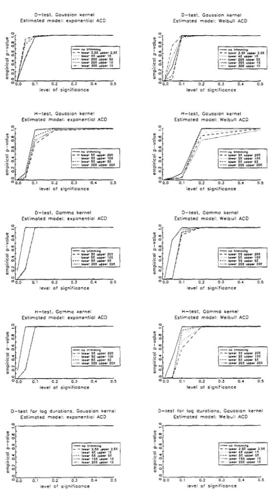
Figures 1 to 4 display the main results for n = 3000 using Davidson and

MacKinnon's (1998) graphical representation. Each figure consists of several

charts, which are set up in the same way. On the horiwntal axe is the

sig-nificance level and on the vertical axe is the probability of rejection at that

significance level. Ideally the size of a test, i.e. the probability of rejection

under the null, coincides with the significance leveI, whereas the power, i.e. the

probability of rejection under the alternative, is dose to one. To take size

distor-tions into consideration, we consider size-corrected power, i.e. the probability

of rejection given simulated rather than asymptotic criticaI values.

The performance of the D-test for log-standardised durations is a salient

feature in ali figures. The results are quite encouraging in that such testing

procedure is mildly conservative and have excellent power. Besides, the amount

of trimming does not seem to aifect these results. In fact, no trimming seems

other hand, the other four tests are to some extent disappointing. In

partic-ular, the inferior performance of tests based on gamma kernels are somewhat

surprising in view of the absence of bOtUldary bias. Such outcome may be due

to the inefficient criterion we have adopted to chose the bandwidth.

Figures 1 and 2 consider the case in which durations follow a Burr ACD

processo Figure 1 shows that both D- and H-tests using a Gaussian kernel fail

to entail good size performance. In particular, the H-test with Gaussian kernel

rejects in every instance the specification of the model, though it is correct.

Heavy trimming in the lower tail improves slightly the performance of the D-test,

but the distortions are still substantial. Using a gamma kernel, the probability

of rejection of the D-test is about 42% irrespective of the weighting scheme and

the leveI of significance at hand. A similar result is due to the H-test with

gamma kernel.

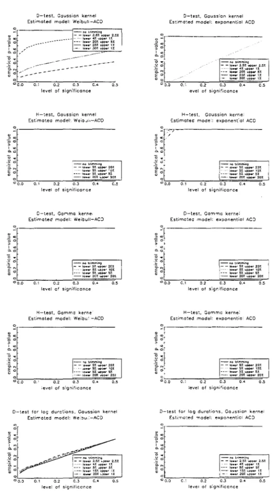
Figure 2 illustrates the fact that our tests have, in general, good power

against exponential (first column) and Weibull (second column) alternatives.

Using a Gaussian kernel, the D-test necessitates heavy trimming in the lower

tail, whereas the H-test requires trimming in the upper tail. The intuition is

simple. Density estimation with fixed kernels performs poorly dose to the origin

due to the boundary bias and thus deleting the observations in the lower tail

decreases distortions in the D-test. By the same token, pointwise estimates of

the hazard rate function are quite unstable in the upper tail because the survival

function approaches zero. Therefore, it is not surprising that a higher amount

of trimming is necessary in the upper tail for the H-test. Accordingly, the good

size-corrected power of both D- and H-tests with no trimming comes at the

expense of huge size distortions (see figure 1).

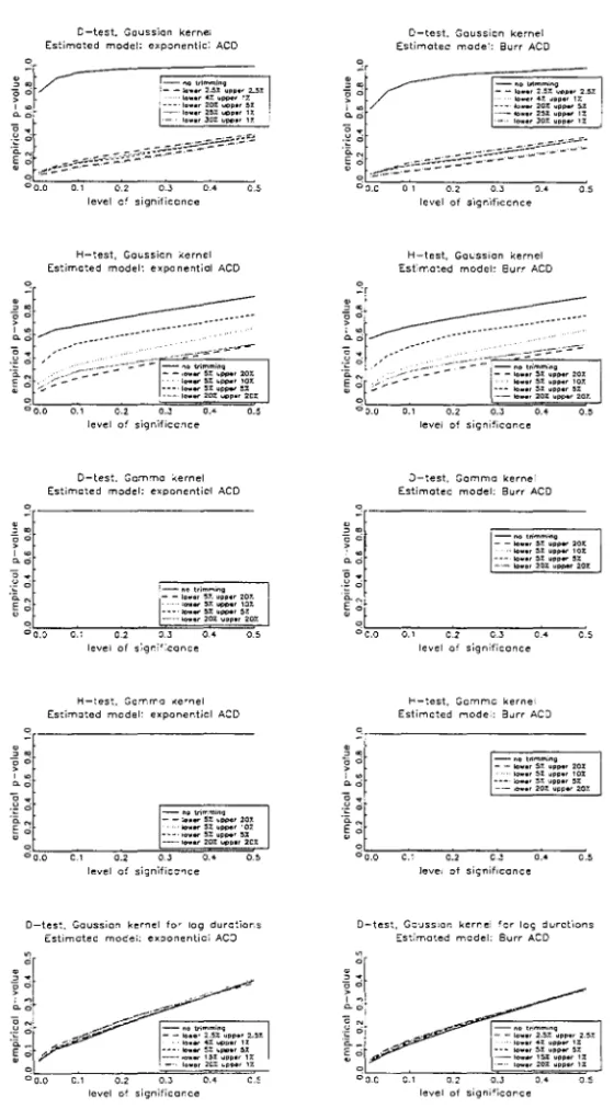
The first and second column of figure 3 document respectively the size and

power of our tests when standardised durations have a Weibull distribution.

The most striking feature in figure 3 is the complete failure of the D-test with

gamma kernel and both H-tests in terms of size performance. In turn, the

D-test using a Gaussian kernel performs reasonably well provided that severe

trimming is applied to the lower tail; power is trivial otherwise. The intuition

is two-fold. First, as aforementioned, this sort of trimming is necessary to

counteract the boundary bias of fixed kernel density estimation. Second, the

..

zero, the parametric estimates of the density approaches infinity as opposed to non-parametric estimates which are bounded. As such, squared differences can

get extremely large and the remedy is to introduce more trimming.

Figure 4 reveals that size distortions are less palpable when durations follow

an exponential ACD model. The D-test using a Gaussian kernel is slightly

more conservative than the D-test applied to log-standardised residuals. Severe

trimming in the upper tail is afresh essential to H-tests, though size distortions

remain material. Last but not least, our results accord with Grammig and

Maurer (1999) in that there is no increase in size distortions if the estimated

model considers a more general distribution than necessary. Differences are so

minor that we have opted to display only the case in which we estimate a Burr

ACD model, though the true distribution is exponential.

To conserve on space, we refrain from displaying similar graphs for the full

sample (n = 15000) in view that, on balance, the results bear great resemblance.

Nonetheless, we collect in table 1 the main statistics for the case in which the

data follow a Burr ACD modelo In particular, size distortions remain roughly

constant, whereas power improves mildly in general - major improvements take

place only for the H-tests. In alI, the D-test for log-standardised durations seem

to outperform the other variants we have proposed. Nonetheless, as the other

tests also entail reasonable size-corrected power, one may take advantage of

resampling techniques to mitigate size distortions.

6 Empirical application

In this section, we use real world data to test the performance ofthe linear ACD

model (32) with exponential, Weibull and Burr distributions. Data were kindly

provided by Luc Bauwens and Pierre Giot and refer to the NYSE's Trade and

Quote (TAQ) data set. Bauwens and Giot (1997 and 1998) and Giot (1999)

describe more thoroughly the data.

We focus on data ranging from September to November 1996. In

particu-lar, we look at price duration processes of five actively traded stocks from the

Dow Jones index: Boeing, Coca-Cola, Disney, Exxon, and IBM. Trading at the

NYSE is organised as a combined market maker/order book system. A

".

and quoting processes and providing liquidity. Apart from an opening auction,

trading is continuous from 9:30 to 16:00. Price durations are defined by

thin-ning the quote process with respect to a minimum change in the mid-price of

the quotes. We define price duration as the time interval needed to observe a

cumulative change in the mid-price of at least $0.125 as in Giot (1999).

For alI stocks, durations between events recorded outside the regular opening

hours of the NYSE as well as overnight spells are removed. As documented

by Giot (1999), price durations feature a strong time-of-day effect related to

predetermined market characteristics such as trade opening and closing times

and lunch time for traders. To account for this anomaly, we consider seasonally

adjusted price durations Xi = Xii e(ti), where Xi is the raw price duration in

seconds and e( .) denotes a daily seasonal factor which is determined by averaging

durations over thirty minutes intervals for each day of the week and fitting a

cubic spline with nodes at each half hour. The resulting (seasonallyadjusted)

price durations Xi serve then as input in the sequeI.

Table 2 reports some descriptive statistics for price durations. There are

two comIDon features across stocks: highly significant serial correlation and

some degree of overdispersion. That is not surprising: Indeed, ACD models are

precisely designed to deal with these stylised facts.

6.1 Estimation and test results

We invoke (quasi) maximum likelihood methods to estimate linear ACD models

with exponential, Weibull and Burr distributions. We address both in-sample

and out-of-sample performances by splitting the sample. More precisely, we

reserve the last third for out-of-sample evaluation. Table 3 SurnIDarises the

estimation results. For every stock, the Burr ACD model reveals a considerable

better fit as indicated by log-likelihoods. On the contrary, the gains in using

a Weibull rather than an exponential distribution are quite marginal in most

instances. To see why, it suflices to notice that the Weibull estimates of K, are

always close to one. In fact, it turns out that K,

<

1 for every Weibull ACD

model, implying that the hazard rate function decreases monotonically with the

standardised duration. Conversely, K, estimates are significantly greater than

one for alI Burr ACD models, what indicates non-monotonic baseline hazard

'.

distributions produce similar estimates for duration processes as opposed to _{Burr ACD models. For Boeing and IBM price durations, differences are indeed}

striking. All in alI, parameter estimates suggest substantial persistence in the

rate at which price changes.

Next, we evaluate the performance of the estimated ACD models

byexamin-ing both in- and out-of-sample standardised durations, which we hereafter refer

as residuals and forecast errors, respectively. Tables 4 to 6 portray the results of

the D- and H-tests, which are very much in line with Bauwens, Giot, Grammig

and Veredas's (2000) analysis rooted in density forecasting techniques. Table 4

reports the p-values of the D-test using a Gaussian kernel for log-standardised

durations. As fingered by the Monte Carlo investigation, there is no need for

trimming. Residual analysis favours clearly the Burr ACD model as it cannot

be rejected at conventionallevels of significance for Boeing, Coca-Cola, Disney

and Exxon price durations. Contrariwise, the exponential and Weibull

alterna-tives perform quite poorly for every stock, but the Coca-Cola. The linear ACD

model is rejected both in- and out-of-sample for IBM price durations

irrespec-tive of the distribution. Inspecting the other forecast errors, we find evidence

of misspecification only for Boeing and Disney price durations, what probably

refl.ects the presence of structural changes.1

Table 5 displays the outcomes of the D-test with Gaussian kernel for raw

standardised durations. We consider three weighting strategies. The first exerts

no trimming whatsoever, what should produce an extremely conservative test

given the results in section 5. Indeed, apart from a borderline result for the

Disney residuals of the Burr ACD model, such testing procedure always rejects

the null. The second scheme trims realisations out of the interval (x,l - x),

where x denote the empirical 0.025-quantile. As expected, besides some few

cases involving residuals of Burr ACD models, rejecting the null remains the

rule. Lastly, applying heavy trimming in the lower tail recovers by a long chalk

the figures in table 3. The only difference is that the Burr ACD model appear

now to produce Boeing forecast errors and IBM residuals that satisfy the null.

Of course, this is perchance an artifact due to the weighting procedure since

misspecification might occur precisely in the trimmed part of the distribution.

Table 6 documents once more how unreliable are H-tests using a Gaussian

kernel. Model specification is rejected in nearly alI cases even if we introduce

severe trimming in the upper tail as suggested in section 5. By the same token,

tests based on gamma kernels do not seem very informative. Indeed, alI

p-values are inferior to 0.0005, mirroring the flimsy finite sample properties of

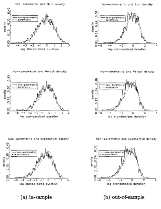
such tests. Figures 5 illustrates the results by plotting the non- and parametric

density estimates for Ex:x:on standardised durations. If, on the one hand,

non-parametric density estimates oscil1ate nicely around estimates from the Burr

ACD specification; on the other hand, parametric estimates implied by the

exponential and Weibul1 alternatives are consistently above or below their

non-parametric counterparts in some intervals.

For completeness, we check whether standardised residuals are serial

inde-pendent using the BDS test (Brock, Dechert, Scheinkman and LeBaron, 1996).

In contrast to the Ljung-Box statistic, the BDS test is sensitive not only to

serial correlation but also to other forms of serial dependence. Moreover, the

BDS test is nuisance parameter free for additive models (de Lima, 1996), what is

quite convenient given that we test estimated residuals rather than true errors.

A simple log-transformation renders the linear ACD model additive, hence it

suffices to work with log-standardised durations. Table 7 reports the results.

For the Boeing price durations, serial independence seems consistent only with

the residuals of the Burr ACD model. For Coca-Cola, ACD models seem to

produce serially independent residuals irrespective of the distribution, though

out-of-sample performances are poor. In turn, alI ACD models seem to capture

wel1 enough both in- and out-of-sample intertemporal dependence for Disney

price durations. Evidence is somewhat inconclusive for Ex:x:on price durations

by virtue of the multitude of borderline results. In contrast, the p-values for

the

ruM

log-standardised durations provide strong evidence against the serial

independence of both residuals and forecast errors.

Altogether, the figures in table 8 reinforce the evidence provided by the

D-test in tables 3 and 4. In particular, none of the linear ACD models seems to

fit properly

ruM

price durations. In turn, the Burr ACD model entails superior

performance relative to the exponential and Weibull ACD models for the other

--

1

Concluding remarks

This paper deals with specification tests for conditional duration models, though

there is no impediment in using such tests in other contexts. For instance, one

could test GARCH-type mo deIs by checking whether the distribution of the

standardised error is correctly specified. Similarly, Cox's (1955) proportional

hazard model implies testable restrictions in the hazard rate function. The main

reason to focus on conditional duration models stems from the poor performance

of quasi maximum likelihood methods in this context (Grammig and Maurer,

1999).

We propose two testing strategies, namely the D- and H-tests, which rely

on gauging the discrepancy between non- and parametric estimates of the

den-sity and baseline hazard rate functions of standardised durations, respectively.

Asymptotic theory is derived for non-parametric density estimation using both

fixed and gamma kernels. The motivation for the latter is to avoid the

bound-ary bias that plagues fixed kernel estimation. All in ali, our tests have some

attractive theoretical properties. First, they examine the whole distribution of

the standardised residuals instead of a limited number of moment restrictions.

Second, they are nuisance parameter free. Third, they are suitable to weak

dependent time series and, as such, there is no need to test previously for serial

independence of the standardised errors.

There are two main topics for future research. First, it is still unclear how

to select bandwidths for both fixed and gamma kernel estimations. A

possi-ble solution relies on cross-validation methods, which Chen (2000) shows to be

particularly valuable to gamma kernel estimation. More precisely, one builds

a grid of bandwidth values satisfying assumption A4 and then takes the

band-width that minimises the test statistic. Second, resampling techniques may

deliver more accurate critical values. Indeed, there is vast literature on

boot-strapping smoothing-based tests, e.g. Fan (1995) and Li and Wang (1998).

Under serial independence of the standardised residuals, the usual bootstrap

algorithm presumably works. Suitable bootstrap schemes are also available

un-der weak dependence, such as Poli tis and Romano's (1994) stationary bootstrap

and Bühlmann's (1996) sieve bootstrap, in case one prefers to relax the serial

"-Appendix: Proofs

Lemm.a 1. Consider the functional IG =

Io

oo CP.];

eix, where

Jx

=

j(x)

is a

pointwise gamma kernel estimate of

Ix

=

I(x).

Under assumptions AI, A2 and

A4,

b-1!4 ( )

nb1!41 - _n_ E [x- 1!2(fl ]

...!4

N O

~E

[X-

1!2(fl2 -r ]

n G

2ft

rX ,

ft

r x J X ,

provided that the above expectations existo

Proof. See Fernandes (1999).

Lemm.a 2. Suppose that a functional if!f is Fréchet-differentiable relative to

the Sobolev norro of order (2, m) at the true density function

I

with a regular

functional derivative cPf. Then, under assumptions AI to A4, n1!2 (if! /-if!f)

...!4

N

(O,

V~), where V", = 2:~-oo COV[cPf(Xi), cPf (Xi+k)] is the long run covariance

roatrix of cP f .

Proof. See Alt-Sahalia (1994).

Lemm.a 3. Consider a sequence {Xi : i

=

1, ... , n} that satisfies assumption

AI. Suppose that the U-statistic Un

==

2:1<i<j<n Hn(Xi, Xj) with symroetric

variable function Hn(·,·) is centred and degenerate. If

EX1,X2 {El1 [Hn(Xl,Xl)Hn(X1,X2)]}

+

~EX1,X2 [H~(Xl,X2)]

--~~~~~----~~~~~~~~--~~~~----~~O

Et,X2 [H;(X1,X2)]

as sample size grows, then

u

n

...!4

N

(o, n;

Ex1,X2

[H~(Xl,X2)])

.

Proof. See Hall (1984) and Khashiroov (1992).

Lemm.a 4. Consider the functional I =

Ix CPx!;

eix, where

Ix

denotes the

integral over the support of

x

and

!x

=

!(x)

is a pointwise fixed kernel estimate

of

Ix

=

I(x).

Under assumptions AI to A4,

provided that the above expectations are finite.

Proof. The derivation uses lemma 3, i.e. Khashimov's generalisation of Hall's

centrallimit theorero for degenerate U-statistics to weakly dependent

"-emergence of a degenerate U-statistic. Let rn(x, X) = cp~/2 Khn (x - X) and

Tn(X,X) = rn(x,X) - Ex [rn(x, X)] , where Khn (u) = h:;/ K(u/hn). Then,

I=

1

[trn(x,Xi)/T]

2

dx =

~2 ~

1

rn(x,Xi)rn(x,Xj)dx,

x ,=1 1.,3 x

or equivalently, I = II

+

12

+

13

+

14, where

h

=

:2

~

1

rn(x,Xi)rn(x,Xj)dx

'<J

12

~

L

r

r; (x, Xi)dx

n i

J",

We show in the sequeI that the first term is a degenerate U-statistic and will

contribute with the variance in the limiting distribution, whilst the second will

contribute with the asymptotic mean. In addition, the third and fourth terms

are negligible under assumption A4. The first moment of rn(x, X) reads

Ex [rn(x, X)] = cp;/2

Ix

Khn (x - X)f(X)dX = cp;/21 K(u)f(x

+

uhn)du

cp~/21

K(u) [f(X)

+

~f'(X)Uhn

+

!"(X*)U2h;] du

= cp~/2 f",

+

O (h;') ,

where fei) denotes the i-th derivative of f and x* E _{[x, x+uhn].} Applying similar

algebra to the second moment yields Ex [r~(x,X)] = h:;;1 eK cp",f", +0(1). This

means that

n-1h:;;,I eK

1

cp",f", dx

+

O (n- 1) ,

whereas Var(I2) = O (n-3_{h:;;2). It follows then from Chebyshev's inequality}

that nh?n/2 12 - 77;;1/2 eK E[cp",] = Op(I). In turn, we have that

14

=

n(n

~

1)

r

El

[rn(x, X)] dx

=

n(n

~

1) O

(h~)

=

O

(h~)

,

n

J",

n

which, under assumption A4, implies that nhlj2 14 = 0(1). Further,

E(I3 )

=

2(n -1)

1

Ex [rn(x, X)] Ex rn(x,X)] dx

=

O,

v [

--whilst E(I§) =

o

(n-

1

_h;).

_{It suffices then to impose assmnption A4 to}

en-sure, by Chebyshev's inequality, that nh;!2 l3

=

op(l). Finally, recall that

II = 2:i<j Hn(Xi,Xj ), where Hn(Xi,Xj) = 2n-2

I;,:

Tn(X,Xi)Tn(X,Xj)eIx. As

Hn(Xi,Xj) is symmetric, centred and such that E [Hn(Xi, X j ) IXj] = O almost

surely, II is a degenerate U-statistic. Thus, it follows immediately from lemma

3 that nh;!2

h

-'4

N(O, VH ), where

n4hn _[ 2 ]

VH

=

-2-Ex1,X2 Hn(XI,X2

=

2hn

r

[1

Tn(x,Xl)Tn(X,X2)eIx] 2 f(X1,X2)d(X1,X2)

JX1,X2 ;,:

=

2hn

l,y

[Ix

Tn(X,X)Tn(y,X)f(X)dXf d(x,y)

21,v

cp;

[lu

K(u)K(u

+

v)f(x - uhn) du

- hn

lu

K(u)f(x - uhn) du

lu

K(u)f(x

+

vhn - uhn) dU] 2 d(x,v)

21,v

cp;

[lu

K(U)K(U+V)f(X-Uhn)f d(x,v)

2VK

1

cp;

f;

eIx,

which completes the proof.

Proof of (10). Consider the following expansion

iJ! f,h(r) = iJ! f+,h =

fs

[f(x, O,) - f(x) - "(h(X)]2 [f(x)

+

"(h(x)] eIx,

where 0,

=

0f+,h. Differentiating with respect to "( yields

2

fs

af~O

O,)~;

[f(x, O,) - f(x) - "(h (x)] [f (x)

+

"(h (x)] eIx

- 2

fs

[f(x, O,) - f(x) - "(h(x)] [f(x)

+

"(h(x)]h(x) eIx

+

fs

[f(x, O,) - f(x) - "(h(x)]2 h(x) eIx.

Under the null, the parametric specification of the density function is correctly

specified, i.e. f(x,O)

=

f(x); hence the first functional derivative DiJ!f

=

"-2

r

8f(x,0-y) 8f(x, O-y) 80-y 80-y

[f

h ] dx

+

1

s 80 80'

a,

8,' '"

+, '"

- 4

r

8f(x,0-y) 80-y

[f

h ] h d

ls

80 8, '"

+, '" '"

x

r

8f(x,0-y) 80-y [ ]

+41s 80 8, f(x,O-y)-f",-,h", h",dx,

+

2 !s[f", +,h",] h; dx - 4 !s[J(x,o-y) - f", - ,h",] h; dx,

which reduces to (10) by evaluating at ,

=

o

and imposing the null.

Proof of Theorem 2. Under the null, the following functional Taylor

expan-sion is valid

\I!f+h =

1

lI.(x E S) [i7(x,y)

+

_{f",8C"') (y)] dH(x)H(y)}

+

O

(llh",11

3) ,

"',y

where i7 is a continuous functional which includes the first and second terms

of (10) as well as the regular part of its third term and 8C"') is a Dirac mass at

x. Replacing h", by

j", -

f", ensues that the first term

1

lI.(x E S)i7(x, y) dH(x)dH(y)

"',y

is negligible since it converges at a faster rate T to a sum of independent X2

distributions (Serfling, 1980; Ait-Sahalia, 1994). In turn, applying lemma 1 with

cp",

=

lI.(x E S)f", yields that

r

lI.(x E S)f",8C"')(y) dH(x)dH(y) =

1

f",h; dx

l""y

s

converges in distribution at rate nb;!4 to a Gaussian variate with mean b:;;1/4 8G

and variance O"~.

Proof of Theorem 3. The conditions imposed are such that the functional

Taylor expansion under consideration is valid even in case the Xin, i = 1, ... , n,

are a double array. Thus, for the D-test with fixed kernel, it ensues that, under

Hfn

and assumptions AI to A4,

nhl/2 1 n 2 dlnJ

f;; -

~-

E

lI.(Xin E S) [f(Xin,Of) - f(Xin)]

-+

N(O, 1),

O"D n i=l

where the superscript [n] denotes dependence on f[nl. The first result follows

plnJ

then by noting that Ô" D ~ O" D and

1 n 2

- E

lI.(Xin E S [f[nl (xin,OflnJ) - f[nl(Xin)]

". E { D.(Xln E S) [f[n1 (Xln' O/In)) - f[n1(xl n)

r}

+

Op

(n-1 /2)

c;'E

[D.(Xl n E S)lb(Xln)]

+

op

(n-

1h;1/2)

-lh-1/2nS

+

(-lh-

1/ 2 )

n n {.D op n n .

Applying a similar argument to the gamma kernel version of the D-test

com-pletes the proof (see the proof of theorem 7).

Proof of (18). Consider the following expansion

A/,h(J)

=

Af+-Yh

=

fs

[r9,

(x) -

r

f+-yh(X)]

2

[J(x)

+

'Yh(x)] dx,

where o-y = O f+-yh to simplify notation. Differentiating with respect to'Y entails

r

ar

9 (x) ao

=

2 ls a8 a;

[ro.,.

(x) -

r

f+-Yh(X)] [f(x)

+

'Yh(x)] dx

- 2

fs

ar

/~~h(X)

[ro.,.

(x) -

r

/+-yh (x)][f (x)

+

'Yh(x)] dx

+

fs

[ro.,.(x) -rf+,h(X)]2 h(x)dx,

which recovers (18) if evaluated at 'Y

=

o.

Proof of (20). Computing the second differential of the expression above with

respect to 'Y yields

r

a2ro.,. (x) ao, ao-y

= 2

18

aoao' a'Ya'Y' [r9.,.(X)-rf+-Yh(X)] [J(x)+'Yh(x)]dx

r

ar9.,.

(x) ~o-y [

+21s ao a'Ya'Y' ro.,.(X)-rf+,h(X)] [f(x)+'Yh(x)]dx

+

2

r

ar9.,.

(x)

ar9.,.

(x) ao-y ao-y [f( )

+

h( )] dx

ls ao ao' a'Y a'Y' x 'Y x

- 4

fs

ar~8(x)

a:;

ar

/~~h(X)

[f(x)

+

'Yh(x)] dx

r

ar9.,.

(x) ao-y [

+41s ao a'Y r9.,.(X)-rf+,h(X)]h(x)dx

- 2

r

a2r~+,~(x)

[ro.,.

(x) -

r

f+-Yh(X)] [J(x)

+

'Yh(x)] dx

ls 'Y'Y

+

2

r

ar

f+-yh

ar

f+-yh [f(x)

+

'Yh(x)] dx

ls a'Y a"('

- 4 lar

/~~h(X)

[r9.,.

(x) -

r

f+-yh(X)] h(x) dx,

Proof of Theorem 5. Under the null, the following functional Taylor

expan-sion is valid

A!+h =

1

n(x E S) [ef(x,y)

+

S;l Ó(X) (y)] dH(x)H(y)

+

O

(1IhW),

x,v

where

ef

is a continuous functional encompassing the second and third terms

of (20) as well as the regular part of its first term and Sx denotes the survival

function 1-F(x). Replacing hx by Jx - Ix ensues that the first term

l,y

n(x E S)ef (x,y) dH(x)dH(y)

converges at a rate T and therefore it is negligible. In turn, applying lemma 4

with r.px

=

n(x E S)S;l yields that

r

n(x E S)S;l Ó(x)(Y) dH(x)dH(y) =

r

S;lh; dx

Jx~

~

converges weakly at rate nhlj2 to a normal distribution with mean h;;1/2)\H

and variance

ç'h.

Proof of Theorem 6. Consider the above functional Taylor expansion with

hx

=

Jx - Ix' Once more, the first term converges at a rate T, whereas lemma

1 implies that

r

n(x E S)S;lÓ(x)(Y) dH(x)dH(y) =

r

n(x E S)lxh; dx

~~

~

converges in distribution at rate nblj4 to a normal variate with mean b;;1/4ÀG

and variance

çl;.

Proof of Theorem 7. Afresh, the corresponding functional Taylor expansion

is consistent with the double array sequence Xin, i

=

1, ... , n. Thus, for the

H-test with gamma kernel, we have that, under

Hfn

and assumptions AI to A4,

H nblj4 1 ~ 2 dlnl

Tn - - " - -~ n(Xin E S) [[(x, O,) -

r

,(x)] ~ N(O, 1).

çG n i=l

E { n(X1n E S)

[r[n

1 (X1n, O ,Inl) -

r~nl(x1n)

r}

+

Op

(n-

1/2)

ê;E [n(X1n E

S)e~(X1n)]

+

op

(n-

1b;;1/4)