A family of autoregressive conditional duration models

(1)

Nº 501

ISSN 0104-8910

A family of autoregressive conditional duration models

Marcelo Fernandes

Joachim Grammig

(2)

A Family of Autoregressive Conditional

Duration Models

Marcelo Fernandes

Graduate School of Economics, Getulio Vargas Foundation

Praia de Botafogo, 190, 22250-900 Rio de Janeiro, Brazil

E-mail: [email protected]

Joachim Grammig

Department of Economics, University of T¨ubingen

Mohlstr. 36, D-72074 T¨ubingen, Germany

E-mail: [email protected]

Abstract: This paper develops a family of autoregressive conditional

dura-tion (ACD) models that encompasses most speciﬁcadura-tions in the literature.

The nesting relies on a Box-Cox transformation with shape parameterλto the conditional duration process and a possibly asymmetric shocks impact

curve. We establish conditions for the existence of higher-order moments,

strict stationarity, geometric ergodicity and β-mixing property with

expo-nential decay. We next derive moment recursion relations and the

autoco-variance function of the powerλof the duration process. Finally, we assess the practical usefulness of our family of ACD models using NYSE

trans-actions data, with special attention to IBM price durations. The results

warrant the extra ﬂexibility provided either by the Box-Cox transformation

or by the asymmetric response to shocks.

JEL Classification: C22, C41.

Keywords: Asymmetry, Box-Cox transformation, mixing property, price

duration, shocks impact curve, stationarity.

Acknowledgements: We are grateful to the anonymous referee, Valentina

Corradi and David Veredas, as well as many seminar participants, for helpful

comments. The authors thank the ﬁnancial support from CNPq-Brazil and

(3)

1 Introduction

The seminal work of Engle and Russell (1998) hoisted a great interest in

the implications of price and trade durations in empirical ﬁnance. For

in-stance, the modeling of price duration processes hinges the approaches to

option pricing and intraday risk management recently proposed by Prigent,

Renault and Scaillet (2001) and Giot (2000), respectively. Although Engle

and Russell’s (1998) autoregressive conditional duration (ACD) model is the

starting point of such analyses, the literature carries several extensions.

Bauwens and Giot (2000) work with a logarithmic version of the ACD

model that avoids the nonnegativeness constraints implied by the original

speciﬁcation so as to facilitate the testing of market microstructure

hy-potheses. Bauwens and Veredas (1999) propose the stochastic conditional

duration process, leaning upon a latent stochastic factor to capture the

un-observed random ﬂow of information in the market. Ghysels, Gouri´eroux

and Jasiak (2003) introduce the stochastic volatility duration model to cope

with higher order dynamics in the duration process. Zhang, Russell and

Tsay (2001) argue for a nonlinear version based on self-exciting threshold

autoregressive processes.

This paper develops a family of ACD models encompassing most of the

existing models in the literature, such as the nonlinear ACD speciﬁcations

recently put forward by Dufour and Engle (2000). For that purpose, we

exploit the common features shared by the ACD and GARCH processes

and follow a similar approach taken by Hentschel (1995) to build a family of

asymmetric GARCH models. The nesting relies on a Box and Cox’s (1964)

transformation with shape parameter λ ≥ 0 to the conditional duration

(4)

latter stems from Engle and Russell (1998), who show that standard ACD

models applied to ﬁnancial data tend to overpredict after extreme (very long

or very short) durations.

We establish suﬃcient conditions for the existence of higher order

mo-ments, strict stationarity, geometric ergodicity andβ-mixing property with

exponential decay in this class of augmented ACD models. Although there

are no general analytical solutions for the autocorrelation function and

mo-ments of the duration process, we show that it is possible to derive the

autocovariance function and moment recursion relations for the powerλ of

the duration process. Alternatively, one must restrict attention to particular

subclasses, e.g. λ→ 0 and λ= 1, in order to work out expressions for any

arbitrary moment and the autocovariance function.

We then demonstrate the practical usefulness of our ACD family

model-ing IBM price durations and other ﬁnancial durations from stocks actively

trading on NYSE. Our ﬁndings clearly reject the restrictions imposed by the

existing models in the literature. Further, we show that allowing for a

con-cave shocks impact curve is paramount, because it mitigates the problem of

overpredicting short durations. It is thus no wonder that we ﬁnd some sort

of substitutability between the Box-Cox transformation and the asymmetric

eﬀects given that both may lead to concavity of the shocks impact curve.

The remainder of the paper is organized as follows. Section 2 outlines the

statistical properties of the family of augmented ACD processes. Section 3

collects the ﬁndings of the empirical application to NYSE transactions data,

focusing on IBM price durations. Section 4 summarizes the main results and

(5)

2 The augmented ACD model

Letxi =ti−ti−₁denote the time spell between two events occurring at times

ti and ti−1. For example, price durations correspond to the time interval

needed to observe a certain cumulative change in the stock price, whereas

trade durations stand for the time elapsed between two consecutive

trans-actions. To account for the serial dependence that is common to ﬁnancial

duration data, Engle and Russell (1998) formulate the accelerated time

pro-cess xi = ψiǫi, where the conditional duration process ψi =E(xi|Ωi−₁) is

stochastically independent of the iid sequence formed by ǫi and Ωi−₁ is the

set including all information available at timeti−₁. As in Hentschel (1995),

we generalize the ACD processes by applying a Box-Cox transformation with

parameterλ≥0 to the conditional duration process ψi, giving way to

ψ_iλ−1

λ =ω∗+α∗ψ

λ i−1

h

|ǫi−₁−b| −c(ǫ_i−₁−b) iυ

+βψ

λ i−₁−1

λ . (1)

The shape parameterλdetermines whether the Box-Cox transformation is

concave (λ≤1) or convex (λ≥1).

The augmented autoregressive conditional duration (AACD) model then

ensues by rewriting (1) as

ψ_iλ =ω+α ψλ_i−1 h

|ǫi−₁−b|+c(ǫ_i−₁−b) iυ

+β ψ_iλ−1, (2)

where ω = λω∗ −β+ 1 and α = λα∗. The AACD model provides a

ﬂex-ible functional form that permits the conditional duration process {ψi} to

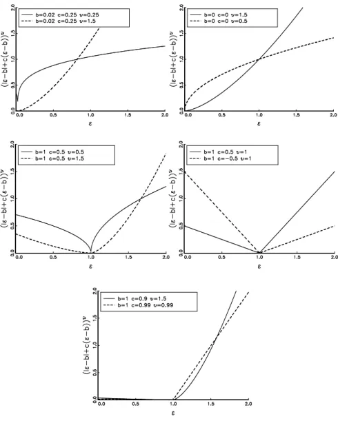
respond in distinct manners to small and large shocks. The shocks impact

curveg(ǫi) = [|ǫi−b|+c(ǫi−b)]υ incorporates such asymmetric responses

through the shift and rotation parametersband c, respectively.

Because durations are nonnegative, the shift parameter b is key to the

(6)

curve. In turn, the parameter c determines whether rotation is clockwise

(c < 0) or counterclockwise (c > 0). Interestingly, it is not necessarily the

case that shift and rotation reinforce each other. Indeed, the shift parameter

aﬀects mostly small shocks, whereas rotation is dominant for large shocks.

The shape parameter υ plays a similar role to λ, inducing either concavity

(υ≤1) or convexity (υ≥1) to the shocks impact curve. Figure 1 illustrates

the behavior of the shocks impact curveg(·) according to the values of the

shift, rotation and shape parameters.

Figure 1

The original ACD model of Engle and Russell (1998) is recovered by

imposing λ= υ = 1 and b =c = 0, whereas letting λ→ 0 and b= c = 0

renders the Box-Cox ACD speciﬁcation put forward by Dufour and Engle

(2000). Further, (1) reduces to Bauwens and Giot’s (2000) logarithmic ACD

models either if λ → 0, υ = 1 and b = c = 0 (Type I) or if λ, υ → 0 and

b = c = 0 (Type II). Following the GARCH literature, one may build

other conditional duration models by imposing restrictions on (1). The

examples we consider in the sequel include the asymmetric logarithmic ACD

(λ → 0 and υ = 1), asymmetric power ACD (λ = υ), asymmetric ACD

(λ = υ = 1), and power ACD (λ = υ and b = c = 0). Dufour and Engle

(2000) independently propose a version of the asymmetric logarithmic ACD

model with b = 1 under the name of exponential ACD model. We keep

our notation because the linear ACD model with exponential distribution is

sometimes referred to as the exponential ACD model. Table 1 summarizes

the typology of ACD models under consideration.

(7)

2.1 Properties

In this section, we build heavily on Carrasco and Chen’s (2002) general

re-sults to establish suﬃcient conditions that ensureβ-mixing and ﬁnite higher

order moments for (conditional) duration processes belonging to the

aug-mented ACD family. The ﬁrst step consists in casting (2) into a generalized

polynomial random coeﬃcient autoregressive model

Xi+1=A(ei)Xi+B(ei), i= 0,1,2, . . . (3)

where{ei}forms an iid sequence. Next, we apply Mokkadem’s (1990) result

for polynomial autoregressive models to derive the mixing properties of{ψi}.

For the duration process {xi}, we take advantage of Carrasco and Chen’s

result on the mixing properties of a processYi =Xi+εi, where Xi is a β

-mixing homogeneous Markov process andεiis an iid noise with a continuous

density. These two results are collected in Propositions 2 and 4 of Carrasco

and Chen (2002), respectively.

Proposition 1: Let xi =ψiǫi, where ψi satisfies (2) and ǫi is an iid

ran-dom variable that is stochastically independent of ψi. Assume further that

the probability distribution of ǫi is absolutely continuous with respect to the

Lebesgue measure on (0,∞) and such that the density is positive almost

everywhere. Suppose that |β|<1 and

E|β+α[|ǫi−b|+c(ǫi−b)]υ|m<1, (4)

for some integer m > 1. Then, {ψi} is a geometrically ergodic Markov

process and, if initialized from its ergodic distribution, is also strictly

sta-tionary and β-mixing with exponential decay. Further, E¡

ψ_iλm¢

< ∞ and

E¡

xλm i

¢

<∞. Condition (4) with m= 2 is also necessary to entail

geomet-ric ergodicity of{ψi}andE¡ψ2iλ ¢

(8)

distribution,{xi}is strictly stationary andβ-mixing with exponential decay.

Proof: The ﬁrst two results follow immediately from Carrasco and Chen’s

Proposition 2 with Xi = ψλi, A(ei) = β +α[|ǫi −b|+c(ǫi −b)]υ, and

B(ei) =ω, where ei= (|ǫi−b|, ǫi)

′

. The need for condition (4) withm= 2

stems from Lemma 2 of Pham (1986). The last result follows from Carrasco

and Chen’s Proposition 4 withYi= logxi,Xi = logψi, and εi = logǫi. ¥

If the interest were only in deriving suﬃcient conditions for the

dura-tion processes xi to be nondegenerate and covariance stationary, one could

alternatively use the tools provided by Nelson (1990, Theorems 1 to 3) as

in Hentschel (1995). Actually, for most of the models in the family spanned

by the augmented ACD process, the conditions in the proposition above

are both necessary and suﬃcient. The exceptions are formed by the models

that ascertain a positive conditional duration even when at least one of the

following restrictions are violated: ω > 0, α > 0, β > 0, and |c| ≤ 1 for

some odd integerυ. For instance, lettingλ→0 ensures nonnegativeness of

the duration process without imposing further restrictions.

For the sake of completeness, we establish similar properties for the ACD

models belonging to the family of augmented ACD processes. At ﬁrst glance,

it seems that it suﬃces to consider the parametric restrictions implied by

each model in condition (4) to extract the corresponding result. That is

not the case, though. To derive (4), one must impose restrictions on A(·)

and B(·), which vary according to the speciﬁcation of the model. More

speciﬁcally, Carrasco and Chen’s (2002) results require that|A(0)|<1 and

that, for some integerm≥1,E|A(ei)|m <1 andE|B(ei)|m <∞.

The generalized polynomial random coeﬃcient autoregressive

(9)

A(ei) = β, and B(ei) = ω +α[|ǫi −b|+c(ǫi −b)], implying that

con-dition (4) becomes E(ǫm

i ) < ∞. For the asymmetric power ACD model,

A(ei) =β+α[|ǫi−b|+c(ǫi−b)]λandB(ei) =ω, so that it suﬃces to impose

that E

¯ ¯

¯β+α[|ǫi−b|+c(ǫi−b)] λ¯¯

¯ m

<1. The latter condition also holds

for the asymmetric ACD model withλ= 1 and for the power ACD

speciﬁca-tion withb=c= 0. While the Box-Cox ACD process asks forE(ǫυm_i )<∞,

the logarithmic ACD models of Bauwens and Giot (2000) require either that

E(ǫm_i ) exists (Type I) or that |α+β|<1 and E|logǫi|m <∞ (Type II).

As advanced by Carrasco and Chen (2002), in the linear ACD model,

condi-tion (4) reduces toE|β+αǫi|m<1, which is equivalent to assuming that

α+β <[E(ǫm i )]

−₁_/m

is ﬁnite.

2.2 Higher-order moments and autocovariance function

In general, there is no analytical solution for the moments and

autocorrela-tion funcautocorrela-tion of duraautocorrela-tion processes belonging to the augmented ACD family.

Nonetheless, it is possible to derive moment recursion relations and the

au-tocovariance function of the power λ of the duration process by extension

of He and Ter¨asvirta’s (1999) results for the family of GARCH models.

To derive theλm-th momentµλmof the duration process, we write (2) in

its generalized polynomial random coeﬃcient autoregressive representation

ψ_iλ =Ai−₁ψ_iλ−1+B, (5)

whereB =ω and Ai =β+α g(ǫi). Raising both sides to the power m >0

and then applying recursions give

ψ_iλm=³Ai−1ψλ_i−₁+B ´m

=Am_i−₁ψ

λm i−₁+

m X j=1 µ m j ¶

BjAm−_j

i−₁ ψ

λ(m−_j₎

(10)

=ψ_imλ−n

n Y

k=1

Am_i−k+

m X j=1 µ m j ¶ n X k=1

BjAm−j

i−_k ψ

λ(m−_j₎

i−_k

k−₁ Y

ℓ=1

Am_i−ℓ. (6)

We are now ready to state the next proposition that documents moment

recursion relations for the augmented ACD class of processes.

Proposition 2: Let xi = ψiǫi, where ψi satisfies (5) with 0 < EAmi < 1

and{ǫi}is an iid process stochastically independent of{ψi}. Assume further

that the process started at some finite value infinitely many periods ago. It

then follows that

µλm=

Eǫλm i

1−EAm_i

m X j=1 µ m j ¶

Bj_EAm−j

i

Eǫλ_i(m−j) µλ(m−j) (7)

for some integer m≥1 and µ0= 1.

Proof: Because the process started at some ﬁnite value inﬁnitely many

periods ago, we can letn→ ∞in (6) and take expectations, resulting in

Eψ_iλm=Eψ_imλ(EAm_i )n+

m X j=1 µ m j ¶

BjEAm_i −jEψ_iλ(m−j)

n X

k=1

(EAm_i )k−₁

= 1

1−EAm i m X j=1 µ m j ¶

BjEAm_i −jEψ_iλ(m−j).

To complete the proof, it suﬃces to observe thatψi andǫi are stochastically

independent, and henceµλm=Eǫλmi Eψiλm. ¥

Before moving to the autocovariance function of the powerλof the

dura-tion process, two remarks are in order. First, assuming that 0< EAm i <1 is

analogous to imposing condition (4) in Proposition 1. Second, the moment

recursion relation in (7) involves moments that are possibly of fractional

order. Unfortunately, it is not possible to derive expressions for a moment

of an arbitrary order for such a general family of processes without

restrict-ing the shape parameterλof the Box-Cox transformation of the conditional

(11)

a recursion relation involving moments of any integer order. Alternatively,

one could also consider the subclass of conditional duration processes

deter-mined by the limiting caseλ→0. We follow the latter approach in the end

of this section in view that the log-transformation of the duration process is

quite convenient for avoiding nonnegativeness constraints.

Proposition 3: Letxi=ψiǫi, whereψi satisfies (5) with 0< EAmi <1for

some integer m≥2. Let ǫi form an iid sequence stochastically independent

of {ψi} such that EAiǫλi is finite. It then follows that the autocovariance

functionγλ,n=Exλixλi−_n−µ2_λ of order n≥1 reads

γλ,n=

B2_Eǫλ i

1−EAi 

 n−1 X

j=0

(EAi)j+

(EAi)n−1EAiǫλi(1 +EAi)

1−EA2

i

− Eǫ λ i

1−EAi 

. (8)

Proof: Multiplying both sides of (5) by ψ_iλ−_n yields

ψ_iλψλ_i−_n= ³

Ai−₁ψλ_i−₁+B ´

ψ_iλ−_n

=hAi−1 ³

Ai−2ψλ_i−₂+B ´

+Biψ_iλ−_n

=



B+B n X

j=2

j−₁ Y

k=1

Ai−_k+

n Y

k=1

Ai−_kψ_iλ−_n 

ψλ_i−_n.

Multiplying now both sides by ǫiǫi−_n and then taking expectations give

Exλ_ixλ_i−_n=Eǫ

λ iB



1 + n X

j=2

(EAi)j−1 

Eψ_iλ+Eǫλ_i(EAi)n −₁

EAiǫλiEψ2iλ

=Eǫλ_i



B Eψλ_i n−1 X

j=0

(EAi)j+ (EAi)n−1EAiǫλiEψi2λ 

.

The result then ensues from the fact that equation (6) implies that the

ﬁrst and second moments of ψλ

i are respectively Eψiλ =B/(1−EAi) and

Eψ_i2λ =B2(1 +EAi)/[(1−EAi)(1−EA2i)], whereas the moment recursion

(12)

As an example, consider the linear ACD process with an exponential

noise introduced by Engle and Russell (1998), which results from λ = 1,

Ai =β+αǫi andB =ω. Proposition 2 then implies that

µm=

Γ(m+ 1) 1−E(β+αǫi)m

m X j=1 µ m j ¶

E(β+αǫi)m−j

Γ(m−j) ω

j_µ m−_j

provided thatα+β <1. Solving for m= 1 and m= 2 yields the ﬁrst two

moments as derived in Engle and Russell (1998). In turn, it follows from

Proposition 3 that the autocovariance function of ordernreads

γn=ω2 ½

1−(α+β)n 1−(α+β) +

(α+β)n−₁

(1 +α+β)(2α+β) [1−(α+β)] [1−(α+β)2₋_α2_]

¾

.

This expression provides a sharper result than Bauwens and Giot’s (2000)

recursive formula for computing the autocovariance function of a linear ACD

process with exponential errors.

We now focus on a particular subclass of the augmented ACD family

that permits working out expressions for any arbitrary moment as well as

the autocorrelation function. This subclass is determined by shrinking the

Box-Cox shape parameter to zero (λ→0), yielding

logψi =ω+α g(ǫi−₁) +β logψ_i−₁. (9)

This subclass is particularly interesting for ensuring that the duration

pro-cess is always positive regardless of the sign and magnitude of the

pa-rameters. In particular, it nests the asymmetric logarithmic ACD model,

Bauwens and Giot’s (2000) logarithmic ACD speciﬁcations, and the Box-Cox

ACD process put forward by Dufour and Engle (2000). He, Ter¨asvirta and

Malmsten (2002) derive analogous results for a class of exponential GARCH

models.

To derive the m-th moment µm = Exmi of the duration process, it is

(13)

to the power m >0 and then applying recursions give

ψ_im= exp [m ω+m α g(ǫi−₁)]ψm β_i₋₁

= exp

Ã

m ω

n−₁ X k=0 βk ! _n Y k=1

exphm α βk−₁

g(ǫi−_k) i

ψ_im β−nn.

Assuming thatE{exp [κ g(ǫi)]}<∞forκ∈(0,∞) and that|β|<1, yields

Eψ_im = exp

µ

m ω 1 +β

n

1−β

¶ n Y

k=1

Enexphm αβk−₁

g(ǫi) io

Eψ_im βn. (10)

We are now ready to state the next result that reports them-th moment of

the duration process deﬁned in (9).

Corollary 1: Let xi =ψiǫi, where ψi satisfies (9) with |β|<1 and {ǫi} is

an iid process stochastically independent of {ψi}. Assume that the process

started at some finite value infinitely many periods ago. If both Eǫm_i and

E{exp [m α g(ǫi)]} are finite for some integer m≥1, it then follows that

µm=Eǫmi exp £

m ω(1−β)−₁¤ ∞ Y

k=1

Eexpnhm αβk−₁

g(ǫi) io

. (11)

Proof: Because the process started at some ﬁnite value inﬁnitely many

periods ago, we can letn→ ∞in (10), resulting in

Eψ_im= exp£

m ω(1−β)−₁¤ ∞ Y

k=1

Enexphm αβk−₁

g(ǫi) io

.

The result then follows from the fact that ψi and ǫi are stochastically

independent. ¥

Next we move to the autocovariance function of duration processes in

the (λ→0)-subclass of augmented ACD models. As before, the exponential

form of (9) facilitates the task.

Corollary 2: Let xi = ψiǫi, where ψi satisfies (9) with |β| < 1 and is

(14)

E{exp [α g(ǫi)]} and E{ǫiexp [α g(ǫi)]} are finite. It then follows that the

autocovariance function γn=Exixi−_n−µ2₁ of order n≥1 reads

γn=EǫiE©ǫiexp£αβn−1g(ǫi)¤ª n−1

Y

k=1

Enexphαβk−₁

g(ǫi) io

× ∞ Y

k=1

Enexphα(1 +βn)βk−₁

g(ǫi) io

exp

µ

2ω

1−β

¶

−µ2₁. (12)

Proof: Consider the exponential form of the conditional duration process

(9), then

ψiψi−_n= exp Ã

ω

n−₁ X k=0 βk ! _n Y k=1

exphαβk−₁

g(ǫi−k) i

ψβ_i−n_n+1,

which means that

xixi−_n=ǫ_iǫ_i−_nexp Ã

ω

n−₁ X k=0 βk ! _n Y k=1

exphαβk−₁

g(ǫi−_k) i

ψβ_i−n_n+1.

Taking expectations in both sides yields (12). ¥

3 Empirical application

In this section, we estimate diﬀerent ACD speciﬁcations using IBM price

durations at the New York Stock Exchange (NYSE) from September to

November 1996. Data were kindly provided by Luc Bauwens and Pierre

Giot, who have formed a broad data set using the NYSE’s Trade and Quote

database. We deﬁne price duration as the time interval needed to observe a

cumulative change in the mid-price of at least $0.125 as suggested by Giot

(2000). Price durations are closely tied to the instantaneous volatility of

the mid-quote price process (Engle and Russell, 1997 and 1998); hence it

is not surprising that they may have serious implications to option pricing

(Prigent et al., 2001) and intra-day risk management (Giot, 2000).

Apart from an opening auction, NYSE trading is continuous from 9:30 to

(15)

the regular opening hours of the NYSE, are removed. As documented by

Giot (2000), durations feature a strong time-of-day eﬀect. We therefore

consider diurnally adjusted durations xi =Di/̺(ti), where Di is the plain

duration in seconds and̺(·) denotes the diurnal factor determined by ﬁrst

averaging the durations over thirty minutes intervals for each day of the

week and then ﬁtting a cubic spline with nodes at each half hour. The

resulting (diurnally adjusted) durations serve as input for the remainder of

the analysis.

Table 2

Table 2 describes the main statistical properties of the IBM price

du-rations. We compute descriptive statistics for both plain and diurnally

ad-justed data. It takes on average 4.4 minutes for a cumulative price change of

$0.125 to take place, though the median waiting time is much lesser than 2

minutes. Overdispersion is robust to the time-of-day eﬀect, thus it is not an

artifact due to data seasonality. Sample autocorrelations reveal that

persis-tence is slightly changed if one accounts for the diurnal factor. Altogether,

the combination of overdispersion and autocorrelation in the price durations

warrants the estimation of autoregressive conditional duration models.

We then estimate by maximum likelihood the ACD models listed in

Table 1 assuming thatǫi is iid with Burr density

fB(ǫi; θB) =

κ µκ B,1ǫκ

−₁

i ³

1 +γ µκ B,1ǫκi

´1+1/γ, (13)

whereκ > γ >0 and

µB,m≡

Γ(1 +m/κ) Γ(1/γ−m/κ)

(16)

denotes the m-th moment, which exists for m < κ/γ. The Burr family

encompasses both the Weibull (γ →0), exponential (γ →0 andκ= 1), and

log-logistic (γ →1) distributions.

Table 3

Tables 3 and 4 report respectively the estimation results for the existing

models in the literature and the novel speciﬁcations. Asymptotic standard

errors are based on the outer-product-of-the-gradient (OPG) estimator of

the information matrix since the absolute value function in the shocks impact

curve makes Hessian-based estimates tricky to compute due to numerical

problems.

Table 4

It is interesting to observe that the estimates of the Burr parameters κ

andγ are quite robust regardless of the speciﬁcation of the duration process.

They imply that the baseline hazard rate function is nonmonotonic and that

there are at most three ﬁnite moments in view that ˆκ/γˆ ∈[2.7173,3.0438].

The parameter estimates of the linear and logarithmic ACD models are very

much in line with the previous results in the literature (see columns ACD,

LACD I and LACD II, respectively). Interestingly, the log-likelihood value

of the logarithmic ACD Type I model substantially diﬀers from the values

of the linear and logarithmic ACD Type II speciﬁcations. The

asymmet-ric logarithmic ACD model with b = 1 introduced by Dufour and Engle

(2000) palpably increases the log-likelihood value (-4,920.5 versus -4,950.5),

suggesting that asymmetry may play a role (see column EXACD). The last

column BCACD shows however that letting the powerυofǫi−₁ free to vary

(17)

value than introducing asymmetric eﬀects. Indeed, in the Box-Cox ACD

model, ˆυ is signiﬁcantly diﬀerent from both zero and one, lending some

support against the logarithmic ACD Type I and II models, respectively.

In the power ACD speciﬁcation, we notice that the shape parameterλof

the Box-Cox transformation is also signiﬁcantly diﬀerent from both zero and

one (see column PACD). This indicates that the restrictions imposed by the

linear and the logarithmic ACD Type I models seem inconsistent with the

data, even though the latter is only marginally inferior to the power ACD

model in terms of log-likelihood value. Introducing an asymmetric eﬀect to

the power ACD speciﬁcation ameliorates only marginally the ﬁt of the model

(see column A-PACD). Despite the fact thatbis signiﬁcantly diﬀerent from

zero, the standard error ofc is quite large, showing that the shocks impact

curve features no rotation. Although both shift and rotation parameters

are signiﬁcant in the asymmetric ACD speciﬁcation (see column A-ACD), it

violates the constraints usually imposed to ensure the nonnegativeness of the

duration process, namelyα > 0 and|c|<1. The A-LACD column shows

that all parameters are signiﬁcantly diﬀerent from zero in the asymmetric

logarithmic ACD model. In particular, given that ˆα is negative, the shift

and rotation eﬀects are such that the shocks impact curve is concave.

The ﬁgures displayed in the column AACD demonstrate that the

dou-ble Box-Cox transformation (λ6=υ) brings about further improvements as

indicated by the value of the log-likelihood of the augmented ACD model.

The diﬀerence between ˆυ and ˆλis striking. Indeed, there is strong evidence

supporting that λ converges to zero (i.e. the log transformation), whereas

0.1310<υ <ˆ 0.5178 with 99% of conﬁdence. The fact that ˆλis close to zero

(18)

From equations (1) and (2), it happens thatα=α∗λonly ifλ >0, whileα

and α∗ are equivalent in the limiting case λ→ 0. Table 4 reports ˆα = ˆα∗λˆ

and the corresponding standard error as computed by the delta method. It

is therefore straightforward to retrieve the estimate of α∗ from the ﬁgures

in Table 4: Indeed, ˆα∗ = 0.3898 with standard error equal to 0.1839.

To have a better idea about the ﬁt of the models, we undertake an

infor-mal log-likelihood comparison that accounts for overparameterization. We

do not pursuit a formal analysis based on log-likelihood ratio tests because,

due to the presence of inequality constraints in the parameter space, the

limiting distribution of the test statistic is a mixing of chi-square

distribu-tions with probability weights depending on the variance of the parameter

estimates (Wolak, 1991). Accordingly, it is extremely diﬃcult to obtain

empirically implementable asymptotically exact critical values. As an

alter-native, Wolak suggests applying asymptotic bounds tests. However, bounds

are in most instances quite slack, often yielding inconclusive results.

We compute the Akaike information criterion, AIC≡ −2(logL −k)/T,

where logLdenotes the value of the log-likelihood,kthe number of

param-eters andT the number of observations. In terms of AIC values, the horse

race winners are augmented ACD, the Box-Cox ACD, the asymmetric power

ACD, and the asymmetric logarithmic ACD models.1 _{The rewards of the}

extra ﬂexibility granted by these speciﬁcations are in contrast to the poor

performance of the linear and logarithmic ACD Type II models. Further,

letting λ free to vary and accounting for asymmetric eﬀects seem to

oper-ate as substitute sources of ﬂexibility. For instance, it is very rewarding to

1

(19)

introduce asymmetric responses to shocks in speciﬁcations with ﬁxedλ.

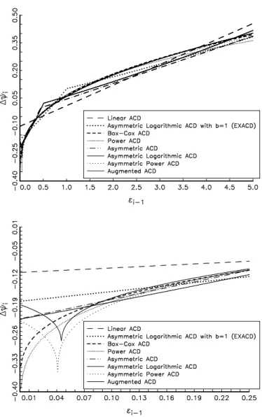
Figure 2

Figure 2 portrays the eﬀective shocks impact curves of each speciﬁcation

by depicting the variation of the conditional duration ∆ψi ≡ ψi−ψi−1 in

response to a shockǫi−₁at timet_i−₁. We ﬁx the conditional duration process

ψi−₁ at time t_i−₁ to one, while we vary the shock ǫ_i−₁ from zero to ﬁve.2

It is striking that, in all instances, ∆ψi reacts in a very similar fashion to

the shock. In particular, it seems that the concavity of the shocks impact

curve is the most important feature to account for when modeling IBM price

durations, alleviating the problem of overpredicting short durations. In the

sequel, we argue that the apparently substitutability between the Box-Cox

transformation and the asymmetric eﬀects is chieﬂy caused by the need to

achieve concavity of the shocks impact curve.

The asymmetric linear and logarithmic ACD’s shocks impact curves are

concave only for certain values of the shift and rotation parameters, namely

b >0 andc <−1. From this perspective, the parameter estimates reported

in the column EXACD in Table 3 and columns A-ACD and A-LACD in

Ta-ble 4 are not surprising. The estimates of the shift and rotation parameters

are signiﬁcantly diﬀerent from zero and inferior to minus one, respectively.

In contrast, if the shape parameter υ is inferior to one, both the Box-Cox

and augmented ACD models produce concave shocks impact curves. In the

case of the AACD, this holds regardless of the shift and rotation

parame-ters, hence it comes with no wonder that the corresponding estimates are

not jointly signiﬁcant in the AACD speciﬁcation. As the power ACD model

2

(20)

imposes λ = υ, the estimate of ˆλ sets in towards the estimates of υ in

the Box-Cox and augmented ACD models so as to entail a concave shocks

impact curve. The same happens with the asymmetric power ACD model,

despite the fact that, at ﬁrst glance, one could also induce concavity through

the shift and rotation parameters. It turns out, however, that to ensure a

concave shocks impact curve the absolute value of the rotation parameter

must exceed one, running counter to the nonnegativeness constraint.3

In-deed, the augmented ACD model avoids this problem by lettingλconverge

to zero, thereby mimicking the asymmetric logarithmic ACD speciﬁcation.

All in all, Figure 2 illustrates some of the pitfalls from the speciﬁc to

gen-eral modeling approach: There are various ways to achieve a concave shocks

impact curve that the data call for and failing to start from a suﬃciently

general speciﬁcation may point to quite misleading directions.

We now infer about the statistical properties of the duration processes by

checking whether they satisfy the suﬃcient conditions for strict stationarity

derived in Proposition 1. The aim is to illustrate how to use Proposition 1

for testing purposes. Maximum likelihood requires strict stationary of the

duration process to ensure consistency, hence estimates that violate either

|β| < 1 or (4) are not very reliable. In the linear ACD model, this is

equivalent to verifying whether|α+β|< µ−_B,m1/m<∞ for some integerm >

1. The second inequality poses no problem as µB,m exists form < κ/ˆ ˆγ =

3.0139. However, ˆα+ ˆβ = 0.9915, whereas m= 2 yields ˆµ−_B,1₂/2 = 0.4348. In

contrast, all other speciﬁcations seem to satisfy the suﬃcient conditions put

forth in Proposition 1. For both versions of the logarithmic ACD model,

3

(21)

condition (4) holds in view that |αˆ+ ˆβ| < 1 in Type I and |βˆ| < 1 in

Type II. Further, |βˆ| < 1 guarantees that both restricted (EXACD) and

unrestricted (A-LACD) versions of the asymmetric logarithmic ACD model

as well as the Box-Cox ACD process are strictly stationary. The power ACD

model requires thatE|β+α ǫλ_i|2 <1 for some integerm >1, which reduces

to|α+β|< µ_B,−1₂/_λ2 form= 2. The latter inequality is empirically satisﬁed

as the parameter estimates are such that 0.9738 = ˆα+ ˆβ <µˆ−1/2

B,2ˆλ = 1.0058.

Numerical results based on 10,000 Monte Carlo simulations also show that

(4) holds for the asymmetric ACD and asymmetric power ACD models. As

λ → 0 in the augmented ACD model, strict stationarity follows from the

fact that|βˆ|<1.

To check for misspeciﬁcation, we ﬁrst inspect whether the standardized

durations display any serial correlation by looking at the sample

autocorre-lation function of n-th order with n varying from 1 to 60. Tables 3 and 4

document that there is no sample autocorrelation greater than 0.05 (in

mag-nitude) irrespective of the speciﬁcation of the conditional duration process.

Moreover, the Ljung-Box statistics also show no evidence of serial

correla-tion in the residuals.4 We therefore conclude that the conditional duration

models are doing a great job of accounting for the serial dependence in the

IBM price durations.

Next, we apply Fernandes and Grammig’s (2003) D-test to gauge the

closeness between the parametric and nonparametric estimates of the

den-sity function of the residuals. Under the correct speciﬁcation of the

condi-tional duration process, both the parametric and kernel density estimates

4

(22)

of the residuals ˆǫi = ψ_ψˆiiǫi converge to the true Burr density. In contrast,

misspeciﬁcation gives rise to a mixture of Burr distributions since the

fac-tor ψi

ˆ

ψi

does not converge to one in probability. The kernel density estimate

will then converge to this mixture of Burr densities, whereas the parametric

estimate always belongs to the Burr family. The test statistic is thus

pre-sumably close to zero under the null, whereas it should be large under the

alternative. The motivation to apply the D-test is twofold. First, although

it is slightly conservative, the D-test entails excellent power against both

ﬁxed and local alternatives. Second, it is nuisance parameter free in that

there is no asymptotic cost in replacing errors with estimated residuals.

To avoid boundary eﬀects in the kernel density estimates due to the

non-negativeness of standardized durations, we work with log-residuals rather

than plain residuals. All nonparametric density estimates use a Gaussian

kernel, whereas the bandwidths are chosen according to an adjusted-version

of Silverman’s (1986) rule of thumb. The adjustment is necessary because

the asymptotic theory of the D-test requires a slight degree of

undersmooth-ing so as to avoid additional bias terms (see Fernandes and Grammig, 2003).

Despite the fact that the p-values of the D-test seem to decrease with the

degree of smoothing, the results are qualitatively robust to minor variations

in the bandwidth value.

The D-test results illustrate the rewards of the extra ﬂexibility provided

by the AACD family. There is no standard speciﬁcation that performs well

as seen in Table 3. At the 1% level of signiﬁcance, we soundly reject the

linear and logarithmic Type I ACD models, whereas we ﬁnd a borderline

result for the asymmetric logarithmic ACD model with b = 1 proposed by

(23)

ACD model, while rejecting the logarithmic ACD Type II speciﬁcation is

somewhat arguable given that the p-value is very close to 0.05. The ﬁgures

in Table 4 are much rosier: There is indeed no clear rejection, though we ﬁnd

a borderline result for the asymmetric ACD model at the 5% signiﬁcance

level. The D-test results also indicate that the asymmetric logarithmic ACD

speciﬁcation is the most successful model, achieving a quite large p-value.

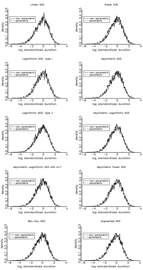
Figure 3 illustrates this pattern by plotting the kernel and parametric density

estimates of the log-residuals for the two groups of models in the ﬁrst and

second column, respectively. While there are striking discrepancies in the

ﬁrst column, the nonparametric density estimates nicely oscillate around the

parametric density estimates of the log-residuals in the second column.

Figure 3

To provide further empirical evidence, we consider price duration data,

from September to November 1996, relating to four actively traded stocks

on NYSE: Boeing, Coca-Cola, Disney, and Exxon. We also examine volume

and trade durations referring to the above stocks and IBM. Trade durations

measure the time between two successive transactions, whereas volume

du-rations denote the time interval needed to observe a cumulative trading

volume of 25,000 shares. We deal with intraday seasonality in the same

fashion as before. As expected, all durations keep featuring autocorrelation

and overdispersion even after adjusting for the time-of-day eﬀect.

Tables 5 to 7

Tables 5 to 7 respectively summarize the results for price, volume and

trade durations. We report the Akaike information criterion (AIC) and the

(24)

Restricting attention to the models that are not rejected by the speciﬁcation

tests, the horse race winners (according to the information criterion) belong

to the subclass of logarithmic ACD processes given by (9). In particular, we

select the LACD Type I model for the Boeing and Disney price durations as

well as for the Exxon volume duration data. Furthermore, the asymmetric

logarithmic ACD speciﬁcations (EXACD and A-LACD) perform well not

only for the Coke price and volume durations, but also for the Boeing

vol-ume duration. In contrast, we ﬁnd no suitable ACD speciﬁcation to model

either the IBM volume duration or any trade duration. The rejections are

mainly due to the residual serial dependence. We therefore deem that

fur-ther research must pay more attention to the logarithmic subclass of the

AACD family given that it is quite ﬂexible and easy to manipulate in the

context of higher order autoregressive structures.

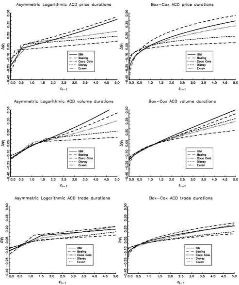
Figure 4

Lastly, the concavity of the shocks impact curve appears to be a quite

general feature of ﬁnancial duration data. Figure 4 displays the shocks

im-pact curves for the models with best overall performance. Although it seems

more pronounced for price durations, concavity shows up in all instances.

4 Conclusion

This paper introduces a family of augmented ACD models that

encom-passes most speciﬁcations in the literature. The nesting leans upon a

Box-Cox transformation to the conditional duration process and an

asymmet-ric shocks impact curve. The motivation for the latter stems from Engle

(25)

tends to overpredict after either very long or very short durations. We

de-rive suﬃcient conditions for the existence of higher-order moments, strict

stationarity, geometric ergodicity and β-mixing property with exponential

decay in this class of ACD models.

Our empirical results on IBM price durations show that the restrictions

imposed by the existing models in the literature are incompatible with the

data, warranting the extra ﬂexibility granted by the augmented ACD

mod-els. Actually, inspecting the parameter estimates of the diﬀerent

speciﬁca-tions reveals that imposing concavity in the shocks impact curve is pivot.

The Box-Cox transformation and the asymmetric response to shocks indeed

work, to some extent, as substitutes. In particular, the power ACD and

asymmetric logarithmic ACD models produce the best ﬁt.

Further empirical investigation reveals that the concavity of the shocks

impact curve is not a speciﬁc feature of the IBM price durations. Our

ﬁndings evince the same concave pattern using other ﬁnancial duration data,

(26)

References

Bauwens, L., Giot, P., 2000, The logarithmic ACD model: An application to

the bid-ask quote process of three NYSE stocks, Annales d’Economie

et de Statistique 60, 117–150.

Bauwens, L., Veredas, D., 1999, The stochastic conditional duration model:

A latent factor model for the analysis of ﬁnancial durations,

forthcom-ing in Journal of Econometrics.

Box, G. E. P., Cox, D. R., 1964, An analysis of transformations, Journal of

the Royal Statistical Society B 26, 211–243.

Carrasco, M., Chen, X., 2002, Mixing and moment properties of various

GARCH and stochastic volatility models, Econometric Theory 18, 17–

39.

Dufour, A., Engle, R. F., 2000, The ACD model: Predictibility of the time

between consecutive trades, University of Reading and University of

California at San Diego.

Engle, R. F., Russell, J. R., 1997, Forecasting the frequency of changes

in quoted foreign exchange prices with the autoregressive conditional

duration model, Journal of Empirical Finance 4, 187–212.

Engle, R. F., Russell, J. R., 1998, Autoregressive conditional duration:

A new model for irregularly-spaced transaction data, Econometrica

66, 1127–1162.

Fernandes, M., Grammig, J., 2003, Nonparametric speciﬁcation tests for

conditional duration models, Graduate School of Economics, Getulio

Vargas Foundation.

Ghysels, E., Gouri´eroux, C., Jasiak, J., 2003, Stochastic volatility duration

models, forthcoming in Journal of Econometrics.

Giot, P., 2000, Time transformations, intraday data and volatility models,

(27)

He, C., Ter¨asvirta, T., 1999, Properties of moments of a family of GARCH

processes, Journal of Econometrics 92, 173–192.

He, C., Ter¨asvirta, T., Malmsten, H., 2002, Moment structure of a family of

ﬁrst-order exponential GARCH models, Econometric Theory 18, 868–

885.

Hentschel, L., 1995, All in the family: Nesting symmetric and asymmetric

GARCH models, Journal of Financial Economics 39, 71–104.

Mokkadem, A., 1990, Propriétés de mélange des modèles autoregressifs

poly-nomiaux, Annales de l’Institut Henri Poincar´e 26, 219–260.

Nelson, D. B., 1990, Stationary and persistence in the GARCH(1,1) model,

Econometric Theory 6, 318–334.

Pham, D. T., 1986, The mixing property of bilinear and generalised

ran-dom coeﬃcient autoregressive models, Stochastic Processes and Their

Applications 23, 291–300.

Prigent, J.-L., Renault, O., Scaillet, O., 2001, An autoregressive

condi-tional binomial option pricing model, in: H. Geman D. Madan S. Pliska

T. Vorst (eds), Selected Papers from the First World Congress of the

Bachelier Finance Society, Springer Verlag, Heidelberg.

Silverman, B. W., 1986, Density Estimation for Statistics and Data Analysis,

Chapman and Hall, London.

Wolak, F. A., 1991, The local nature of hypothesis tests involving inquality

constraints in nonlinear models, Econometrica 59, 981–995.

Zhang, M. Y., Russell, J. R., Tsay, R. S., 2001, A nonlinear autoregressive

conditional duration model with applications to ﬁnancial transaction

(28)

(29)

(30)

(31)

(32)

Table 1

Typology of ACD models

Augmented ACD

ψ_iλ=ω+α ψ_iλ−₁ h

|ǫi−₁−b|+c(ǫ_i−₁−b) iυ

+β ψλ_i−₁

Asymmetric Power ACD (λ=υ)

ψλ

i =ω+α ψiλ−1 h

|ǫi−1−b|+c(ǫi−1−b) iλ

+β ψλ i−1

Asymmetric Logarithmic ACD (λ→0 andυ= 1)

logψi =ω+α h

|ǫi−₁−b|+c(ǫ_i−₁−b) i

+β logψi−₁

Asymmetric ACD (λ=υ= 1)

ψi =ω+α ψi−₁ h

|ǫi−₁−b|+c(ǫ_i−₁−b) i

+β ψi−₁

Power ACD (λ=υ and b=c= 0)

ψ_iλ=ω+α xλ_i−₁+β ψ

λ i−₁

Box-Cox ACD (λ→0 andb=c= 0)

logψi =ω+α ǫυi−₁+β logψi−₁

Logarithmic ACD Type I (λ, υ→0 and b=c= 0)

logψi =ω+α logxi−₁+β logψ_i−₁

Logarithmic ACD Type II (λ→0,υ= 1 and b=c= 0)

logψi =ω+α ǫi−₁+β logψ_i−₁

Linear ACD (λ=υ= 1 and b=c= 0)

(33)

Table 2

Descriptive statistics

IBM price durations plain adjusted

sample size 4,484 4,484

mean 262.55 1.239

median 128 0.714

maximum 7170 29.121

minimum 1 0.004

overdispersion 1.610 1.330

n-th order sample autocorrelation

n= 1 0.256 0.179

n= 2 0.231 0.184

n= 3 0.240 0.166

n= 4 0.168 0.121

n= 8 0.127 0.106

n= 12 0.095 0.099

n= 16 0.061 0.072

n= 20 0.018 0.062

n= 24 0.021 0.073

n= 28 0.000 0.050

n= 32 -0.008 0.047

(34)

Table 3

Estimation results for the AACD family of models IBM price durations ($0.125 mid-price change)

parameter ACD LACD I LACD II EXACD BCACD

ω 0.0171 0.0774 -0.0865 -0.0964 -0.5230

(0.0038) (0.0069) (0.0063) (0.0131) (0.1708)

α 0.1116 0.1250 0.0912 -0.1157 0.5843

(0.0088) (0.0083) (0.0067) (0.0152) (0.1768)

β 0.8799 0.8327 0.9759 0.9614 0.9616

(0.0089) (0.0127) (0.0042) (0.0064) (0.0067)

υ 0.2371

(0.0772)

c -1.4927

(0.1288)

κ 1.2616 1.3036 1.2592 1.2892 1.2954

(0.0318) (0.0331) (0.0318) (0.0327) (0.0330)

γ 0.4186 0.4808 0.4137 0.4519 0.4635

(0.0471) (0.0487) (0.0469) (0.0478) (0.0486)

logL -4,952.4 -4,924.8 -4,950.5 -4,924.5 -4,920.5

AIC 1.6836 1.6742 1.6830 1.6741 1.6728

D-test 0.0029 0.0025 0.0488 0.0140 0.0266

Q(4) 0.1965 0.0845 0.1152 0.5821 0.4990

Q(8) 0.0898 0.1433 0.1136 0.2410 0.2327

Q(16) 0.0836 0.0534 0.1569 0.1956 0.1891

Q(24) 0.0496 0.0897 0.1084 0.2853 0.2698

max ACF 0.0326 0.0403 0.0344 0.0370 0.0378

min ACF -0.0282 -0.0264 -0.0259 -0.0310 -0.0320

(35)

Table 4

Estimation results for the AACD family of models IBM price durations ($0.125 mid-price change)

parameter PACD A-ACD A-LACD A-PACD AACD

ω 0.0378 0.0208 0.0217 0.0378 0.0361

(0.0067) (0.0049) (0.0147) (0.0061) (0.0064)

α 0.1352 -0.1990 -0.2294 0.1270 0.00001

(0.0110) (0.0452) (0.0448) (0.0268) (0.1022)

β 0.8386 0.9760 0.9639 0.8468 0.9639

(0.0123) (0.0168) (0.0062) (0.0116) (0.0891)

λ 0.1751 0.2573 0.00003

(0.0848) (0.0681) (0.2621)

υ 0.3244

(0.0747)

b 0.4456 0.5066 0.0411 0.0451

(0.0741) (0.0680) (0.0019) (0.0015)

c -1.4294 -1.3172 0.2326 0.1117

(0.1099) (0.0724) (0.9446) (1.1718)

κ 1.2976 1.2882 1.2926 1.2979 1.2935

(0.0331) (0.0328) (0.0329) (0.0330) (0.0329)

γ 0.4688 0.4556 0.4589 0.4685 0.4588

(0.0487) (0.0484) (0.0485) (0.0482) (0.0483)

logL -4,922.7 -4,930.1 -4,921.1 -4,921.0 -4,918.4

AIC 1.6735 1.6760 1.6730 1.6729 1.6721

D-test 0.0955 0.0494 0.4039 0.1353 0.1370

Q(4) 0.3011 0.1794 0.4259 0.3866 0.5031

Q(8) 0.2085 0.0600 0.1182 0.2100 0.1840

Q(16) 0.1447 0.0719 0.1124 0.1447 0.1726

Q(24) 0.2224 0.1085 0.1536 0.2262 0.2594

max ACF 0.0378 0.0351 0.0352 0.0386 0.0381

min ACF -0.0301 -0.0341 -0.0370 -0.0316 -0.0331

(36)

Table 5

Estimation results for price durations ($0.125 mid-price change)

ACD LACD I LACD II EXACD BCACD PACD A-ACD A-LACD A-PACD AACD

Boeing sample size: 1,746 observations

AIC 1.9989 1.9759 2.0030 1.9890 1.9770 1.9771 1.9945 1.9815 1.9789 1.9800

Q(1) 0.551 0.734 0.210 0.539 0.732 0.708 0.754 0.585 0.736 0.679

Q(12) 0.320 0.219 0.460 0.353 0.220 0.221 0.484 0.417 0.214 0.225

D-test 0.103 0.173 0.006 0.283 0.157 0.160 0.113 0.140 0.121 0.097

Coke sample size: 1,072 observations

AIC 1.8885 1.8823 1.8909 1.8811 1.8833 1.8833 1.8923 1.8827 1.8863 1.8882

Q(1) 0.138 0.233 0.224 0.232 0.132 0.137 0.139 0.206 0.131 0.135

Q(12) 0.502 0.482 0.608 0.501 0.436 0.435 0.506 0.494 0.430 0.434

D-test 0.615 0.059 0.733 0.270 0.250 0.250 0.624 0.184 0.360 0.369

Disney sample size: 1,439 observations

AIC 2.2148 2.2104 2.2146 2.2127 2.2118 2.2118 2.2176 2.2130 2.2145 2.2159

Q(1) 0.926 0.869 0.874 0.877 0.866 0.856 0.889 0.836 0.833 0.848

Q(12) 0.685 0.500 0.673 0.543 0.524 0.512 0.670 0.430 0.514 0.519

D-test 0.133 0.271 0.213 0.371 0.295 0.281 0.188 0.087 0.295 0.303

Exxon sample size: 1,810 observations

AIC 1.9556 1.9521 1.9554 1.9549 1.9532 1.9533 1.9536 1.9529 1.9535 1.9545

Q(1) 0.219 0.241 0.267 0.232 0.234 0.267 0.149 0.231 0.304 0.304

Q(12) 0.228 0.265 0.251 0.224 0.250 0.258 0.208 0.308 0.272 0.272

D-test 0.099 0.006 0.136 0.043 0.029 0.033 0.091 0.017 0.012 0.012

(37)

Table 6

Estimation results for volume durations (cumulative trading volume: 25,000 shares)

AIC 1.8016 1.8054 1.7990 1.7983 1.8000 1.8021 1.8046 1.7999 1.8044 1.8063

Q(1) 0.964 0.762 0.831 0.772 0.802 0.935 0.898 0.724 0.850 0.849

Q(12) 0.537 0.367 0.586 0.516 0.542 0.510 0.551 0.503 0.515 0.516

D-test 0.573 0.478 0.767 0.781 0.703 0.567 0.507 0.790 0.610 0.607

AIC 1.8031 1.8060 1.8022 1.7993 1.8009 1.8018 1.8014 1.7994 1.8023 1.8033

Q(1) 0.033 0.029 0.031 0.064 0.057 0.053 0.072 0.091 0.062 0.060

Q(12) 0.096 0.006 0.096 0.059 0.066 0.065 0.054 0.052 0.052 0.053

D-test 0.390 0.834 0.137 0.499 0.634 0.658 0.696 0.691 0.636 0.631

AIC 1.8913 1.8967 1.8924 1.8915 1.8918 1.8918 1.8941 1.8907 1.8943 1.8960

Q(1) 0.364 0.130 0.284 0.329 0.358 0.364 0.352 0.330 0.368 0.367

Q(12) 0.524 0.297 0.524 0.463 0.493 0.494 0.526 0.517 0.483 0.493

D-test 0.000 0.010 0.000 0.002 0.000 0.000 0.000 0.000 0.000 0.000

AIC 1.6471 1.6400 1.6486 1.6404 1.6413 1.6413 1.6435 1.6416 1.6438 1.6453

Q(1) 0.732 0.456 0.947 0.486 0.446 0.446 0.526 0.535 0.417 0.435

Q(12) 0.575 0.572 0.587 0.593 0.573 0.572 0.598 0.598 0.563 0.593

D-test 0.886 0.989 0.818 0.961 0.964 0.964 0.909 0.987 0.962 0.962

IBM sample size: 2,869 observations

AIC 1.8300 1.8393 1.8282 1.8264 1.8259 1.8286 1.8311 1.8271 1.8274 1.8280

Q(1) 0.000 0.000 0.001 0.001 0.001 0.000 0.000 0.001 0.000 0.000

Q(12) 0.000 0.000 0.000 0.000 0.000 0.000 0.000 0.000 0.000 0.000

D-test 0.811 0.894 0.941 0.856 0.580 0.866 0.812 0.860 0.664 0.649

(38)

Table 7

Estimation results for trade durations

AIC 2.0765 2.0754 2.0762 2.0730 2.0733 2.0736 2.0738 2.0730 2.0733 2.0735

Q(1) 0.000 0.000 0.000 0.000 0.000 0.000 0.000 0.000 0.000 0.000

Q(12) 0.001 0.000 0.001 0.000 0.000 0.000 0.000 0.000 0.000 0.000