Alexander Dauwe,mst16000136
Faculdade de Economia: Finance Universidade Nova de Lisboa
Mentor: Prof. Paulo Leiria Mentor: Prof. Marcelo Moura
12 June, 2009
Abstract
1
Introduction
The main objective of this report is to evaluate the performance of a Principal Component forecast model when forecasting the Euro Interest Rate Swap curve for different time horizons. Specifically, its Root Mean Squared forecast Error (RMSE) will be compared with the results of though competitor models such as the Random Walk and the Nelson Siegel forecast model. Furthermore, the basic Principal Component forecast model will be extended with macro factors, in order to study the effect of Macroeconomic information on the forecastablility of the Euro Swap curve. Finally, first difference and Dickey Fuller adaptations of the original models will be postulated and evaluated.
Understanding the movements and being able to make accurate forecasts of the interest rates is crucial amongst bond portfolio management, monetary policy, debt policy,. . . The importance of yield curve forecasting, together with the fact that the Euro Swap market has become one of the largest and most liquid markets in the world, makes forecasting the Euro Swap curve very exciting.
This report contributes to the current term structure forecasting literature by evaluating a macro factor augmented Principal Component forecast model for the Euro Swap curve. In addition, new adaptations of the Nelson Siegel forecast model and the Principal Component forecast model have been developed, tested and evaluated. While testing the new models, the Nelson Siegel forecast model has been evaluated in a newer U.S. Treasury data set. Finally, an easy to use Matlab GUI program has been developed for forecast testing of various methods in flexible conditions.
This report consists of six sections. The first section will give a summary of all the yield forecasting literature that has contributed to this work. The next section will present the methodology that has been used to develop the Matlab GUI yield forecasting program. Section three will present and discuss the data. In the fourth section, I will present and discuss the results of the forecasting exercise. I conclude this work in section five. Finally, the sixth section is an appendix that contains all of the forecast tables that have been referred to in this work.
2
Literature Review
In this section I will present a specific selection of the most important term structure forecast research papers. However, before I do this, I will present the main target and motivation of many researchers to aboard this subject.
Due to the very high persistence of the yields, the naive ’no change’ model, also known as the random walk, is very successful at forecasting the term structure. However, evidence exists that the current term structure contains information about future term structures. As an example, Duffee (2002) states that long-maturity bond yields tend to fall over time when the slope of the yield curve is steeper than usual. Next to this internal evidence, the success of, for example, Taylor rules, has demonstrated a strong connection between the yield curve and the observable macro variables. Although the evidence is there, and many improvements have been made during the past decade, none of the researchers have succeeded yet in finding a single model that consistently outperforms the random walk for all forecast horizons and for all maturities.
that are important references for this work. I have structured them according to their core discussion points, in chronological order. Please note that some of the release dates are not consistent with the time the content of the paper became public knowledge.
2.1 Fundamental Research
In 2002 Duffee (Duffee, 2002) reports that the popular ”completely” affine/linear term struc-ture models do not perform well at forecasting. He discovers that this poor result is caused by the models fundamental assumption that the market price of the risk is a fixed multiple of the variance of the risk. By relaxing this assumption, Duffee creates a new model that seems to outperform the random walk. In this new ’essentially’ affine model, the market price of risk is no longer a fixed multiple of the variance of risk, but a linear combination of the state vector. Duffee names this model ”essentially” affine, because only the variance of the market price of risk loses its linearity in relation with the state vector.
In 2003 Ang and Piazzesi (2003) derive a no-arbitrage affine/linear term structure model, in which the state vector contains both observable macro factors and unobservable latent factors. Ang and Piazzesi are able to forecast the term structure by assuming that the dynamics of the state space vector are driven by a Gaussian VAR process. This paper is very original because it demonstrates a way to include macro variables directly into the term structure model. Important results of the paper are that the no-arbitrage restriction improves the forecast results and that macro factors explain up to 85% of the movements in the short and middle parts of the yield curve. In a one month ahead forecast exercise, their Macro model seems to beat the Random Walk.
In 2005 M¨onch (2005) follows a similar procedure to Ang and Piazzesi. He also uses the combination of no-arbitrate affine/linear model and a VAR of the state vector to forecast the interest rate term structure. Differences lie within the state vector. M¨onch uses the short term interest rate and the first four principal components of a large panel of macroeconomic time series. He justifies the use of factors by proving that the Fed’s monetary policy is better simulated with a Taylor rule based on macro factors, instead of macro variables. In relation to forecasting the term structure, M¨onch reports that relative to the random walk, his model reduces RMSE up to 50% at the short end of the term structure and still up to 20% at the long end.
2.2 Refinement research
Although many researchers report outperforming the random walk, none of them prove the consistency of their model. In 2007 de Pooter et al. (2007) set up a showdown between the Random walk, the original Nelson Siegel model (with and without macro factors) and the no-arbitrage models (with and without macro factors). Interestingly, the authors are not able to select the best model. Mainly because the forecast accuracy of each model is inconsistent over time. Their answer to making a better model, lies in determining logical combinations of all of the models. More specifically, they combine forecast models with a weighting scheme that is based on relative historical performance. Results are now consistent and highly accurate, especially for longer maturities. In relation with the macro factors, the authors notice a positive effect on out-of-sample forecasting.
Another attempt to use model selection is made by Blaskowitz and Herwatz (2008). The importance of this paper to this current work lies in that fact that the authors also implement the combination of a principal component yield curve model and an autoregressive model (AR). In addition, they too study the Euribor Swap Term Sturcture (Daily rates). Their adaptive technique consists of first creating a pool of models, by changing the time window, the number of principal components and the lags in the AR, next evaluating past performance of all of the models in the pool and finally selecting the best model to make the future forecast. They conclude that the adaptive approach offers additional forecast accuracy in terms of directional accuracy and big hit ability over the random walk and the Diebold and Li approach. However, the mean squared error results are not compared.
Next to disagreement in model selection, authors also do not yet agree on how to extract the macro factors. In 2008 Exterkate (2008) addresses this area. He evaluates the effect of different macro extraction techniques on the forecast performance of a Nelson Siegel model combined with a factor augmented VAR. Exterkate studies the effect of grouping macro variables before factor extraction and the effect of a technique called thresholding. The latter selects the macro variables with the highest forecasting potential. Exterkate reports a positive effect from both techniques. Next to this small victory, Exterkate has to report that including macro factors did not improve his forecast results compared to the original Diebold and Li setup. Additionally, he is not able to reproduce results that were previously achieved.
2.3 The role of No-Arbitrage restrictions
2.4 This report
Important lessons to be learned from the literature review: First, Duffee (2008) proves that, for a three factor discrete-time Gaussian model, the imposition of no-arbitrage onto the factors does not improve the forecasts. Second, de Pooter et al. (2007) shows that including the factors of macro variables into the factor transition equation has a positive result on the forecasts for all of his models.
This work exploits these results. I will use an unrestricted three-factor model, based on the principal components of the interest rate data, together with an autoregressive transition equation. In addition, I will include macro factors into the transition equation.
In the next section of this report, I will specify the autoregressive principal component model of the term structure in detail.
3
Methodology
Tests have shown that naive (vector) autoregressive models of the yields do not make use of the internal structure of the data when forecasting and that they produce bad forecast accuracy compared to the Random Walk (de Pooter et al., 2007). On the other hand, some models impose restrictions that do give better forecast results. Most of these successful models, impose restrictions on the parameters of a general linear yield curve model:
Yt = A+BXt+ǫt (1)
Xt = Γ1Xt−1+. . .+ ΓlXt−l+ηt (2)
The first equation models the yield curve, the second its dynamics. In this equation, Yt = [y1t, . . . , ynt]′ is the yield vector at time t, m denotes the number of maturities, Xt = [x1t, . . . , xnF t]′ is the state vector and l denotes the number of lags that are included in the transition equation. This general model assumes that each yield is a linear combination of nF factors from the state vector Xt. All yield curve models that I will discuss in this section are created by imposing a different constraint on A,B, Γ and the number of factors
nF inXt.
The main focus of this section is to explain how to specify equations (1) and (2) in case of the principal component model. I will do this in what follows, then I will generalize the model for macro factors, next I will discuss the implementation of the model and finally, I will present a summary of all the models that are used in this report.
3.1 Principal Component Model of the Term Structure
Principal component analysis (PCA) is defined as a linear transformation of a number of correlated variables into a smaller number of uncorrelated variables called principal com-ponents. Basically, making a principal component analysis comes down to computing the eigenvalues/eigenvectors of the covariance/correlation matrix of the variables. The main goal of this subsection is to apply this fundamental analysis onto the yield data and create the low dimensional factor format of the yield curve, similar to equation (1).
3.1.1 The algorithm
The idea behind principal component analysis is to determine the linear combination of vari-ables that has the highest variance. This linear combination of varivari-ables forms a new variable that is called ”component” or ”factor” (xit =α′iYt) and the coefficients of the linear combi-nation are called loadings (αi). In order to get a unique solution, the euclidian norm of the loadings must be fixed. In literature, the norm is arbitrarily fixed at one. The principal factor is discovered by maximizing the following problem:
var(X1) = var(α′
1Y) =α′1Y Y′α1 =α′1Σα1
||α1|| = α′1α1 = 1
With Σ being the covariance matrix of the dataY = [Y(τ1), Y(τ2), ..., Y(τm)]′ and α1 being
the loading of the first factor. Maximizing the variance of the linear combination of the variables comes down to solving the following Lagrange equation.
L = α′
1Σα1−λ1(α′1α1−1) (3)
Its solution is found by differentiating (3) in relation toα1 and λ1:
α′
1α1−1 = 0
(Σ−λ1Im)α1 = 0
These equations demonstrate that the factor with the highest variance, has the coefficients of the eigenvector that corresponds to the highest eigenvalue (α1 =B1P C) of the data variance matrix (λ1). The next step is to look for a second factor, which has unit length and which is orthogonal to the first factor (cov(α′
2Yt, α′1Yt) = 0). This leads to the following Lagrange system:
L = α′
2Σα2−λ2(α′2α2−1)−φλ1α′2α1 (4)
0 = Σα2−λ2α2−φλ1α1 (5)
Note that multiplying (5) withα′
2 reduces it to:
α′
2Σα2−λ2α′2α2−φλ1α′2α1 = 0
(Σ−λ2Im)α2 = 0
Again, the characteristic eigenvalue equation appears. This time the loadings of the second factor are determined by the eigenvector (α2 = B2P C) that corresponds with the second highest eigenvalue (λ2). This process can be continued until the rank of the data variance
matrix is reached. Beyond the rank, eigenvalues are zero and we can assign orthogonal eigenvectors arbitrarily. With real data, the eigenvalues are rarely zero due to noise.
The whole principal component algorithm can be summarized by making an eigenvector analysis on the data covariance matrix:
Σ = Y Y′=B′
P CΛBP C
Xt = α1 α2 ... αm
′Y
t=BP C′ Yt (6)
Remember that the principal component factors are independent and are extracted from the data in a natural way. If the no-arbitrage condition lies within the data, it does not need to be imposed when forecasting (Duffee, 2008).
Also note thatXtstill has the same dimension as the yields Yt. In the next section I will discuss why and how it is possible to reduce the dimension ofXt.
3.1.2 Reducing the dimension of the state vector
Inverting equation (6) 1 and then splitting up Xt is particularly helpful to understand how and why principal components can be used to reduce the dimensionality of the data. Let’s also look at a regression equation of the factors onto the yields:
Yt = B1P Cx1t+B2P Cx2t+. . .+BmP Cxmt (7)
Yt = Γ0+ Γ1x1t+ Γ2x2t+...+ Γmtxmt+ǫt (8)
Due to equation (7), regression(8) will explain all of the variance in Yt. In addition all coefficients will be estimated as Γ0 = 0 and Γi = BiP C, for all i different than 0. The potential to reduce the number of variables in this equation lies in the fact that the principal components are independent (orthogonal). This means that omitting a variable does not cause bias on the other coefficients and that each factor contributes a specific independent part toR2:
var(bijP CXj) = bijP CXjXj′bijP C =λjb2ijP C
var(Yi) =
X
var(bijP CXj) =
X
j=1:m
λjb2ijP C
X
i=1:m
var(Yi) =
X
j=1:m
λj
With Yi = [yi1, . . . , yit] and Xi = [xi1, . . . , xit]. It is now straightforward to identify and eliminate the factors that have a low contribution to the model. Moreover, without running the regression, each relatively low λi identifies a factor that can be eliminated from the equation (7), with minimum loss of accuracy. As discussed before, eigenvalues close to zero, are due to noise, so eliminating their corresponding factor in equation (7) is beneficial, as it reduces the noise in the yield data.
If a factor is truly important depends on the required model accuracy. In what follows next, I will discuss three automatic factor selection methods that I have implemented in my Matlab GUI program. First I will discuss the Kaiser criterium, next the Scree plot and finally the mean square error.
Kaiser-Guttman criterium The Kaiser-Guttman criterium was first proposed by Kaiser in 1960 (Field, 2009) and suggests only to keep factors with eigenvalues that are greater than one. The idea behind this criterium is that we only use a factor if it has more variance than an original variable. This method requires standardized variables with unit variance. Without standardized variables, this criterium can be applied when using an eigenvalue decomposition of the correlation matrix instead of the covariance matrix. In the context of interest rates, I use the correlation matrix to evaluate the Kaiser-Guttman criterium.
1Eigenvectors are orthogonal soB′
Scree plot The Scree plot (Field, 2009) plots the ordered eigenvalues in a Y/X plot, with X representing the number of the eigenvalue and Y representing its value. The name ”scree” comes from that fact that the plot looks like the side of a mountain, and ”scree” refers to the debris fallen from a mountain and lying at its base. The test is visual and proposes to stop including components at the point where the mountain ends and the debris begins.
Mean Square Error The error between the data (Yt) and the approximation ( ˜Yt) is given by:
Yt−Y˜t =
X
i=t:m
BiP Cxit
ΣErr
m−t =
X
i=t:m
λiBiP CBiP C′
m−t (9)
Withi being the number of all components that were not used in the approximation. Note that in equation (9),BiP CBiP C′ is a matrix and that the diagonal elements of Σ
Err
m−t+1 represents
the Mean Square Approximation Error. Another interesting fact is that the tray ofBiP CBiP C′ is one. This means that the mean of the Mean Square Approximation Error over all data is only determined by the eigenvalues that are not incorporated in the model:
mean(M SQE(Err)) = P
i=t:mλi
m−t
The idea of automatically determining the number of factors with the mean square error, can be achieved by setting a threshold mean square error.
When implementing these methods, I get values ranging from 2 to 3. Although the number of factors is just a variable which I can change in my program, most of the calculations have been made withnF = 3. Three factors is also common in literature.
3.1.3 Modifying the principal components
Next to the original setup, factor analysis suggests three modifications.
1. Subtracting the mean from the data does not change the covariance of the data and thus not the principal component analysis. It does change the factors and gives them a zero mean.
Yt−Yt = BP CX0t+ǫt
Yt−Yt
= BP CX0t=X0t= 0 (10)
Note thatX0trepresents the equivalent factors with zero mean. Because the eigenvectors are all independent, equation (10) only has a solution if all factors have a zero mean.
2. A second trick gives the factors unit variance. Due to the fact that the unit length of the eigenvectors is somewhat arbitrarily chosen, it is possible to scale the eigenvectors in such a way that the variance of the factors is one. This is done by multiplying the eigenvectors by the square root of their eigenvalue.
Yt−Yt =
X
i=1:nF
BiP C
p
λi
xi
0t √
λi
=B0P CX00t+ǫt
var(X00) = X00X00′ =
X0X0′
√
With X00t an equivalent factor with zero mean and unit variance. Note that the √
Λ and dividing by Λ is a short notation for implying that the operation is performed on each element of the matrix. Im represents a unit matrix with a size equal to the number of data series. Leaving out factors is easy and it just reduces the size of Im.
3. It is possible to apply linear transformations onto the loadings to improve their econom-ical interpretation. Imagine that the loadings span a subspace in the data space, then any set of vectors that can also span that subspace are equivalent to the loadings, with-out loss of accuracy. In general the idea is to look for vectors that have more economical meaning than the current loadings. In this master thesis I have tested the varimax ro-tation on the three principal factors of the term structure. The results are not shown because the rotation of the loadings did not enhance their economical interpretability.
3.2 Transition equation
Many authors use a vector auto regression models to forecast the factors. This, in order to catch the cross information between the factors. When using principal components however, the factors are not correlated. To be sure that also the lagged values of different factors are also not correlated, I have made the following regression:
xit = β1+β2xjt−1+ǫt for i6=j
None of the coefficients were significantly different from zero at a 5% level. Even with more than one lag, coefficients were never significantly different from zero. I therefore opt for an simpler auto regressive transition model:
Yt+h = BP CXt+h+ǫt
xit+h = β1+β2xit+...+βl+2xit−l+ηt for i = 1 :nF
With l the number of lags and nF the number of factors that are included in the model. Due to the fact that some of the factors are not stationary and have a unit root, I propose two alternative transition equations. The first alternative is to use an AR model on the 1st difference of the factors:
Yt+h = BP CXt+h+ǫt
Xt+h = Xt+ (Xt+h−Xt) =Xt+ ∆Xt+h
∆xit+h = β1+β2∆xit+...+βl+2∆xit−l+ηt for i = 1 :nF
The second alternative is to difference the data and use an AR on the principal components of the differences.
Yt+h = Yt+ (Yt+h−Yt) =Yt+ ∆Yt+h ∆Yt+h = BP CXt+h+ǫt
xit+h = β1+β2xit+...+βl+2xit−l+ηt for i = 1 :nF
3.3 Generalized Macro Forecast model
One of the important conclusions of de Pooter et al. (2007) concerning the forecast accuracy, is that including Macroeconomic information is beneficiary. In order to include macroeconomic variables into the principal component set up, I adapt two technique from the literature:
1. Diebold et al. (2004) suggest to incorporate the macroeconomic variables only in the transition equation of the state. In their set up, they augment the latent variables ’Level’, ’Slope’ and ’Curvature’ with manufacturing capacity utilization, the federal funds rate and annual price inflation. M¨onch (2005) discusses the advantage of working with the first few principal components of all macro data instead of working with actual macroeconomic variables.
2. Both M¨onch (2005) and Ang and Piazzesi (2003) include macro factors directly into their yield model.
Due to the flexibility of the principal component forecast model, adaptations of both versions can be tested. Version 1:
Yt+h = BP CXt+h+ǫt
xit+h = β1+β2xit+. . .+βl+2xit−l+
X
j=1:nM
(αj1mjt+. . .+αjkmjt−k) +ηt for i = 1 :nF (11)
with αi being a vector of parameters and Mt = [m1t, . . . , mnM t]′ being a array of macro factors. k denotes the lags for the macro factors. Note that equation (11) is an AR on the levels. In my matlab program I have also included the two alternative versions of the transition equations. In the second macro model, I combine yield and macro variables before applying principal components2. Version 2:
Y Mt+h = BP CXt+h
xit+h = β1+β2xit+. . .+βl+2xit−l+ηt for i = 1 :nF
With Y Mt+h being a vector that contains first the yields and then the macro factors. An advantage of this model is that due to the independence of the principal components, I can use a classical autoregressive model for the transition of state. Again, the Matlab GUI program also tests the alternative transition equations.
3.4 Out-of-sample forecasting
In this subsection I will describe how I have implemented the out of sample forecast scheme and how I have evaluated the performance of the forecast models.
3.4.1 Forecast Scheme
Imagine having a time seriesX = (x1, . . . , xn) on which you want to apply an autoregressive model and make out-of-sample forecasting. The first step to achieve ’testable’ out-of-sample
forecasting is to divide X into an in-sample part Xin = (x1, . . . , xm) and an out of sample part Xout= (xm+1, . . . , xn).
The autoregressive model is fully specified when the forecast step h and the number of lags l are known. In-sample we get the following regression:
xt+h = β1+β2xt+...+βl+2xt−l+ǫt for t =l+ 1 :m−h
For this regression to be in-sample, both the left hand side and the right hand side of this equation need to be in-sample, hence the domain oft. The next step is to use the coefficients of this equation to make an out-of-sample forecast. There are many ways to do this, but for this report, I only use in-sample observations of Xin to make the out-of-sample forecast with the following equation:
˜
xt+h = β1+β2xt+...+βl+2xt−l for t =m−h+ 1 :m
Note that the number of out-of-sample forecasts (domain of t) depends on the considered time step. In the Matlab program, I only retain the first out-of-sample forecastxm+1.
Other out-of-sample forecast are made by moving the history. In this report, I estimate the model with a ”rolling” history and with an ”increasing” history. A ”rolling” history has a fixed length and moves through time e.g. history1 = (x1, . . . , xm), history2 = (x2, . . . , xm+1),. . .
An ”increasing” history has an increasing length in time e.g. history1 = (x1, . . . , xm),
history2 = (1, . . . , xm+1),. . .
For each history, the principal components are calculated, regressed and used for one out-of-sample forecast as described. Note that this process is quite time consuming.
3.4.2 Evaluation
It is now time to quantify the error we make. I will first discuss the performance of a specific model and then the relative performance between nested models.
Performance All methods are both evaluated in-sample and out-of-sample. I use the mean square forecast error to determine the accuracy of the forecast model.
M SQEini −sample = X t=l+1:m−h
Yt+h−Y˜t+h
lhistory i=m, . . . , n−h
M SQEin−sample = mean(M SQEini sample)
M SQEout−of−sample =
X
t=m−h+1:n−h
Yt+h−Y˜t+h
lhistory
Note that in-sample, there areimean square errors due to the fact that the history is moving.
Relative Performance When more then one model is used, it is quite natural to want to rank them. For nested models, in which one model is a specific case of a more general model, West and Clark (2006) have developed a specific statistic based on the squared errors:
ft+h = (Yt+h−Y˜1t+h)2−
(Yt+h−Y˜2t+h)2−( ˜Y1t+h−Y˜2t+h)2
with ˜Y1t+h being the estimation of the nested model and ˜Y2t+h being the estimation of the more general model. In order to know if the general model is significantly better than the nested model, just regress ft+h on a constant for the out-of-sample domain and check if a is significantly larger than zero. In this work, I have used Matlabs 95% confidence intervals. If the lower bound is still larger than zero, the general model is better than the nested model. Specifically, in our case, the nested model is the Random Walk.
3.5 Summary of the models
This report compares the Principal Component Forecast Model with the Random Walk and the Diebold and Li Model. Next follows a brief description these three methods.
3.5.1 Principal Component Forecast Model
In this work I use four adaptations of the principal component forecast model called: PC AR, PC DAR, DPC AR and PC REG.
PC AR
Yt+h = BP CXt+h+Mt+ǫt
xit+h = β1+β2xit+...+βl+2xit−l+
X
j=1:nM
(αj1mjt+. . .+αjkmjt−k) +ηt for i = 1 :nF
WithBP C being a specific set of eigenvectors of the covariance matrix of the data,Mtbeing the mean of the in sample time series of Yinsamp ,h being the forecast step and l being the number of lags. It is important to realize that the principal component model only imposes restrictions onA = 0 andB =BP C in equation (1). These restrictions come naturally from the eigenvalue/eigenvector decomposition of the covariance in the data. Note that I have also implemented a Dickey Fuller version of this model. This model assumes the Random Walk in stead of the AR process if the seriesXi has a unit root.
PC DAR Regression of the differences of the principal components.
Yt+h = BP CXt+h+ǫt
Xt+h = Xt+ (Xt+h−Xt) =Xt+ ∆Xt+h ∆xit+h = β1+β2∆xit+...+βl+2∆xit−l+
X
j=1:nM
(αj1mjt+. . .+αjkmjt−k) +ηt for i = 1 :nF
DPC AR Regression of the principal components of the differenced matrix.
Yt+h = Yt+ (Yt+h−Yt) =Yt+ ∆Yt+h
∆Yt+h = BP CXt+h+ǫt
xit+h = β1+β2xit+...+βl+2xit−l+
X
j=1:nM
PC REG Direct regression of the parameters onto the yields.
yjt+h = β1+
X
i=1:nF
(βi2xit+...+βil+2xit−l) +
X
j=1:nM
(αj1mjt+. . .+αjkmjt−k) +ηt
3.5.2 The Random Walk
This model assumes that the best way to forecast future yields is to look at their current value:
Yt+h = Yt+ηt
With h being the forecast step. Due to the fact that interest rates have very high autocor-relations, the Random Walk model is very accurate. Remember that de Pooter et al. (2007) report that separately none of the models they tested consistently outperforms the Random Walk.
3.5.3 Diebold and Li Model
The 2002 Diebold and Li (2006) forecast model is a three factor dynamic Nelson Siegel model that imposes exponential restrictions on parameterB of equation (2). Diebold and Li specified the model as follows:
yt(τ1)
yt(τ2)
.. .
yt(τN)
= 1 1 .. . 1
C1t+
1−e−τ1λt
τ1λt
1−e−τ2λt
τ2λt
.. .
1−e−τN λt
τNλt
C2t+
1−e−τ1λt
τ1λt −e
−τ1λt
1−e−τ2λt
τ2λt −e
−τ2λt
.. .
1−e−τN λt
τNλt −e
−τNλt
C3t+
ǫt(τ1)
ǫt(τ2)
.. .
ǫt(τN)
Yt = BN SXt+ǫt
xit+h = β1+β2xit+. . .+βl+2xit−l+ηt for i = 1 : 3
Some important facts about the Diebold an Li model:
1. λt is a fourth parameter that determines the speed of decay of the elements in the coefficient B. Although this parameter may vary with time, Diebold and Li give it a fixed value based on the data.
2. All loadings are time independent. This enhances the speeds of out-of-sample forecasting dramatically.
3. The original transition equation is auto-regressive even though the Nelson Siegel factors are not independent and even though some have a unit root.
NS AR Diebold et al. (2004) propose the following scheme to include the macro variables:
Yt+h = BN SXt+h+ǫt
xit+h = β1+β2xit+...+βl+2xit−l+
X
j=1:nM
With Mt being the macro factor matrix and nM being the number of macro factors. Note that the transition equation has changed into a VAR. Due to the fact that the purpose of this paper is not to test transition equations, I will continue to use an autoregressive transition equation augmented with macro factors. Another difference from the original implementation, lies in the use of macro factors instead of macro variables. The implementation of the macro factors will be discussed later in this section.
NS DAR I also implement a Nelson Siegel model based on the differences:
Yt+h = BN SXt+h+ǫt
Xt+h = Xt+ (Xt+h−Xt) =Xt+ ∆Xt+h
∆xit+h = β1+β2∆xit+...+βl+2∆xit−l+
X
j=1:nM
(αj1mjt+. . .+αjkmjt−k) +ηt for i = 1 : 3
PC REG Direct regression of the parameters onto the yields:
yjt+h = β1+
X
i=1:nF
(βi2xit+...+βil+2xit−l) +
X
j=1:nM
(αj1mjt+. . .+αjkmjt−k) +ηt
Next up, a detailed discussion of the principal component method and its application to forecast the yield curve.
4
Data
Forecast literature has mainly dealt with the US treasury market because of the U.S. market dominance and because of its relatively large historical database. Nevertheless, in 2003 Re-molona and Wooldridge (2003) point out that the euro interest rate swap market has become one of the largest and most liquid financial markets in the world. As a consequence the swap yield curve is becoming a benchmark yield curve in euro financial markets, against which even government bonds are now often referenced. In this work, I put the main focus on forecasting the euro swap yield curve, but I also forecast the US treasury curve in order to compare my results with literature results and to justify that all of the forecast models are implemented correctly.
In what follows next I will first describe the US Treasury data, then the Euro Interest Rate Swap data and finally the European macroeconomic data.
to use the database of Gurkaynak et al. (2007). According to Bauer, this is nowadays the most commonly used database for U.S treasury yield curve research.
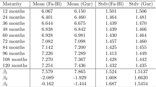
Although this database is not the identical to the database used by Diebold and Li, it does contain very similar data. Specifically, Diebold an Li used the unsmoothed Fama-Bliss continuously compounded zero yields from January 1985 up to December 2000 for the maturities of 3, 6, 9, 12, 15, 18, 21, 24, 30, 36, 48, 60, 72, 84, 96, 108 and 120 months. The Gurkaynak et al. (2007) database consists of continuously compounded zero-coupon yields which have been interpolated with a four factor Svenson model. Maturities range from 1 up to 30 years and the database contains daily data form 1961 to present. For this work, I have extracted monthly zero-coupon U.S. Treasury yields with maturities 12, 24, 36, 48, 60, 72, 84, 96, 108 and 120 months, over the period of January 1985 until February 2009. In the results section of this work, I will show that for similar conditions I get results similar to the results of Diebold and Li (2006). Table 1 reports the mean and standard deviation for all maturities. This, in order to demonstrate the slight difference between the Fama-Bliss yields and the Gurkaynak et al. (2007) yields. Note that the difference in values for β1, β2 and
Maturity Mean (Fa-Bl) Mean (Gur) Stdv(Fa-Bl) Stdv (Gur)
12 months 6.067 6.150 1.501 1.506
24 months 6.401 6.460 1.464 1.481
36 months 6.644 6.675 1.439 1.470
48 months 6.838 6.842 1.439 1.466
60 months 6.928 6.981 1.430 1.464
72 months 7.082 7.098 1.457 1.460
84 months 7.142 7.200 1.425 1.455
96 months 7.226 7.289 1.413 1.449
108 months 7.270 7.367 1.428 1.442
120 months 7.254 7.436 1.432 1.435
β1 7.579 7.865 1.524 1.5137
β2 -2.089 -1.929 1.608 1.6620
β3 -0.162 -1.444 1.687 1.5454
Table 1: Mean and standard deviation of the U.S.Treasury Yield data for the period January 1985 up to December 2000. β1,β2 andβ3 are the estimated Nelson Siegel factors, commonly
known as ”Level”, ”Slope” and ”Curvature”. ”Fa-Bl” is ”Fama-Bliss” database and ”Gur” is ”Gurkaynak” database
β3 are mainly due to the fact that Diebold and Li also use shorter maturities. This has the
strongest effect on the β3, the curvature, as could be expected.
Euro Interest Rate Swap data The Euro Interest Rate Swap data consists of monthly last price Euribor continuously compounded rates for maturities of 1, 3 and 6 months and of monthly last price continuously compounded Euro Interest Rate Swap rates for maturities of 1, 2, 3, 4, 5, 6, 7, 8, 9, 10, 15, 20, 30 years. All rates have been retrieved with Bloomberg for the period of December 1998 until February 2009.
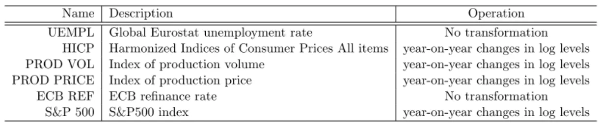
into account.The next table presents which variables I have used and what kind of operations I have applied before using them in the forecast exercise: The operations are mainly to insure
Name Description Operation
UEMPL Global Eurostat unemployment rate No transformation HICP Harmonized Indices of Consumer Prices All items year-on-year changes in log levels PROD VOL Index of production volume year-on-year changes in log levels PROD PRICE Index of production price year-on-year changes in log levels
ECB REF ECB refinance rate No transformation S&P 500 S&P500 index year-on-year changes in log levels
Table 2: Macro variables and their time series
the stationarity of the macro data and are in accordance with the specifications of de Pooter et al. (2007). All macro variables have been retrieved with Bloomberg for the period of December 1998 until February 2009.
Next up, the results of this report.
5
Results
The results of this work are vast and can best be evaluated with own experimentation of the Matlab GUI program. However, my goals in this section are twofold. Firstly, I want to show that all methods have been implemented correctly. Secondly, I want to demonstrate the forecast power of all of the implemented models in various situations.
5.1 Validation of the code
First up, the Nelson Siegel and the Random Walk. Next, the principal component forecast model.
5.1.1 Validation of the Nelson Siegel forecast model and the Random Walk
The easiest way to validated the implementation of the Nelson Siegel and the Random Walk forecast models, is by reproducing results as found in literature. I have chosen to compare my results with Diebold and Li (2006) because they also implement an AR(1) version of the Nelson Siegel model. As discussed before, identical results are not achievable due to a similar but different database.
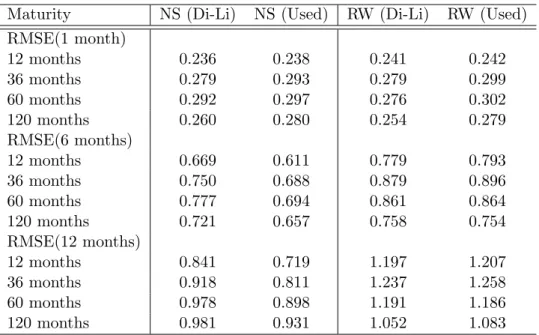
Table 3 lets us see the comparison between the forecasts of Diebold and Li (2006) and my forecasts. It presents the Root Mean Square out of sample forecast Errors (RMSE). Like Diebold and Li (2006) the U.S. Treasury yields are forecasted base on an in-sample history from January 1985 until January 1994 and an out-of-sample history from January 1985 until December 2000. Moreover, out-of-sample forecasts have been made for a 1 month, a 6 months and a 12 months horizon. The differences in RMSE of both implementations in table 3 are small and mainly caused by the fact that Diebold and Li used an unsmoothed dataset and that they have used more maturities. Moreover, for both implementations, the RMSE shows similar behavior when the maturity increases. For example, for a forecast horizon of 1 month, both NS (Di-Li) and NS (used) RMSE rises up to the maturity of 60 months and then starts falling. This table helps us to understand that:
Maturity NS (Di-Li) NS (Used) RW (Di-Li) RW (Used) RMSE(1 month)
12 months 0.236 0.238 0.241 0.242
36 months 0.279 0.293 0.279 0.299
60 months 0.292 0.297 0.276 0.302
120 months 0.260 0.280 0.254 0.279
RMSE(6 months)
12 months 0.669 0.611 0.779 0.793
36 months 0.750 0.688 0.879 0.896
60 months 0.777 0.694 0.861 0.864
120 months 0.721 0.657 0.758 0.754
RMSE(12 months)
12 months 0.841 0.719 1.197 1.207
36 months 0.918 0.811 1.237 1.258
60 months 0.978 0.898 1.191 1.186
120 months 0.981 0.931 1.052 1.083
Table 3: Comparison of the RMSE of out-of-sample forecasting of the U.S. Treasury Yields, over the period of January 1994 until December 2000. The data starts in January 1985, the AR is specified with 1 lag. INCREASING TIME WINDOW. ”Di-Li” stands for ”Diebold and Li” and ”Used” stands for ”used in this work”.
2. The Neslon Siegel model is implemented correctly
3. The recursive forecasting technique is implemented correctly
Next up, the verification of the principal component forecast model.
5.1.2 Validation of the principal component forecast model
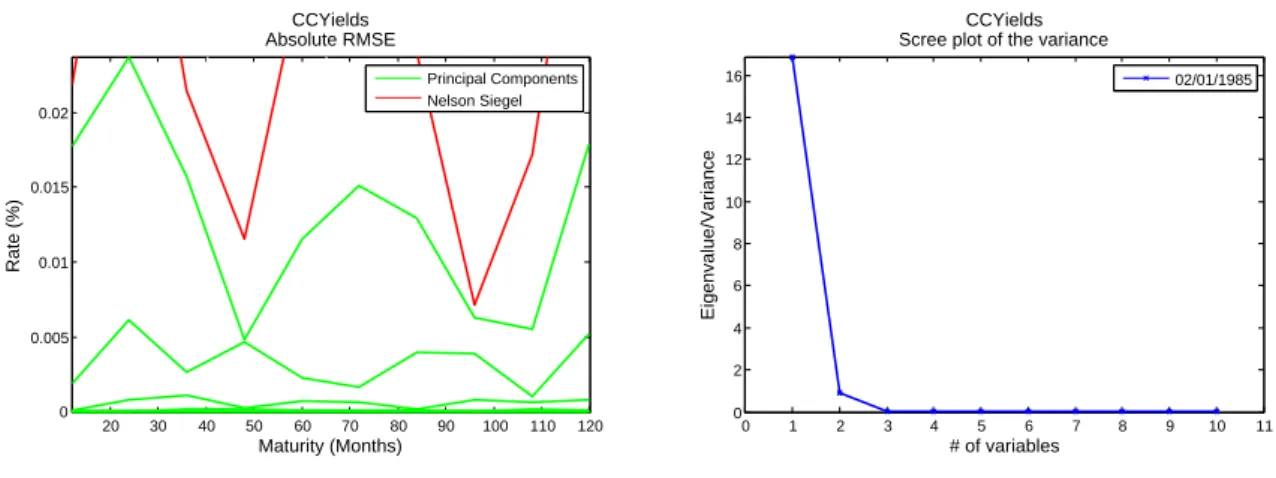
Testing if the principal component forecast model is correct is not so straightforward, mainly because the forecasts are series dependent. Let me explain this better. Imagine a database that is build with rates as interpolated by the Neslon Siegel three factor method. Now imagine applying the principal component method onto that database. Logically, a three factor Principal Component model fits all yields perfectly. Although, Nelson Siegel and the Principal Component each fit the yields perfectly, their timeseries are completely different. Remember, PC has standardized and independent timeseries. Timeseries for NS are not standardized and correlated. This means that an AR process will never forecast the same results.
20 30 40 50 60 70 80 90 100 110 120 0
0.005 0.01 0.015 0.02
CCYields Absolute RMSE
Maturity (Months)
Rate (%)
Principal Components Nelson Siegel
0 1 2 3 4 5 6 7 8 9 10 11
0 2 4 6 8 10 12 14 16
CCYields Scree plot of the variance
# of variables
Eigenvalue/Variance
02/01/1985
Figure 1: Left plot: RMSE of various principal component approximations (3 factors and more) and of a Nelson Siegel (λ= 0.0609) approximation of the U.S. Treasury Yield curve. Specifically, the first approximation was based on a history form 02/01/1985 until 03/05/1993, the consecutive approximations up to December 2000 were made with the rolling time window technique. Right plot: the scree plot of a principal component analysis of the U.S. Treasury Yield curve.
should be. Second, when increasing the number of components, the RMSE goes to zero for all maturities. More evidence is provided by the right plot. Namely, as expected, for yield curve data, three factors characterize almost all of the variance of the U.S. Treasury yield curve. From the third eigenvalue on, all eigenvalues are almost zero.
Based on the fact that I have proved that the recursive forecasting technique, the transition equation and the principal component method are implemented correctly, I assume that also the principal component forecast method is implemented correctly.
5.2 The Euro Interest Rate Swap curve
The statistics of the Euro Interest Rate Swap curve presented in table 4 are based on a history from 1999 until January 2009. Note that at a five percent level, we can not reject the hypothesis of having a unit root for all of the yields. This means that none of the timeseries of the yields are stationary and that all yields may follow a Random Walk process. Moreover, only β3,f2 and f3 seem not tho have a unit root.
5.3 Forecasting the Euro Interest Rate Swap curve
In order to investigate the forecastability of the Euro Internet Rate Swap curve, I have implemented 9 similar but yet different forecast models, which I have described in detail in the methodology section of this report. The Random Walk (RW), the Principal Component AR model (PC AR), the Principal Component model with AR of the differences (PC DAR), the differenced Principal Component AR model (DPC AR), the Principal Component model with Dickey Fuller (PC AR DF), the Principal Component Regression Model (PC REG), the Nelson Siegel AR forecast model (NS AR), the Nelson Siegel model with AR of the differences
3. In what follows next, I will compare these models for different set ups. Specifically, I can
Maturity Mean (%) Stdv(%) ρˆ(1) ADF Maturity Mean (%) Stdv(%) ρˆ(1) ADF 1 months 3.236 0.955 0.962 0.297 72 months 4.117 0.737 0.939 0.190 3 months 3.327 1.008 0.972 0.245 84 months 4.212 0.720 0.940 0.175 6 months 3.376 1.018 0.972 0.237 96 months 4.297 0.705 0.941 0.166 12 months 3.453 1.020 0.963 0.259 108 months 4.370 0.692 0.941 0.155 24 months 3.601 0.928 0.950 0.234 120 months 4.431 0.681 0.941 0.149 36 months 3.754 0.856 0.945 0.224 180 months 4.647 0.659 0.945 0.144 48 months 3.892 0.802 0.940 0.214 240 months 4.747 0.654 0.947 0.139 60 months 4.009 0.764 0.939 0.205 360 months 4.769 0.666 0.939 0.115
β1(NS) 4.957 0.689 0.951 0.098 f1 (PC) 0 1 0.958 0.127
β2(NS) -1.657 1.011 0.961 0.254 f2 (PC) 0 1 0.933 0.013
β3(NS) -1.489 1.616 0.877 0.060 f3 (PC) 0 1 0.864 0.004
Table 4: Mean, standard deviation and augmented Dickey Fuller test of the Euro Interest Rate Swap curve, its Nelson Siegel factors (β1,β2,β3) and its first three principal components
(f1,f2,f3). Note that fore the Euro Interest Rate Swap curve, the best Neslon Siegel fits were found fore λ= 0.0501. The ADF statistics denote the significance level accepting the hypothesis of having a unit root. The data ranges from December 1999 until January 2009.
change the forecast horizon, the number of factors, the number of lags, the history and the independent variables.
As we will see below, both the forecasting horizon and the history scheme play a very important role on the forecastability of the models. I will start the results by discussing the effect of the time transition scheme onto the out-of-sample RMSE.
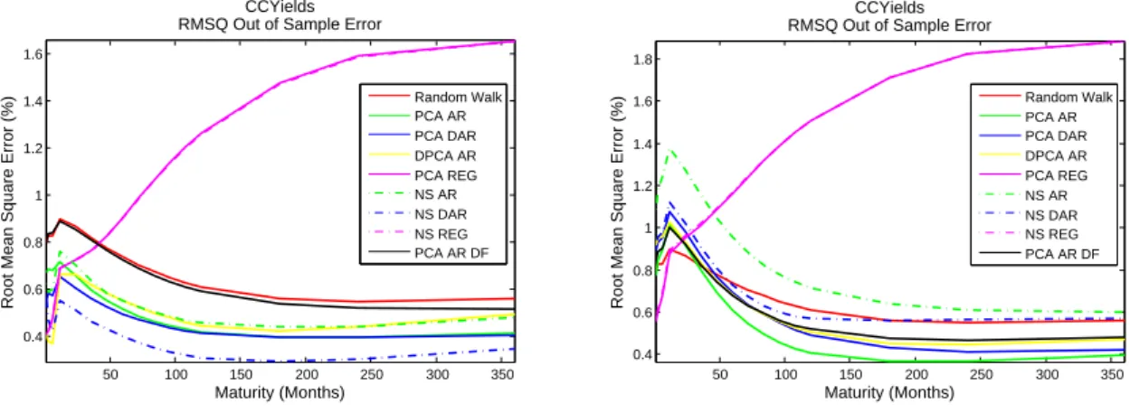
5.3.1 Rolling History vs. Increasing History
Rote that the difference will more easily noticeable when specifying a small in sample history as a start. The rolling history will slide a time window of a short length through time, while the increasing history will get bigger as time passes. Figure 2 demonstrates the effect on the out-of-sample RMSE when making a 12 month Euro Interest Rate Swamp forecast. Note
50 100 150 200 250 300 350
0.4 0.6 0.8 1 1.2 1.4 1.6
CCYields RMSQ Out of Sample Error
Maturity (Months)
Root Mean Square Error (%)
Random Walk PCA AR PCA DAR DPCA AR PCA REG NS AR NS DAR NS REG PCA AR DF
50 100 150 200 250 300 350
0.4 0.6 0.8 1 1.2 1.4 1.6 1.8
CCYields RMSQ Out of Sample Error
Maturity (Months)
Root Mean Square Error (%)
Random Walk PCA AR PCA DAR DPCA AR PCA REG NS AR NS DAR NS REG PCA AR DF
that the rolling time history has a huge advantage on the increasing time window. From an economical point of view this make sense. Economies and monetary policies change over time. Because the rolling time window has less memory, it is able to adapt much faster to economical deviations. As could be expected, the rolling time window is better for out-of-sample forecasting. For all results that follow next have been calculated with a rolling time window. Next up, the influences of the length of the rolling time window.
5.3.2 Influence of the length of the time window
The influence of the length of the time window can be measured by evaluating the out-of-sample accuracy for a short time window and a medium time window, for forecast horizons of 1 month, 6 months and 12 months. The short time window considers an initial in-sample time window from 31/12/1999 until 31/07/2002 (32 months) and the medium time window considers an initial in-sample time window from 31/12/1999 until 30/12/2005 (73 months). Their are 110 observations for each variable in the Euro Interest Rate Swap curve. 4 Tables 7, 8, 9, 10, 11, 13 contain information about the forecast RMSE and about the West and Clark (2006) statistics for nested models. A positive value of the West and Clark (2006) statistic in one of the table indicates a significant improvement in forecast accuracy compared to the random walk.
1 Month forecast horizon For a forecast horizon of 1 months, the Random Walk is the very difficult to beat due to the extremely high autocorrelations. Tables 7 and 8 demonstrate that changing the length of the history has little or no influence on the forecast behavior for each of the models. Note that although some of the models exhibit a lower RMSE than the RMSE of the Random walk for some maturities, the statistics in the lower table of tables 8 and 8 indicate that the difference is not statistically different from zero at a five percent level.
6 Month forecast horizon Tables 9 and 10 present the results of the 6 month ahead forecast exercise. This time, the results in table 9 are much better than the results in table 10. Moreover, models such as the PC AR, beat the random walk significantly for intermediate maturities. It is now clear that when forecasting 6 months ahead, a short history should be used. Based on this result we can preliminarily assume that for a 6 month ahead out-of-sample forecast exercise, shorter time windows yield better results.
12 Month forecast horizon Tables 11 and 13 present the results of the 12 month ahead forecast exercise. The time window effect is even more pronounced and the PC AR, PC DAR, NS AR and NS DAR model outperform the Random Walk for all maturities. In order to assure the reader that the time window effect is not curve specific, I have included evidence from the U.S. Treasury curve in the appendix. Compare tables 14 and 5 to see that a shorter time window would have improved the results of Diebold and Li (2006). Even in a newer data set the time window effect is still valid, see table 15 and 16. Again, the shortest time window yields the best results.
5.3.3 Influence of the number of included lags
As before, I have investigated the influence of the number of included lags for the three different forecast horizons.
1 Month forecast horizon I have investigated the effect of lags on short term forecast by running my Matlab GUI program for different history lengths and different lags. Unfortu-nately, lags do not improve the forecasts and none of the forecast models beats the random walk significantly.
6 Months forecast horizon The effect of lags on the models is diverse. I have tried lags from 1 to 12 and I have seen that for a specific model sometimes the estimation improves and other times the estimation worsens. I have not included results in this report, but it can easily be simulated with my Matlab GUI program.
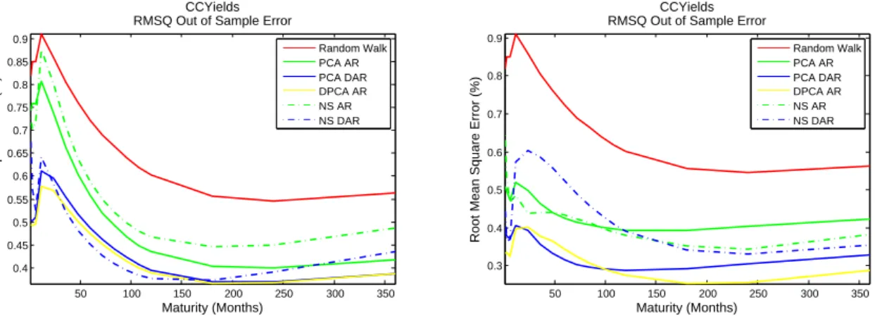
12 Months forecast horizon When forecasting 12 months ahead, lags can be useful in combination with a short time window. Figure 3 illustrates the effect of including 10 lags in the AR process on the forecast. As can be seen, the mean square errors of the models drop
50 100 150 200 250 300 350
0.4 0.45 0.5 0.55 0.6 0.65 0.7 0.75 0.8 0.85 0.9
CCYields RMSQ Out of Sample Error
Maturity (Months)
Root Mean Square Error (%)
Random Walk PCA AR PCA DAR DPCA AR NS AR NS DAR
50 100 150 200 250 300 350
0.3 0.4 0.5 0.6 0.7 0.8 0.9
CCYields RMSQ Out of Sample Error
Maturity (Months)
Root Mean Square Error (%)
Random Walk PCA AR PCA DAR DPCA AR NS AR NS DAR
Figure 3: Left plot: the RMSE of principal component approximations (3 factors and more) and of a Nelson Siegel approximation of the U.S. Treasury Yield curve. Specifically, the first approximations were based on a history form 02/01/1985 until 03/05/1993, the consecutive approximations up to December 2000 were made with the rolling timewindow technique. Right plot: the scree plot of a principal component analysis of the U.S. Treasury Yield curve. Figures based on monthly U.S. Treasury data from 02/01/1985 until 05/03/1993
reasonably. However, the improvement when using lags is not consistent. The effect of lags on factor series is thus not useful.
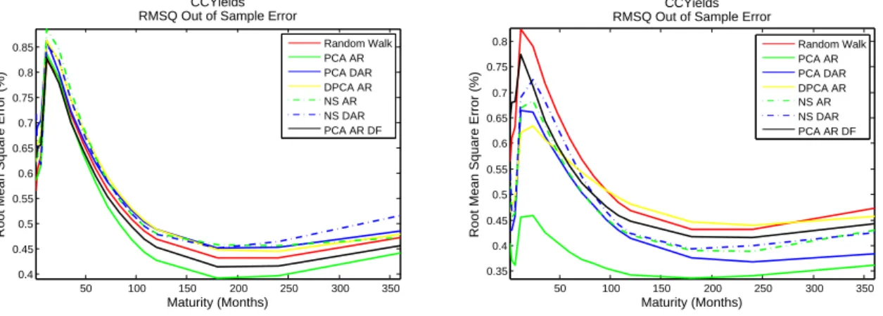
5.3.4 The effect of Macro Factors
1 Month forecast horizon When experimenting with Macro Factors and lagged Macro factors for different time windows, macro factors did not seem to improve the 1 Month forecast results.
6 Month forecast horizon The macro factors have a positive effect on the forecastability of the implemented models, no matter the length of the time window. Estimations with a longer time window now sometimes give better estimations than when calculating with a shorter time window. The macro effect can be seen quite well when comparing the two plots in figure 4. Note that including a small number lags of the macro variables (up to 5) reduces
50 100 150 200 250 300 350
0.4 0.45 0.5 0.55 0.6 0.65 0.7 0.75 0.8 0.85
CCYields RMSQ Out of Sample Error
Maturity (Months)
Root Mean Square Error (%)
Random Walk PCA AR PCA DAR DPCA AR NS AR NS DAR PCA AR DF
50 100 150 200 250 300 350
0.35 0.4 0.45 0.5 0.55 0.6 0.65 0.7 0.75 0.8
CCYields RMSQ Out of Sample Error
Maturity (Months)
Root Mean Square Error (%)
Random Walk PCA AR PCA DAR DPCA AR NS AR NS DAR PCA AR DF
Figure 4: Left plot: the RMSE forecast error for various forecast methods without macro factors. Right plot: the RMSE forecast error for various forecast methods with 3 macro factors and 1 lag. The data were calculated for an in sample history of 30/01/04 scree plot of a principal component analysis of the U.S. Treasury Yield curve. Figures based on monthly U.S. Treasury data from 02/01/1985 until 05/03/1993
the error even more.
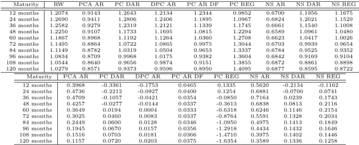
12 Month forecast horizon Similar effects are noticeable for a forecast horizon of 12 months. Including macro factors also reduces the forecast error. Eventhough the RMSE in table 11 is already significantly lower for PC AR, PD DAR, NS AR and NS DAR compared to the RMSE of the Random Walk, table 12 illustrates that adding two macro factors reduce the RMSE even more.
6
Conclusion
I have implemented four macro factor augmented dynamic versions of the principal component method in order to make an out-of-sample forecast exercise of the Euro Interest Rate Swap Curve. Moreover, I have implemented three Nelson-Siegel forecast models and the Random Walk. After having studied a lot of different forecast results we can remember the following:
2. When using a big forecast step and a small rolling time window, we can significantly outperform the Random Walk with a series of methods.
3. Incorporating Macro factors improves the results.
In relation with choice of forecast model, I have noticed that the results depend a lot on the constraints. On average, I believe that for three factors, the Principal Component models are a bit more accurate than the Neslon Siegel models. Moreover, Principal Component models do not put any artificial restriction onto the data. This flexibility makes this method general and also applicable on other data types, such as the macro variables. Compared to the Nelson Siegel model, the Principal Component Model does have the disadvantage of recomputing its factors at each point in time. This not only increases the difficulty of implementation, but also the computational effort. Another downside is the fact that at maturities other than the observed, interpolation tactics must be used.
References
Ang, A., Piazzesi, M., A no-arbitrage vector autoregression of term structure dynamics with macroeconomic and latent variables, Journal of Monetary Economics, volume 50(4), (2003), pp. 745–787, URLhttp://dx.doi.org/10.1016/S0304-3932(03)00032-1.
Bauer, M.D., Dahl, G., Forecasting the Term Structure using Nelson-Siegel Factors and Com-bined Forecasts, Technical report, UC San Diego Economics (2007).
Blaskowitz, O., Herwatz, H., Adaptive Forecasting of the EURIBOR Swap Term Struc-ture, SFB 649 Discussion Papers SFB649DP2008-017, Sonderforschungsbereich 649, Hum-boldt University, Berlin, Germany (2008), URLhttp://ideas.repec.org/p/hum/wpaper/ sfb649dp2008-017.html.
Bliss, R.R., Movements in the term structure of interest rates, Economic Review, (Q 4), (1997), pp. 16–33, URL http://ideas.repec.org/a/fip/fedaer/y1997iq4p16-33nv. 82no.4.html.
Christensen, J.H.E., Diebold, F.X., Rudebusch, G.D., An arbitrage-free generalized Nelson-Siegel term structure model, Technical report (2008).
Diebold, F.X., Li, C., Forecasting the term structure of government bond yields, Journal of Econometrics, volume 130(2), (2006), pp. 337–364, URLhttp://ideas.repec.org/a/ eee/econom/v130y2006i2p337-364.html.
Diebold, F.X., Rudebusch, G.D., Aruoba, S.B., The Macroeconomy and the Yield Curve: A Dynamic Latent Factor Approach, NBER Working Papers 10616, National Bureau of Economic Research, Inc (2004), URL http://ideas.repec.org/p/nbr/nberwo/10616. html.
Duffee, G.R., Term Premia and Interest Rate Forecasts in Affine Models, Journal of Fi-nance, volume 57(1), (2002), pp. 405–443, URLhttp://ideas.repec.org/a/bla/jfinan/ v57y2002i1p405-443.html.
Duffee, G.R., Forecasting with the term structure: The role of no-arbitrage (2008).
Exterkate, P., Forecasting the Yield Curve in a Data-Rich Environment (2008).
Field, A., Discovering Statistics Using SPSS (Introducing Statistical Methods series), Sage Publications Ltd, third edition edition (2009), URL http://www.amazon.ca/exec/ obidos/redirect?tag=citeulike09-20\&path=ASIN/1847879071.
Gurkaynak, R.S., Sack, B., Wright, J.H., The U.S. Treasury yield curve: 1961 to the present, Journal of Monetary Economics, volume 54(8), (2007), pp. 2291–2304, URLhttp://ideas. repec.org/a/eee/moneco/v54y2007i8p2291-2304.html.
de Pooter, M.D., Ravazzolo, F., van Dijk, D., Predicting the Term Structure of Interest Rates: Incorporating Parameter Uncertainty, Model Uncertainty and Macroeconomic Information, Tinbergen Institute Discussion Papers 07-028/4, Tinbergen Institute (2007), URL http: //ideas.repec.org/p/dgr/uvatin/20070028.html.
Remolona, E.M., Wooldridge, P.D., The euro interest rate swap market (2003).
A
Forecast Result Tables
Maturity RW PCA AR PC DAR DPC AR PC AR DF PC REG NS AR NS DAR NS REG 12 months 1.2074 0.9143 1.2643 1.2134 1.2344 0.9852 0.6700 1.1956 1.1675 24 months 1.2690 0.9411 1.2806 1.2406 1.1895 1.0967 0.6824 1.2021 1.1529 36 months 1.2582 0.9279 1.2319 1.2121 1.1339 1.1745 0.6661 1.1540 1.1008 48 months 1.2250 0.9107 1.1733 1.1695 1.0815 1.2294 0.6589 1.0961 1.0480 60 months 1.1867 0.8968 1.1192 1.1264 1.0360 1.2708 0.6623 1.0417 1.0026 72 months 1.1495 0.8864 1.0722 1.0865 0.9975 1.3044 0.6703 0.9939 0.9654 84 months 1.1149 0.8782 1.0319 1.0504 0.9653 1.3337 0.6784 0.9525 0.9352 96 months 1.0834 0.8709 0.9968 1.0175 0.9382 1.3604 0.6842 0.9169 0.9104 108 months 1.0544 0.8640 0.9656 0.9874 0.9151 1.3855 0.6872 0.8861 0.8898 120 months 1.0279 0.8571 0.9373 0.9596 0.8950 1.4095 0.6877 0.8595 0.8722
Maturity PCA AR PC DAR DPC AR PC AR DF PC REG NS AR NS DAR NS REG 12 months 0.3968 -0.3361 -0.1753 0.0465 0.1335 0.5620 -0.2134 -0.1162 24 months 0.4736 -0.2212 -0.0927 0.0400 0.1254 0.6881 -0.0700 0.0741 36 months 0.4709 -0.1057 -0.0421 0.0354 -0.0850 0.7164 0.0239 0.1743 48 months 0.4257 -0.0277 -0.0144 0.0337 -0.3613 0.6838 0.0813 0.2116 60 months 0.3649 0.0194 0.0004 0.0333 -0.6318 0.6246 0.1146 0.2154 72 months 0.3025 0.0460 0.0083 0.0337 -0.8764 0.5591 0.1328 0.2034 84 months 0.2449 0.0600 0.0128 0.0346 -1.0950 0.4975 0.1413 0.1849 96 months 0.1945 0.0670 0.0157 0.0356 -1.2918 0.4434 0.1432 0.1646 108 months 0.1516 0.0703 0.0181 0.0366 -1.4710 0.3975 0.1402 0.1446 120 months 0.1157 0.0720 0.0203 0.0375 -1.6354 0.3589 0.1336 0.1258
Table 5: Upper Table: Comparison of out-of-sample forecasts for all implemented methods for the U.S. Treasury curve. This setup is similar to the Diebold and Li (2006) setup. Forecast horizon of 12 months. In sample history from 02/01/1985 until 02/01/1994 and out of sample domain from 02/01/1994 until 02/12/2006. ROLLING TIME WINDOW. 3 factors are used for the PC models. The AR model is specified with 1 lag. Lower Table: West and Clark (2006) statistic of the results. Positive numbers show that the forecasts are significantly better that the Random Walk forecasts at a 5% tolerance.
Maturity RW PCA AR PC DAR DPC AR PC AR DF PC REG NS AR NS DAR NS REG 12 months 1.2074 0.7918 1.2863 1.2633 0.8995 0.9336 0.7212 1.2628 0.9308 24 months 1.2690 0.8726 1.2971 1.2744 0.9367 1.0714 0.7645 1.2611 1.0696 36 months 1.2582 0.9037 1.2510 1.2368 0.9391 1.1576 0.7988 1.2036 1.1563 48 months 1.2250 0.9198 1.1940 1.1869 0.9328 1.2168 0.8338 1.1380 1.2159 60 months 1.1867 0.9303 1.1392 1.1374 0.9252 1.2619 0.8646 1.0772 1.2613 72 months 1.1495 0.9373 1.0901 1.0923 0.9177 1.2994 0.8873 1.0240 1.2990 84 months 1.1149 0.9413 1.0472 1.0523 0.9103 1.3328 0.9009 0.9777 1.3326 96 months 1.0834 0.9426 1.0099 1.0168 0.9026 1.3636 0.9062 0.9375 1.3636 108 months 1.0544 0.9414 0.9774 0.9853 0.8944 1.3928 0.9050 0.9024 1.3930 120 months 1.0279 0.9384 0.9492 0.9570 0.8859 1.4205 0.8990 0.8715 1.4209
Maturity PCA AR PC DAR DPC AR PC AR DF PC REG NS AR NS DAR NS REG 12 months 0.4709 -0.3444 -0.2609 0.2760 0.2926 0.4654 -0.3439 0.2988 24 months 0.4944 -0.2444 -0.1558 0.3729 0.2557 0.5507 -0.1736 0.2587 36 months 0.4377 -0.1506 -0.0966 0.3689 0.0119 0.5027 -0.0454 0.0127 48 months 0.3491 -0.0820 -0.0593 0.3240 -0.2974 0.3991 0.0378 -0.2973 60 months 0.2559 -0.0333 -0.0334 0.2678 -0.5916 0.2873 0.0896 -0.5920 72 months 0.1701 0.0006 -0.0147 0.2130 -0.8552 0.1889 0.1217 -0.8561 84 months 0.0963 0.0235 -0.0012 0.1644 -1.0906 0.1113 0.1415 -1.0919 96 months 0.0352 0.0379 0.0085 0.1232 -1.3029 0.0544 0.1529 -1.3047 108 months -0.0143 0.0458 0.0150 0.0891 -1.4964 0.0150 0.1584 -1.4987 120 months -0.0539 0.0486 0.0192 0.0614 -1.6739 -0.0110 0.1593 -1.6767
Maturity RW PC AR PC DAR DPC AR PC AR DF PC REG NS AR NS DAR NS REG 1 months 0.2318 0.2417 0.2048 0.2098 0.2412 0.1721 0.3022 0.2699 0.1741 3 months 0.2125 0.2110 0.1654 0.1935 0.2124 0.1835 0.2034 0.1470 0.1843 6 months 0.2117 0.2048 0.1536 0.1918 0.2037 0.2462 0.1937 0.1274 0.2457 12 months 0.2231 0.2729 0.2260 0.1962 0.2643 0.5100 0.3976 0.3183 0.5069 24 months 0.2382 0.2650 0.2350 0.2210 0.2600 0.6082 0.3466 0.2811 0.6051 36 months 0.2302 0.2388 0.2177 0.2172 0.2366 0.7033 0.2865 0.2406 0.7008 48 months 0.2233 0.2245 0.2086 0.2128 0.2237 0.8160 0.2531 0.2245 0.8142 60 months 0.2115 0.2090 0.1970 0.2029 0.2089 0.9247 0.2314 0.2098 0.9233 72 months 0.1998 0.1960 0.1866 0.1924 0.1962 1.0277 0.2144 0.1963 1.0266 84 months 0.1895 0.1861 0.1779 0.1829 0.1861 1.1222 0.2001 0.1844 1.1214 96 months 0.1801 0.1781 0.1711 0.1743 0.1778 1.2080 0.1887 0.1734 1.2074 108 months 0.1733 0.1724 0.1666 0.1683 0.1715 1.2827 0.1798 0.1644 1.2822 120 months 0.1677 0.1673 0.1619 0.1630 0.1660 1.3471 0.1733 0.1563 1.3467 180 months 0.1513 0.1600 0.1553 0.1498 0.1560 1.5741 0.1730 0.1538 1.5739 240 months 0.1437 0.1663 0.1595 0.1443 0.1603 1.6945 0.1884 0.1687 1.6944 360 months 0.1495 0.1936 0.1819 0.1510 0.1865 1.7592 0.2438 0.2213 1.7592
Maturity PCA AR PC DAR DPC AR PC AR DF PC REG NS AR NS DAR NS REG 1 months -0.0162 -0.0068 -0.0082 -0.0141 0.0022 -0.0724 -0.0543 0.0031 3 months -0.0060 -0.0063 -0.0079 -0.0057 -0.0210 -0.0080 0.0006 -0.0211 6 months -0.0049 -0.0006 -0.0066 -0.0035 -0.0520 -0.0153 0.0005 -0.0519 12 months -0.0443 -0.0114 -0.0027 -0.0361 -0.2881 -0.1633 -0.0887 -0.2825 24 months -0.0252 -0.0108 -0.0022 -0.0212 -0.4084 -0.0956 -0.0375 -0.4016 36 months -0.0103 -0.0037 -0.0024 -0.0080 -0.5493 -0.0449 -0.0158 -0.5438 48 months -0.0046 -0.0015 -0.0028 -0.0032 -0.7561 -0.0241 -0.0125 -0.7524 60 months -0.0024 -0.0013 -0.0029 -0.0016 -0.9907 -0.0167 -0.0107 -0.9880 72 months -0.0017 -0.0016 -0.0030 -0.0012 -1.2393 -0.0128 -0.0092 -1.2375 84 months -0.0018 -0.0020 -0.0030 -0.0013 -1.4897 -0.0099 -0.0079 -1.4886 96 months -0.0022 -0.0026 -0.0030 -0.0016 -1.7328 -0.0083 -0.0064 -1.7322 108 months -0.0025 -0.0029 -0.0030 -0.0017 -1.9575 -0.0071 -0.0048 -1.9573 120 months -0.0027 -0.0029 -0.0029 -0.0018 -2.1602 -0.0067 -0.0034 -2.1603 180 months -0.0057 -0.0052 -0.0035 -0.0036 -2.9492 -0.0131 -0.0062 -2.9501 240 months -0.0117 -0.0095 -0.0038 -0.0089 -3.4204 -0.0225 -0.0132 -3.4219 360 months -0.0267 -0.0205 -0.0046 -0.0234 -3.6963 -0.0615 -0.0484 -3.6988
Table 7: Upper Table: Comparison of out-of-sample forecasts for all implemented methods for the Euro Interest Rate Swap curve. Forecast horizon of 1 month. In sample history from 31/12/1999 until 31/07/2002 and out of sample domain from 31/07/2002 until 29/01/2009. ROLLING TIME WINDOW. 3 factors are used for the PC models. The AR model is specified with 1 lag. Lower Table:West and Clark (2006) statistic of the results. Positive numbers show that the forecasts are significantly better that the Random Walk forecasts at a 5% tolerance.
Maturity RW PCA AR PC DAR DPC AR PC AR DF PC REG NS AR NS DAR NS REG 1 months 0.3189 0.3144 0.2723 0.2984 0.3167 0.2582 0.3953 0.3584 0.2496 3 months 0.2889 0.2738 0.2132 0.2586 0.2747 0.2387 0.2426 0.2019 0.2350 6 months 0.2840 0.2513 0.1877 0.2537 0.2501 0.3043 0.2307 0.1915 0.3032 12 months 0.2795 0.3789 0.3088 0.2585 0.3647 0.6441 0.5018 0.4484 0.6362 24 months 0.2748 0.3282 0.2755 0.2571 0.3121 0.6853 0.4097 0.3578 0.6780 36 months 0.2555 0.2752 0.2379 0.2397 0.2603 0.6712 0.3148 0.2758 0.6652 48 months 0.2389 0.2441 0.2157 0.2240 0.2314 0.6638 0.2596 0.2326 0.6589 60 months 0.2222 0.2206 0.1986 0.2086 0.2101 0.6654 0.2264 0.2082 0.6615 72 months 0.2086 0.2027 0.1853 0.1966 0.1944 0.6728 0.2041 0.1912 0.6698 84 months 0.1968 0.1897 0.1758 0.1862 0.1832 0.6852 0.1879 0.1781 0.6830 96 months 0.1882 0.1808 0.1682 0.1791 0.1757 0.7035 0.1768 0.1681 0.7020 108 months 0.1805 0.1733 0.1625 0.1727 0.1693 0.7232 0.1674 0.1599 0.7223 120 months 0.1762 0.1695 0.1590 0.1694 0.1665 0.7453 0.1637 0.1560 0.7449 180 months 0.1616 0.1645 0.1547 0.1586 0.1633 0.8475 0.1807 0.1759 0.8482 240 months 0.1551 0.1811 0.1694 0.1538 0.1810 0.8983 0.2079 0.2041 0.8987 360 months 0.1695 0.2441 0.2295 0.1688 0.2441 0.9077 0.2850 0.2814 0.9066
Maturity PCA AR PC DAR DPC AR PC AR DF PC REG NS AR NS DAR NS REG 1 months -0.0145 -0.0015 -0.0245 -0.0145 0.0057 -0.1086 -0.0790 0.0067 3 months -0.0079 -0.0043 -0.0153 -0.0070 -0.0318 -0.0014 -0.0021 -0.0324 6 months -0.0080 -0.0027 -0.0141 -0.0059 -0.0793 -0.0236 -0.0166 -0.0809 12 months -0.1115 -0.0322 -0.0051 -0.0987 -0.4858 -0.2689 -0.1960 -0.4649 24 months -0.0557 -0.0191 -0.0039 -0.0410 -0.5656 -0.1413 -0.0831 -0.5455 36 months -0.0191 -0.0043 -0.0032 -0.0095 -0.5395 -0.0516 -0.0216 -0.5244 48 months -0.0079 -0.0015 -0.0024 -0.0022 -0.5309 -0.0184 -0.0079 -0.5200 60 months -0.0048 -0.0018 -0.0020 -0.0011 -0.5424 -0.0077 -0.0056 -0.5346 72 months -0.0034 -0.0023 -0.0018 -0.0008 -0.5634 -0.0036 -0.0047 -0.5583 84 months -0.0029 -0.0031 -0.0016 -0.0010 -0.5929 -0.0019 -0.0044 -0.5900 96 months -0.0023 -0.0029 -0.0016 -0.0007 -0.6320 -0.0010 -0.0036 -0.6307 108 months -0.0021 -0.0026 -0.0015 -0.0005 -0.6743 -0.0009 -0.0028 -0.6745 120 months -0.0022 -0.0023 -0.0015 -0.0005 -0.7198 -0.0021 -0.0030 -0.7210 180 months -0.0043 -0.0016 -0.0022 -0.0038 -0.9384 -0.0162 -0.0145 -0.9421 240 months -0.0172 -0.0111 -0.0022 -0.0192 -1.0561 -0.0300 -0.0275 -1.0596 360 months -0.0598 -0.0495 -0.0025 -0.0626 -1.0797 -0.0967 -0.0931 -1.0797
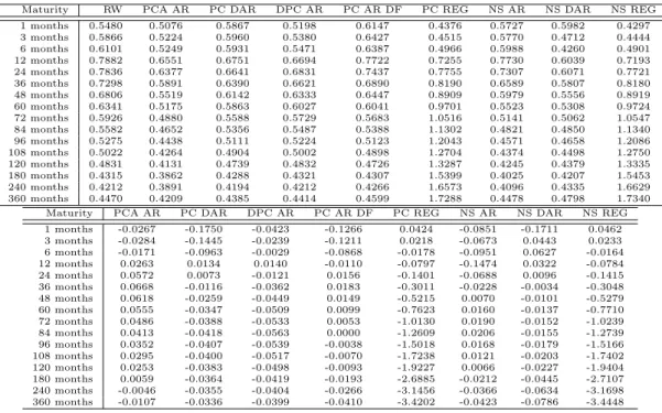
Maturity RW PCA AR PC DAR DPC AR PC AR DF PC REG NS AR NS DAR NS REG 1 months 0.5480 0.5076 0.5867 0.5198 0.6147 0.4376 0.5727 0.5982 0.4297 3 months 0.5866 0.5224 0.5960 0.5380 0.6427 0.4515 0.5770 0.4712 0.4444 6 months 0.6101 0.5249 0.5931 0.5471 0.6387 0.4966 0.5988 0.4260 0.4901 12 months 0.7882 0.6551 0.6751 0.6694 0.7722 0.7255 0.7730 0.6039 0.7193 24 months 0.7836 0.6377 0.6641 0.6831 0.7437 0.7755 0.7307 0.6071 0.7721 36 months 0.7298 0.5891 0.6390 0.6621 0.6890 0.8190 0.6589 0.5807 0.8180 48 months 0.6806 0.5519 0.6142 0.6333 0.6447 0.8909 0.5979 0.5556 0.8919 60 months 0.6341 0.5175 0.5863 0.6027 0.6041 0.9701 0.5523 0.5308 0.9724 72 months 0.5926 0.4880 0.5588 0.5729 0.5683 1.0516 0.5141 0.5062 1.0547 84 months 0.5582 0.4652 0.5356 0.5487 0.5388 1.1302 0.4821 0.4850 1.1340 96 months 0.5275 0.4438 0.5111 0.5224 0.5123 1.2043 0.4571 0.4658 1.2086 108 months 0.5022 0.4264 0.4904 0.5002 0.4898 1.2704 0.4374 0.4498 1.2750 120 months 0.4831 0.4131 0.4739 0.4832 0.4726 1.3287 0.4245 0.4379 1.3335 180 months 0.4315 0.3862 0.4288 0.4321 0.4307 1.5399 0.4025 0.4207 1.5453 240 months 0.4212 0.3891 0.4194 0.4212 0.4266 1.6573 0.4096 0.4335 1.6629 360 months 0.4470 0.4209 0.4385 0.4414 0.4599 1.7288 0.4478 0.4798 1.7340
Maturity PCA AR PC DAR DPC AR PC AR DF PC REG NS AR NS DAR NS REG 1 months -0.0267 -0.1750 -0.0423 -0.1266 0.0424 -0.0851 -0.1711 0.0462 3 months -0.0284 -0.1445 -0.0239 -0.1211 0.0218 -0.0673 0.0443 0.0233 6 months -0.0171 -0.0963 -0.0029 -0.0868 -0.0178 -0.0951 0.0627 -0.0164 12 months 0.0263 0.0134 0.0140 -0.0110 -0.0797 -0.1474 0.0322 -0.0784 24 months 0.0572 0.0073 -0.0121 0.0156 -0.1401 -0.0688 0.0096 -0.1415 36 months 0.0668 -0.0116 -0.0362 0.0183 -0.3011 -0.0228 -0.0034 -0.3048 48 months 0.0618 -0.0259 -0.0449 0.0149 -0.5215 0.0070 -0.0101 -0.5279 60 months 0.0555 -0.0347 -0.0509 0.0099 -0.7623 0.0160 -0.0137 -0.7710 72 months 0.0486 -0.0388 -0.0533 0.0053 -1.0130 0.0190 -0.0152 -1.0239 84 months 0.0413 -0.0418 -0.0563 0.0000 -1.2609 0.0206 -0.0155 -1.2739 96 months 0.0352 -0.0407 -0.0539 -0.0038 -1.5018 0.0168 -0.0179 -1.5166 108 months 0.0295 -0.0400 -0.0517 -0.0070 -1.7238 0.0121 -0.0203 -1.7402 120 months 0.0253 -0.0383 -0.0498 -0.0093 -1.9227 0.0066 -0.0227 -1.9404 180 months 0.0059 -0.0364 -0.0419 -0.0193 -2.6885 -0.0212 -0.0445 -2.7107 240 months -0.0046 -0.0355 -0.0404 -0.0266 -3.1456 -0.0366 -0.0634 -3.1698 360 months -0.0107 -0.0336 -0.0399 -0.0410 -3.4202 -0.0423 -0.0786 -3.4448
Table 9: Upper Table: Comparison of out-of-sample forecasts for all implemented methods for the Euro Interest Rate Swap curve. Forecast horizon of 6 months. In sample history from 31/12/1999 until 31/07/2002 and out of sample domain from 31/07/2002 until 29/01/2009. ROLLING TIME WINDOW. 3 factors are used for the PC models. The AR model is specified with 1 lag. Lower Table: West and Clark (2006) statistic of the results. Positive numbers show that the forecasts are significantly better that the Random Walk forecasts at a 5% tolerance.
Maturity RW PCA AR PC DAR DPC AR PC AR DF PC REG NS AR NS DAR NS REG 1 months 0.6987 0.7649 0.8203 0.7641 0.7176 0.6735 0.8751 0.8166 0.6753 3 months 0.7549 0.8303 0.8475 0.8143 0.7668 0.6799 0.8822 0.7605 0.6841 6 months 0.7796 0.8603 0.8698 0.8390 0.7939 0.7207 0.9451 0.7679 0.7256 12 months 1.0100 1.1308 1.0937 1.0707 1.0439 1.0090 1.2287 1.0258 1.0114 24 months 0.9602 1.0431 1.0281 1.0273 0.9821 1.0104 1.1781 0.9657 1.0122 36 months 0.8617 0.9176 0.9290 0.9340 0.8775 0.9660 1.0626 0.8628 0.9681 48 months 0.7828 0.8176 0.8528 0.8586 0.7960 0.9366 0.9581 0.7806 0.9391 60 months 0.7148 0.7326 0.7854 0.7933 0.7236 0.9163 0.8685 0.7145 0.9192 72 months 0.6567 0.6605 0.7269 0.7375 0.6605 0.9041 0.7943 0.6598 0.9074 84 months 0.6078 0.6020 0.6788 0.6907 0.6085 0.8983 0.7340 0.6148 0.9020 96 months 0.5691 0.5552 0.6374 0.6524 0.5651 0.9010 0.6883 0.5810 0.9050 108 months 0.5365 0.5172 0.6027 0.6201 0.5291 0.9070 0.6516 0.5529 0.9114 120 months 0.5140 0.4910 0.5773 0.5967 0.5035 0.9189 0.6262 0.5354 0.9236 180 months 0.4561 0.4284 0.5118 0.5355 0.4389 0.9873 0.5702 0.5107 0.9927 240 months 0.4537 0.4271 0.5012 0.5243 0.4354 1.0353 0.5608 0.5271 1.0408 360 months 0.5106 0.4835 0.5392 0.5600 0.4925 1.0735 0.5743 0.5715 1.0784
Maturity PCA AR PC DAR DPC AR PC AR DF PC REG NS AR NS DAR NS REG 1 months -0.1809 -0.3594 -0.1670 -0.1017 -0.1181 -0.4617 -0.3957 -0.1199 3 months -0.2255 -0.2917 -0.1833 -0.0782 -0.0004 -0.3165 -0.0614 -0.0073 6 months -0.2587 -0.2721 -0.1961 -0.0868 -0.0647 -0.4631 -0.0917 -0.0729 12 months -0.3963 -0.3002 -0.2298 -0.1316 -0.1690 -0.8235 -0.2374 -0.1770 24 months -0.2813 -0.2358 -0.2244 -0.1198 -0.2153 -0.7834 -0.1923 -0.2228 36 months -0.1911 -0.2111 -0.2092 -0.0923 -0.3007 -0.6530 -0.1533 -0.3089 48 months -0.1289 -0.1948 -0.1957 -0.0705 -0.3819 -0.5225 -0.1220 -0.3908 60 months -0.0856 -0.1765 -0.1841 -0.0500 -0.4614 -0.4210 -0.1029 -0.4710 72 months -0.0553 -0.1588 -0.1743 -0.0328 -0.5365 -0.3486 -0.0897 -0.5470 84 months -0.0374 -0.1456 -0.1665 -0.0222 -0.6051 -0.2981 -0.0799 -0.6164 96 months -0.0259 -0.1305 -0.1579 -0.0131 -0.6742 -0.2663 -0.0767 -0.6862 108 months -0.0202 -0.1192 -0.1506 -0.0083 -0.7381 -0.2453 -0.0769 -0.7509 120 months -0.0171 -0.1096 -0.1440 -0.0058 -0.7996 -0.2321 -0.0806 -0.8131 180 months -0.0171 -0.0900 -0.1264 -0.0054 -1.0487 -0.2164 -0.1209 -1.0646 240 months -0.0197 -0.0809 -0.1162 -0.0109 -1.1829 -0.2057 -0.1467 -1.1997 360 months -0.0191 -0.0703 -0.1037 -0.0186 -1.2271 -0.1522 -0.1352 -1.2433