Suppressing Fermi acceleration in two-dimensional driven billiards
Edson D. Leonel1,2and Leonid A. Bunimovich2 1
Departamento de Estatística, Matemática Aplicada e Computação—IGCE—UNESP—Univ Estadual Paulista, Avenida 24A, 1515 Bela Vista, CEP 13506-700—Rio Claro, SP, Brazil
2
School of Mathematics, Georgia Institute of Technology, Atlanta, Georgia 30332-0160, USA 共Received 3 December 2009; published 2 July 2010; corrected 7 July 2010兲
We consider a dissipative oval-like shaped billiard with a periodically moving boundary. The dissipation considered is proportional to a power of the velocityVof the particle. The three specific types of power laws used are:共i兲F⬀−V;共ii兲F⬀−V2and共iii兲F⬀−V␦with 1⬍␦⬍2. In the course of the dynamics of the particle,
if a large initial velocity is considered, case 共i兲 shows that the decay of the particle’s velocity is a linear function of the number of collisions with the boundary. For case共ii兲, an exponential decay is observed, and for 1⬍␦⬍2, an powerlike decay is observed. Scaling laws were used to characterize a phase transition from limited to unlimited energy gain for cases共ii兲and共iii兲. The critical exponents obtained for the phase transition in the case 共ii兲are the same as those obtained for the dissipative bouncer model. Therefore near this phase transition, these two rather different models belong to the same class of universality. For all types of dissipa-tion, the results obtained allow us to conclude that suppression of the unlimited energy growth is indeed observed.
DOI:10.1103/PhysRevE.82.016202 PACS number共s兲: 05.45.Pq, 05.45.Tp
I. INTRODUCTION
The systems where particles do not interact with each other and move freely experiencing elastic collisions from the boundary are called billiards 关1兴. Billiard type systems demonstrate regular关1兴, mixed 关2兴or fully chaotic behavior 关3兴, and are used in many physical experiments including reflection of light from mirrors关4兴, superconducting关5兴and confinement of electrons in semiconductors by electric po-tentials关6,7兴, waveguides关8,9兴, microwave billiards关10,11兴, ultracold atoms trapped in a laser potential关12–15兴and also mesoscopic quantum dots关16兴.
The famous phenomenon of Fermi acceleration共FA兲 关17兴 was studied in various billiardlike models关18–23兴where the boundary moves in time, i.e., it is time dependent. The intro-duction of time dependence into the boundary yields the par-ticle to change energy upon collision. If the collision is head-on/tail-on then the particle gains/loses energy. A key question addressed in studies on FA关17兴is whether a particle’s energy can grow to infinity. The answer to this question is not trivial and depends on the geometry of the boundary and the kind of time perturbation. The Loskutov-Ryabov-Akinshin 共LRA兲 conjecture关24兴claims that if the dynamics of the particle is chaotic while the boundary is static, thus this is a sufficient condition to observe FA when a time perturbation to the boundary is introduced. It has been shown recently关25兴that a time-dependent elliptic billiard can also generate FA, there-fore, the answer could also be “yes” even for共some兲 inte-grable billiards.
In this paper, we are concerned with the mechanisms of suppressing FA. We therefore study the dynamics of an en-semble of non interacting particles in a time-dependent oval-like shaped billiard. It is assumed that the particles experi-ence a drag force which is proportional to a power of the particle’s velocity. The reflection law is not modified and the particles still keep moving along straight lines, as in standard billiards. However, the velocity of each particle is not a
con-stant anymore and decreases as the particle moves. Depend-ing on the kind of dampDepend-ing force considered, the particles might eventually have all their energy dissipated, leading them to reach the state of rest, thus, stopping the dynamics. Our main goal in this paper is to investigate the process of competition between the FA and dissipation of the particle energy via a drag force. We specifically address the question whether FA is observed under the presence of the drag force proportional to a power of the particle’s velocity. Our nu-merical results show convincingly that FA is suppressed, even in the regime of small dissipation. Particularly and de-pending on the type of damping force, the dissipation leads the particles to reach the state of rest. Recently, inelastic collisions have been considered in a time-dependent version of an oval billiard and the results confirm that FA was also suppressed 关26兴. We have made a similar investigation in a driven elliptic billiard关27兴which led also in suppressing FA. Additionally, a new writing of the LRA conjecture was pro-posed in Ref.关27兴. These results allow us to conjecture that FA is not a structurally stable phenomenon.
This paper is organized as follows. In Sec. II, we present the model and derive the equations for the mapping that fully describes the dynamics of the particle. SectionIIIdeals with the numerical results for all types of damping forces. Final remarks and conclusions are presented in Sec.IV.
II. MODEL AND THE MAPPING
The model considered consists of a classical particle con-fined to a domain with the boundary moving in time accord-ing to the followaccord-ing equation in polar coordinates
R共,⑀,a,t,p兲= 1 +⑀关1 +acos共t兲兴cos共p兲, 共1兲 where⑀is the amplitude of the circle’s perturbation,a is the amplitude of the time perturbation, is the angular coordi-nate,tis the time andp⬎0 is an integer. The variation of the control parameters let us obtain different kinds of geometry.
If ⑀= 0 we get the circular billiard. The phase space is then foliate into invariant curves and no chaos is present 关1兴. If ⑀⫽0 anda= 0, then for ⑀⬍⑀c= 1/共p2+ 1兲, the phase space contains both periodic islands, invariant spanning curves cor-responding to rotating orbits共which will denote here only as invariant tori兲and chaotic regions关2,28兴while for⑀ⱖ⑀call the invariant tori are destroyed 关29兴 but then Kolmogorov-Arnold-Moser 共KAM兲 islands may survive. For a⫽0 the particle can gain or lose energy upon collisions with the boundary. According to the LRA conjecture 关24兴 共see also Ref.关27兴for an extended LRA conjecture兲, if the phase space has a chaotic region while the boundary is static, the intro-duction of time perturbation to the boundary is a sufficient condition to produce FA. Recent results demonstrated that the oval billiard 关30,31兴 does indeed produces FA. Such a phenomenon was also observed for specific perturbation of the elliptical billiard关25兴. Since it is known关30,31兴that FA is observed in driven oval-like shaped billiards and the LRA conjecture holds for this system, our goal in this paper is to analyze whether a dissipative force of a drag-type can sup-press such a phenomenon.
The dynamics of the model is described by an implicit four-dimensional 共4D兲 mapping. Given an initial condition 共n,␣n,Vn,tn兲, where␣n is the angle between the trajectory of the particle and the tangent line at the point of the bound-ary with angular coordinate n, Vn⬎0 is the velocity of the particle andtn is the time at thenth collision of the par-ticle with the boundary, the corresponding mapping is T共n,␣n,Vn,tn兲=共n+1,␣n+1,Vn+1,tn+1兲. Figure1shows three snapshots of a typical orbit and the coordinate angles for the oval-like shaped billiard.
We consider three different laws for the damping force acting on the particle, namely: 共i兲 F= −
⬘
V; 共ii兲 F= −⬘
V2 and 共iii兲 F= −⬘
V␦ with ␦⫽1 and ␦⫽2 where ⬘
is the viscosity coefficient which is assumed to be constant along the particle’s trajectory. Since this model is two dimensional, these particular choices were made to allow a direct compari-son with results obtained for one-dimensional model关32,33兴. It is interesting to stress that other different kinds of forces proportional to the particle’s velocity have also been consid-ered in the literature. In particular, if the particle is movingunder the action of a magnetic field 关34,35兴 共see also Ref. 关36兴for recent results兲, it will move along of Larmor arcs of radius R which are proportional to the particle’s velocity. One of the most important properties of such kind of pertur-bation is that time-reversal symmetry is broken 关34兴. Such kind of force however is qualitatively different from the type we are considering in this paper, which addresses dissipation properly.
The exact expressions for the mapping will be obtained for the case 共i兲. To obtain the equation that describes the velocity of the particle along its trajectory, the second New-ton’s law of motion must be solved. After a direct integration of −
⬘
V=mdV/dtwith the initial velocityVn⬎0, we obtain the equation V共t兲=Vnexp关−共t−tn兲兴, with =⬘
/m and t ⱖtn. A displacement of the particle along a straight line is obtained by an integration of dr/dt=V共t兲, yielding r共t兲=Vn兵1 − exp关−共t−tn兲兴其/ for tⱖtn. Therefore, the coordi-nates of the particle are X共t兲=R共n,tn兲cos共n兲+r共t兲cos共n +␣n兲 and Y共t兲=R共n,tn兲sin共n兲+r共t兲sin共n+␣n兲 with n = arctan关Y
⬘
共n,tn兲/X⬘
共n,tn兲兴 and X⬘
=dX/d and Y⬘
=dY/d. Two different situations may occur after the particle suffers a collision with the boundary and leaves the collision zone 关region on the plane circumscribed by R共兲ⱕRc共兲 = 1 −⑀共1 +a兲兴:共a兲the particle has enough energy to enter the collision zone again共RⱖRc兲and has another collision with the boundary or; 共b兲 the particle does not have enough en-ergy to reach a point of the next collision and, thanks to the dissipation, the particle stops, thus, having a maximum dis-placement rmax=Vn/. The new angular coordinate n+1 is obtained, after evolving the dynamics of the particle by using molecular dynamics, as a root of the following equation冑
X2共t−tn兲+Y2共t−tn兲= 1 +⑀关1 +acos共t−tn兲兴cos共p兲, 共2兲withtⱖtn. The time at the next collision is obtained as
tn+1=tn+⌬tn, 共3兲 where ⌬tn= −ln关1 −r共tc兲/Vn兴/, with tc corresponding to the instant of the collision.
The reflection rules we consider for the collision of the particle with the boundary are the following:
Vជn+1
⬘
·Tជn+1=Vជ⬘
p共tn+1兲·Tជn+1, 共4兲Vជn+1
⬘
·Nជn+1= −Vជ⬘
p共tn+1兲·Nជn+1, 共5兲 where the upper prime denotes that the velocities are measured with respect to the moving boundary reference frame. The vectorsTជ andNជ are the unit tangent and normal vectors respectively and Vជp共tn+1兲 is the velocity of the par-ticle immediately before the collision given by Vជp共tn+1兲 =Vnexp关−共tn+1−tn兲兴.Based on Eqs.共4兲and共5兲, the components of the velocity of the particle after a collision are
Vជn+1·Tជn+1=兩Vជp共tn+1兲兩关cos共␣n+n兲cos共n+1兲兴
+兩Vជp共tn+1兲兩关sin共␣n+n兲sin共n+1兲兴, 共6兲 FIG. 1.共Color online兲Illustration of the coordinate angles in the
Vជn+1·Nជn+1= −兩Vជp共tn+1兲兩关sin共␣n+n兲cos共n+1兲兴 −兩Vជp共tn+1兲兩关− cos共␣n+n兲sin共n+1兲兴
+ 2dR共t兲
dt 关sin共n+1兲cos共n+1兲兴
− 2dR共t兲
dt 关cos共n+1兲sin共n+1兲兴, 共7兲 wheredR/dt is the velocity of the moving boundary at the moment of collision. Then the velocity of the particle after the 共n+ 1兲th
collision is
Vn+1=
冑
共Vជn+1·Tជn+1兲2+共Vជn+1·Nជn+1兲2. 共8兲 The angle␣n+1is obtained as␣n+1= arctan
冋
Vជn+1·Nជn+1 Vជn+1·Tជn+1
册
. 共9兲
III. RESULTS AND DISCUSSION
We present and discuss in this section our results for all types of dissipation.
A. Results for the caseF= −V
The average velocity of the particle as function of n is shown in Fig.2共a兲. We started the simulation using the initial velocity V0= 10 while the initial angles ␣0苸关0 ,兴 and 0
苸关0 , 2兴 were chosen at random in a grid of 100⫻100 as well as the initial time t0苸关0 , 2兴. The control parameters
used were ⑀= 0.1, a= 0.1, p= 3 and = 10−3
. With this par-ticular set of control parameters, the boundary oscillates be-tween 1 −⑀关1 +a兴⬍R⬍1 +⑀关1 +a兴and therefore, eventually, it changes the sign of the curvature. In the static case, such a change leads to the destruction of the invariant tori. So the simulations are done near a critical control parameter where the invariant tori are destroyed in the static case but some KAM islands still survive 关29兴. The average velocity of the particle was calculated using two different kinds of averages. The first one is the average over the time
Vj= 1 n
兺
i=0n−1
Vi, 共10兲
while the other one is an ensemble average of Eq.共10兲
V ¯ = 1
M
兺
j=1 MVj, 共11兲
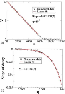
where M denotes the number of different initial conditions 共particles兲in the ensemble. In this paper, all simulations were performed usingM= 104. As we see in Fig.2共a兲, the average velocity decays linearly as a function of the number of col-lisions with the boundary. The slope of the decay was obtained via a linear fit as −0.001530共2兲 where the term 2 ⫻10−6represents the error of the fitting. Eventually, the par-ticle reaches a critical velocity after leaving the collision zone and has no energy to reach the boundary again for the next collision and, after having all of its energy dissipated by the drag force, it stops. The plateau seen in Fig. 2共a兲for n ⬎7000 represents few orbits which stay with low velocity after the linear decay is finished before stopping completely. We have simulated the behavior of the decay of the par-ticle’s velocity for many different control parameters. The slope of the decay as a function of the control parameteris shown in Fig. 2共b兲. It was shown analytically关32兴, that the behavior of the decay of the particle’s velocity for the Fermi-Ulam model共a classical particle bouncing between two rigid walls, where one of them is fixed and the other one moves periodically in time兲is linearly dependent on the control pa-rameter, i.e.,Vn⬀V0− 2n. It is worth mentioning that the Fermi-Ulam model is a one-dimensional共1D兲system. In our case however, the dynamics might be considered as a gener-alization of the Fermi-Ulam model to two-dimensional共2D兲 and therefore, as shown in Fig. 2共b兲, the behavior of the average velocity of the particle isVn⬀V0− 1.5314共3兲n. The results obtained allow to conclude that if the particle experi-ences a drag force proportional to its velocity, the phenom-enon of unlimited energy growth共FA兲is suppressed.
B. Results for the caseF= −V2
The equation that needs to be integrated is −V2=dV/dt.
Considering the initial velocity asVn⬎0, we obtain that
V共t兲= Vn
1 +共t−tn兲, 共12兲
with tⱖtn. The integration of Eq. 共12兲 gives the displace-ment of the particle
FIG. 2. 共Color online兲 共a兲 Behavior of the average velocity as function of n. The control parameters used were⑀= 0.1,a= 0.1,p = 3, and= 10−3and the initial velocity wasV
r共t兲= 1
ln关1 +Vn共t−tn兲兴, 共13兲
fortⱖtn. Updating the mapping with Eqs.共12兲and共13兲, we can then follow the dynamics of the particle. The behavior of V
¯ as function of n is shown in Fig.3共a兲. For a large initial velocity, sayV0= 10, the velocity of the particle experiences an exponential decay for a short time and then, after reaching a characteristic crossover, saync, the velocity bends toward a regime of a constant plateau. Contrary to the case of F⬀−V, the dissipation does not stop the dynamics of the particle sincer共t兲is a function which grows in time. There-fore, the particle keeps moving and the dissipation gets smaller as the velocity of the particle diminish. Furthermore, if the particle has escaped the collision zone, it enters it again and suffers another collision with the boundary. An exponen-tial fitting for the decay shown in Fig. 3共a兲 gives that V¯ =V0exp关−0.00153共1兲n兴 for the control parameter = 10−3. We performed the simulations for many different control pa-rameters and obtained the slope of the decay for each one of them. Figure 3共b兲 shows the behavior of the slope of the decay as a function of the control parameter . A linear fit-ting gives the slope ⬀−1.482共4兲. A comparison with the Fermi-Ulam model can also be made. As discussed in 关33兴, the decay of the velocity in the Fermi-Ulam model was ob-tained analytically as Vn=V0exp关−2n兴. However, in the time-dependent oval billiard, we have found that Vn =V0exp关−1.482共4兲n兴. Therefore, the decay obtained for the oval billiard is slower for both cases 共i兲and共ii兲what is probably associated with the dimensionality of the system. This difference might also be caused by the fact that there is now a competition between production and suppression of FA, while Fermi-Ulam model does not exhibit FA at all.
Consider now the behavior of the average velocity for large values of n, i.e., along the constant plateau. The zoom in Fig.3共a兲shows few points along the constant plateau. We see that it fluctuates around an average value and does not decreases to zero. But the question is: how changes the av-erage velocity along the plateau if the strength of the dissi-pation is changed? If a reduction takes place, it is expected that dissipation affects the FA less and, therefore, the con-stant plateau should rise. It does indeed happens. The behav-ior ofVplateauas function ofis shown in Fig.4共a兲. A power law fitting gives us that Vplateau⬀−0.5. Thus, as the control parameter→0, the velocity diverges, recovering FA. This behavior characterizes a smooth transition from suppression to production of FA. Figure4共b兲 shows the behavior of the crossover iteration numbernc, which is the number of colli-sions with the boundary needed to change the regime of decay to the regime of constant velocity, for the initial ve-locityV0= 10. The ensemble used was a grid of 100⫻100 for the variables ␣0苸关0 ,兴⫻0苸关0 , 2兴. A power law fitting applied to Fig. 4共b兲yieldsnc⬀−0.869共2兲.
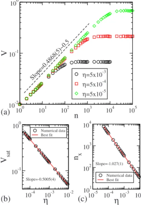
We now discuss the behavior of the average velocity of the particle when a given initial velocity is very small compared to the maximum component of the moving boundary velocity. The behavior of the average velocity as function of n is shown in Fig. 5共a兲. One can clearly see that the average velocity starts growing for smallnand then, after reaching a critical crossover nx, it bends toward a re-gime of saturation, marked by a constant plateau. As the damping coefficient decreases, the average velocity can reach higher values. Moreover the crossover also rises. We then suppose that
共i兲 For smalln, say nⰆnx, the average velocity is given by
FIG. 3. 共Color online兲 共a兲The average velocity as function ofn for an initial V0= 10. The control parameters used were ⑀= 0.1,a = 0.1,p= 3, and= 10−3.共b兲Linear fit of the slope of the velocity’s decay as a function of.
10-4 10-3 10-2
η 10-1
100
Vplateau
Numerical data Power law fit
10-4 10-3 10-2
η 103
104
n c
Numerical data Power law fit Slope=-0.5005(4)
Slope=-0.869(2) (a)
(b)
V
¯⬀n, 共14兲
whereis a critical exponent;
共ii兲For very large n, i.e.,nⰇnx, the average velocity is written as
V ¯
sat⬀␥, 共15兲
and␥is also a critical exponent;
共iii兲 Finally, the crossover nx, which marks the change from the regime of growth to the saturation is given by
nx⬀z
, 共16兲
wherezis a critical exponent.
Using the formalism shown in 关37,38兴, it is possible to describe the behavior ofV¯ using a scaling function. The criti-cal exponents are obtained by numericriti-cal fittings as shown in Figs. 5共b兲 and 5共c兲, and the obtained values were  = 0.4868共5兲 ⬵0.5, ␥= −0.5005共4兲 ⬵−0.5, and z= −1.027共1兲 ⬵−1. Using these three values, we can rescale the axis and obtain a single and universal plot, as shown in Fig.6.
We now discuss the critical exponents and the transition. First, it is important to mention that, as the damping coeffi-cient →0, the unlimited energy growth is recovered, as described by Eq.共15兲given that␥= −0.5. Since FA is recov-ered, the crossover nx also diverges for →0, as easily checked from Eq. 共16兲 for z= −1. The critical exponents obtained for the phase transition from limited to unlimited
energy growth in this section are the same as those obtained from the dissipative bouncer model关37,38兴 共a classical par-ticle suffering inelastic collisions with a periodically moving wall in the presence of a constant gravitational field兲. Despite the two models are very different, e.g., the bouncer model is a 1D system and the particle experiences the action of a constant gravitational field, while the driven oval-like shaped billiard is a 2D system, the dissipation used in the bouncer model is qualitatively different from the dissipation used in this section, the phase transition from limited to unlimited energy exhibits the same critical exponents. Therefore the two models belong to the same class of universality near this phase transition. In principle the classification of univer-sality classes is made only using the critical exponents␥,, andz.
If one think a little bit deeper in the dynamics, when the restitution coefficient in the bouncer model approaches the unity, the dissipative dynamics is replaced by nondissi-pative one and chaotic attractors no longer exist anymore. The interval of time between impacts is then proportional to the particle’s velocity 共⌬t⬀V兲. With increasing velocity the time between collisions increases too leading to a loss of correlation between the impacts. This leads to an in-crease of randomness in the system therefore producing unlimited energy growth. In the oval-like billiard, when the damping coefficient approaches zero 共no dissipation兲, as opposite to the bouncer model, the time between im-pacts is inversely proportional to the particle’s velocity 共⌬t⬀V−1兲. For fixed boundary there exist a smooth transi-tion from dissipative to conservative dynamics 关28兴, thus, leading the phase space in the angular coordinates to show mixed form 关28,29兴. Such a mixed structure however pro-duces conservative chaotic portions in the phase space that is what the LRA conjecture claims 关24兴 as needed to observe FA when time perturbation to the boundary is intro-duced. Basically chaotic dynamics works more like stochas-tic behavior yielding in diffusion in the average velocity and hence leading the particle to experience FA. Despite the dif-ferences between the two models and the different mecha-nisms which produce FA, the behavior of the average veloc-ity near a transition from dissipative to no dissipative dynamics is described by the same law with the same critical exponents.
100 101 102 103 104 105
n
10-2 10-1 100
V
η=5x10⁻³ η=5x10⁻⁴ η=5x10⁻⁵
10-4 10-3 10-2
η
10-1 100
Vsat
Numerical data Best fit
10-5 10-4 10-3 10-2
η
101 102 103 104
n x
Numerical data Best fit Slope=0.4868(5)~0.5
Slope=-0.5005(4)
Slope=-1.027(1)
(a)
(b) (c)
FIG. 5. 共Color online兲 共a兲The average velocity as function ofn for three different control parameters, as labeled in the figure. The initial velocity used wasV0= 10−2and the control parameters were ⑀= 0.1, a= 0.1 and p= 3. 共b兲 Plot of V¯sat versus . A power law fitting yields the slope␣= −0.5005共4兲.共c兲Plot ofnxversus. The slope obtained isz= −1.027共1兲.
C. Results for the caseF= −V␦
In this section, we consider the dissipationF= −V␦with 1⬍␦⬍2, acting in the particle. Taking the initial velocity as Vn⬎0 and integrating the equation of motion we obtain
V共t兲=关Vn1−␦−共1 −␦兲共t−tn兲兴1/1−␦
, 共17兲
with tⱖtn and ␦⫽1. The displacement of the particle is therefore obtained by the integration of dr/dt=V共t兲, which gives
r共t兲= Vn 2−␦
共2 −␦兲−
关Vn1−␦−共1 −␦兲共t−tn兲兴2−␦/1−␦
共2 −␦兲 , 共18兲
with␦⫽1,␦⫽2 andtⱖtn. Depending on the control param-eter␦, the dissipation can lead to a complete stopping of the particle. We illustrate the typical regimes of the displacement of the particle in Figs.7共a兲and7共b兲by some plots ofr⫻tfor = 10−2 and for two different values ofV0, namely: 共a兲 V0 = 10−3and共b兲V0= 10−2. The control parameter␦is labeled in the figure. Since in the process of motion the particle may acquires small values of the velocity, then depending on the coordinate angle of the particle’s trajectory, all of its energy may dissipate, thus stopping the dynamics. Such a behavior is not observed for values of␦⬎1.48.
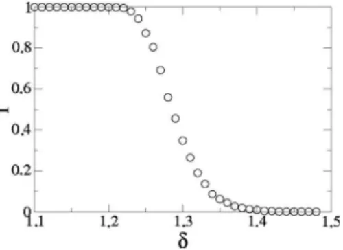
We also evaluated the fraction of initial conditions, f, which reaches the rest as function of the control parameter␦. This fraction is obtained by evolving a grid of 100⫻100 different initial conditions␣0苸关0 ,兴and0苸关0 , 2兴for an initial velocity V0= 1 and random t0苸关0 , 2兴 for a fixed damping coefficient= 10−3and the fixed control parameters p= 3,⑀= 0.1 anda= 0.1. When the particle stops, then a new initial condition is taken. Since the simulations are very com-putational time consuming, we impose some criteria to stop evolving the orbit. If the particle did not stop after 105 col-lisions with the boundary, a new initial condition is started and the previous orbit is not used to compute f. A plot of f versus ␦ is shown in Fig. 8. If ␦⬍1.2, then the particles always stop. Moreover, for 1.2⬍␦⬍1.48, there is a mono-tonic decay of f and for␦⬎1.48, no initial conditions have their total energy dissipated up to 105 collisions with the boundary.
The limits of the relations Eqs.共17兲 and共18兲for both ␦ →1 and ␦→2 can be obtained. Expanding Eq. 共17兲 for ␦ →1 and taking only the first order, we have that
V共t兲=Vnexp关−共t−tn兲兴+ 䊊共␦− 1兲, 共19兲 while the same procedure for Eq.共18兲gives that
r共t兲=Vn 关1 −e
−共t−tn兲兴
+ 䊊共␦− 1兲. 共20兲
We see that both Eqs.共19兲and共20兲recover the case of linear damping force and therefore lead to linear decay of the ve-locity, as demonstrated before.
On the other hand, for␦→2, the expansions of Eqs.共17兲 and共18兲give that
V共t兲= Vn
1 +共t−tn兲+ 䊊共␦− 2兲, 共21兲
r共t兲= 1
ln关1 +Vn共t−tn兲兴+ 䊊共␦− 2兲, 共22兲
which lead therefore to an exponential decay in the velocity of the particle for␦→2, as shown before. For different val-ues of␦, say 1⬍␦⬍2, the decay of the velocity is generally FIG. 7. 共Color online兲 共a兲Plot ofrversustfor different values
of the exponent␦, as shown in the figure. The initial velocity used wasV0= 10−3.共b兲Same plot of共a兲for initial velocityV0= 10−2.
a power-like, as one can see in Fig.9for␦= 1.5. The damp-ing coefficient used was = 10−3 and the best fitting, given by a second order polynomial in n is V共n兲= 10.02共1兲 − 0.00485共1兲n+ 5.871共1兲⫻10−7n2.
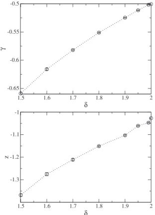
Let us now extend the procedure used in Sec. III B to describe the behavior of the average velocity and hence the critical exponents that describe the transition from limited to unlimited energy growth. According to Fig.8, termination of the dynamics is observed for ␦⬍1.48. Since we want characterize the phase transition from limited to unlimited energy growth, the range considered is␦ⱖ1.5 and termina-tion of the dynamics is avoided. A plot of the average veloc-ity against n for ␦= 1.99 is shown in Fig. 10. We see that average velocity behaves quite similar to the case described in Sec. III B and that the scaling hypotheses also are the same as those described by Eqs. 共14兲–共16兲. However, the critical exponents obtained are rather different and depend on ␦. We have considered seven different values of ␦ and ob-tained the critical exponents ␥ and z, as shown in Table I. Extensive numerical simulations were carried out moreover leading to an average¯= 0.480共3兲 ⬵0.5. To confirm the va-lidity of the scaling hypotheses, universal plots were ob-tained, as shown in Fig.11 for different values of ␦ and at least three different values of. A plot of the critical expo-nents as function of the control parameter␦ is shown in Fig.
12. We see that as the control parameter␦rises, both critical
exponents exhibit a monotonically growth. As ␦→2, the critical exponent␥→−0.5 andz→−1. The exponents shown in TableI, thus, confirm that FA will take place in the limit of vanishingly dissipation and that such a transition is smooth.
IV. CONCLUDING REMARKS
We have studied some dynamical properties of billiards in a driven oval-like shaped domain under three different types of a drag force. For a damping force proportional to the particle’s velocity, we have shown that the particle experi-ences a linear decay on the velocity and that the speed of the FIG. 9. 共Color online兲Decay of the velocity of the particle for
␦= 1.5. The control parameters used were p= 3,⑀= 0.1, anda= 0.1 and the damping coefficient= 10−3. The best fitting, by the second degree polynomial is V共n兲= 10.02共1兲− 0.00485共1兲n+ 5.871共1兲 ⫻10−7n2.
FIG. 10. 共Color online兲Plot ofV¯ versusnfor␦= 1.99 and dif-ferent values of, as labeled in the figure.
TABLE I. Critical exponents␥andzobtained for different val-ues of␦, as labeled in the Table.
␦ ␥ z
1.5 −0.659共2兲 −1.368共6兲
1.6 −0.616共2兲 −1.275共7兲
1.7 −0.582共1兲 −1.211共5兲
1.8 −0.5511共9兲 −1.151共3兲
1.9 −0.5246共6兲 −1.103共3兲
1.95 −0.5115共6兲 −1.061共2兲
1.99 −0.5017共5兲 −1.047共2兲
2.0 −0.5005共4兲 −1.027共1兲
10-4 10-2 100 n/ηz
10-4 10-3
V/
η
γ
η=10-4
η=5X10⁻⁴
η=10-3
10-4 10-2 100 102 n/ηz
10-4 10-3
V/
η
γ
10-4 10-2 100 102 n/ηz
10-4 10-3
V/
η
γ
10-4 10-2 100 102 n/ηz
10-4 10-3
V/
η
γ
(a) (b)
(c) (d)
δ=1.6 δ=1.8
δ=1.9 δ=1.99
decay is proportional to −1.5, thus far slow as compared to the Fermi-Ulam model 关32兴. Our results therefore confirm that FA is suppressed and the particle stops. For the case of a drag force proportional to a square of the velocity of the
particle, our results confirm that FA also is suppressed. The decay of the particle’s velocity is of an exponential type with the exponent of the order of −1.5, therefore also slower than in the Fermi-Ulam model 关33兴. As the velocity of the particle decreases, the damping force decays faster and the particle never stops. We have shown that, starting with a small energy, the velocity of the particle could be described with the help of scaling. As the damping coefficient →0, the particle experiences a phase transition from limited to unlimited energy growth. The critical expo-nents obtained are the same as those for the dissipative bouncer model 关37,38兴. Despite the differences of the two models, the criticality near such a phase transition is the same. Therefore, near this phase transition, the two models belong to the same class of universality. As the control pa-rameter␦varies, the particle can stops. The fraction of initial conditions for which it happens was computed as function of ␦ for an ensemble of 104 initial conditions. For ␦⬍1.2, all the initial conditions lead the dynamics to stop. However, for 1.2⬍␦⬍1.48, there is a monotonic decay of f while for ␦ ⬎1.48, none of the initial conditions have their total energy dissipated in the process of numerical simulations, i.e., up to 105 collisions with the boundary. Critical exponents charac-terizing a phase transition from limited to unlimited energy growth were also obtained from different values of ␦, as shown in Table I.
ACKNOWLEDGMENTS
The work of E.D.L. was partially supported by CNPq, FAPESP, and FUNDUNESP, Brazilian agencies. He also ac-knowledges support for a visit to Georgia Tech from comis-são mista CAPES/FULBRIGHT. L.B. was partially sup-ported by NSF共Grant No. DMS-0900945兲.
关1兴N. Chernov and R. Markarian, Chaotic Billiards 共American Mathematical Society, Providence, 2006兲, Vol. 127.
关2兴M. V. Berry,Eur. J. Phys. 2, 91共1981兲.
关3兴L. A. Bunimovich,Commun. Math. Phys. 65, 295共1979兲.
关4兴D. Sweetet al.,Physica D 154, 207共2001兲.
关5兴H. D. Graf, H. L. Harney, H. Lengeler, C. H. Lewenkopf, C. Rangacharyulu, A. Richter, P. Schardt, and H. A. Weiden-muller,Phys. Rev. Lett. 69, 1296共1992兲.
关6兴T. Sakamotoet al.,Jpn. J. Appl. Phys. 30, L1186共1991兲.
关7兴J. P. Bird,J. Phys.: Condens. Matter 11, R413共1999兲.
关8兴E. Persson, I. Rotter, H. J. Stockmann, and M. Barth, Phys. Rev. Lett. 85, 2478共2000兲.
关9兴E. D. Leonel,Phys. Rev. Lett. 98, 114102共2007兲.
关10兴J. Stein and H. J. Stockmann, Phys. Rev. Lett. 68, 2867 共1992兲.
关11兴H. J. Stökmann,Quantum Chaos: An Introduction共Cambridge University Press, Cambridge, England, 1999兲.
关12兴V. Milner, J. L. Hanssen, W. C. Campbell, and M. G. Raizen,
Phys. Rev. Lett. 86, 1514共2001兲.
关13兴N. Friedman, A. Kaplan, D. Carasso, and N. Davidson,Phys. Rev. Lett. 86, 1518共2001兲.
关14兴M. F. Andersen, T. Grunzweig, A. Kaplan, and N. Davidson,
Phys. Rev. A 69, 063413共2004兲.
关15兴M. F. Andersen, A. Kaplan, T. Grunzweig, and N. Davidson,
Phys. Rev. Lett. 97, 104102共2006兲.
关16兴C. M. Marcus, A. J. Rimberg, R. M. Westervelt, P. F. Hopkins, and A. C. Gossard,Phys. Rev. Lett. 69, 506共1992兲.
关17兴E. Fermi,Phys. Rev. 75, 1169共1949兲.
关18兴A. Y. Loskutov, A. B. Ryabov, and L. G. Akinshin, J. Exp. Theor. Phys. 89, 966共1999兲.
关19兴P. J. Holmes,J. Sound Vib. 84, 173共1982兲.
关20兴A. K. Karlis, P. K. Papachristou, F. K. Diakonos, V. Constan-toudis, and P. Schmelcher,Phys. Rev. Lett. 97, 194102共2006兲;
Phys. Rev. E 76, 016214共2007兲.
关21兴A. J. Lichtenberg and M. A. Lieberman,Regular and Chaotic Dynamics, Applied Mathematical Sciences 共Springer-Verlag, New York, 1992兲, Vol. 38.
关22兴D. G. Ladeira and Jafferson Kamphorst Leal da Silva, Phys. Rev. E 73, 026201共2006兲.
关23兴A. Loskutov and E. D. Leonel, Math. Probl. Eng. 共2009兲, 848619.
关24兴A. Loskutov, A. B. Ryabov, and L. G. Akinshin,J. Phys. A 33, 7973共2000兲.
关25兴F. Lenz, F. K. Diakonos, and P. Schmelcher,Phys. Rev. Lett.
1.5 1.6 1.7 1.8 1.9 2
δ
-0.65 -0.6 -0.55 -0.5
γ
1.5 1.6 1.7 1.8 1.9 2
δ
-1.3 -1.2 -1.1 -1
z
100, 014103共2008兲.
关26兴D. F. M. Oliveira and E. D. Leonel, Physica A 389, 1009 共2010兲.
关27兴E. D. Leonel and L. A. Bunimovich, Phys. Rev. Lett. 104, 224101共2010兲.
关28兴A. Arroyo, R. Markarian, and D. P. Sanders,Nonlinearity 22, 1499共2009兲.
关29兴D. F. M. Oliveira and E. D. Leonel,Commun. Nonlinear Sci. Numer. Simul. 15, 1092共2010兲.
关30兴S. O. Kamphorst, E. D. Leonel, and J. K. L. da Silva,J. Phys. A: Math. Theor. 40, F887共2007兲.
关31兴E. D. Leonel, D. F. M. Oliveira, and A. Loskutov,Chaos 19, 033142共2009兲.
关32兴E. D. Leonel and P. V. E. McClintock, Phys. Rev. E 73,
066223共2006兲;J. Phys. A 39, 11399共2006兲.
关33兴E. D. Leonel and D. F. Tavares,CP913, Nonequilibrium Sta-tistical Mechanics and Nonlinear Physics, XV Conference, ed-ited by O. Descalzi, O. A. Rosso, and H. A. Larrondo,共 Ameri-can Institute of Physics, New York, 2007兲, Vol. 108.
关34兴M. Robnik and M. V. Berry,J. Phys. A 18, 1361共1985兲.
关35兴M. V. Berry and E. C. Sinclair,J. Phys. A 30, 2853共1997兲.
关36兴M. Aichinger, S. Janecek, and E. Rasanen,Phys. Rev. E 81, 016703共2010兲.
关37兴E. D. Leonel and A. L. P. Livorati, Physica A 387, 1155 共2008兲.
关38兴Andre Luis Prando Livorati, D. G. Ladeira, and E. D. Leonel,