www.nat-hazards-earth-syst-sci.net/14/259/2014/ doi:10.5194/nhess-14-259-2014
© Author(s) 2014. CC Attribution 3.0 License.
Natural Hazards
and Earth System
Sciences
Sample size matters: investigating the effect of sample size
on a logistic regression susceptibility model for debris flows
T. Heckmann1, K. Gegg1, A. Gegg2, and M. Becht1
1Physical Geography, Catholic University of Eichstaett-Ingolstadt, Ostenstr. 18, 85072 Eichstaett, Germany 2Statistics, Catholic University of Eichstaett-Ingolstadt, Ostenstr. 26, 85072 Eichstaett, Germany
Correspondence to:T. Heckmann ([email protected])
Received: 21 May 2013 – Published in Nat. Hazards Earth Syst. Sci. Discuss.: 21 June 2013 Revised: 5 December 2013 – Accepted: 9 January 2014 – Published: 17 February 2014
Abstract.Predictive spatial modelling is an important task in natural hazard assessment and regionalisation of geomorphic processes or landforms. Logistic regression is a multivariate statistical approach frequently used in predictive modelling; it can be conducted stepwise in order to select from a num-ber of candidate independent variables those that lead to the best model. In our case study on a debris flow susceptibil-ity model, we investigate the sensitivsusceptibil-ity of model selection and quality to different sample sizes in light of the following problem: on the one hand, a sample has to be large enough to cover the variability of geofactors within the study area, and to yield stable and reproducible results; on the other hand, the sample must not be too large, because a large sample is likely to violate the assumption of independent observations due to spatial autocorrelation. Using stepwise model selection with 1000 random samples for a number of sample sizes between n= 50 andn= 5000, we investigate the inclusion and exclu-sion of geofactors and the diversity of the resulting models as a function of sample size; the multiplicity of different mod-els is assessed using numerical indices borrowed from in-formation theory and biodiversity research. Model diversity decreases with increasing sample size and reaches either a local minimum or a plateau; even larger sample sizes do not further reduce it, and they approach the upper limit of sample size given, in this study, by the autocorrelation range of the spatial data sets. In this way, an optimised sample size can be derived from an exploratory analysis. Model uncertainty due to sampling and model selection, and its predictive ability, are explored statistically and spatially through the example of 100 models estimated in one study area and validated in a neighbouring area: depending on the study area and on sam-ple size, the predicted probabilities for debris flow release
differed, on average, by 7 to 23 percentage points. In view of these results, we argue that researchers applying model se-lection should explore the behaviour of the model sese-lection for different sample sizes, and that consensus models created from a number of random samples should be given prefer-ence over models relying on a single sample.
1 Introduction
can occur and/or have occurred in the larger area wherever the conditions are equal or similar to those in the surveyed area and (ii) that future events will take place under condi-tions the same as or similar to those in the past (e.g. Fabbri et al., 2003).
In this study, we apply the method of multivariate logis-tic regression to the identification of potential debris flow initiation sites in a high mountain catchment; the spatial unit is the raster cell (as opposed to e.g. slope units; see Van Den Eeckhaut et al., 2009). Together with discriminant analysis (e.g. Baeza and Corominas, 2001), soft comput-ing techniques – such as “weights of evidence” (Bonham-Carter, 1994; Neuhäuser and Terhorst, 2006) or “certainty factor” (e.g. Binaghi et al., 1998) – and artificial neural networks (e.g. Lee et al., 2003; Ermini et al., 2005; Liu et al., 2006), logistic regression belongs to the most fre-quently chosen approaches to spatial modelling of land-slides (Atkinson et al., 1998; Ohlmacher and Davis, 2003; Beguería and Lorente, 2003; Brenning, 2005; Ayalew and Yamagishi, 2005; Beguería, 2006; Van Den Eeckhaut et al., 2006; Meusburger and Alewell, 2009; Van Den Eeckhaut et al., 2010; Atkinson and Massari, 2011; Ruette et al., 2011; Guns and Vanacker, 2012). Recently, some published studies dealt specifically with debris flow susceptibility models on the regional scale; for the identification of potential release areas, a range of different approaches has been used, includ-ing heuristic (Horton et al., 2008; Kappes et al., 2011; Fischer et al., 2012) and statistical ones (Heckmann and Becht, 2009; Blahut et al., 2010a, b). The so-delineated release areas can be used as starting points for models that predict the path-ways, lateral extent, runout length and other relevant proper-ties of debris flows (e.g. Blahut et al., 2010b; Kappes et al., 2011), which is important for hazard assessment and has also been used in geomorphological applications, for exam-ple research on sediment cascades (Wichmann et al., 2009; Heckmann and Schwanghart, 2013).
In order to use a model for prediction, a sample has to be drawn, and the model parameters of the population are esti-mated based on that sample. Sampling is essential, because event and non-event units show spatial autocorrelation (see Sect. 1.2), and dependent data lead too easily to the rejection of null hypotheses and the incorrect declaration of parame-ters as significant; Legendre (1993) explains this for ecolog-ical models (see also Van Den Eeckhaut et al., 2006). Using a stepwise approach, the predictor variables for an effective yet parsimonious model are selected from a set of candidate geofactors (Sect. 3.2.2). Brenning (2005) found that logistic regression with stepwise variable selection yielded the low-est error rates in his comparison of different statistical meth-ods. Logistic regression was also the best single method in the comparative study by Rossi et al. (2010), and exhibited the highest area under the curve (AUC) for “fine slope units” (second rank in overall comparison) in Carrara et al. (2008), a study specifically referring to debris flows.
The choice of predictor variables will understandably de-pend on the sample (Guns and Vanacker, 2012), and it is also clear that the aim of every susceptibility model should be a reliable and reproducible prediction. This prediction should not depend too much on the sample that is taken in order to select the variables and estimate the model param-eters. Several previous studies do not involve sampling at all (e.g. Ohlmacher and Davis, 2003; Ruette et al., 2011); i.e. they use all available data for estimating the model pa-rameters. The majority of studies use only one single sample (e.g. Atkinson et al., 1998; Van Den Eeckhaut et al., 2006; Meusburger and Alewell, 2009), the size of which usually depends on the number or size of landslide initiation zones (see Sect. 1.1). Recognising the dependence of model results on the sample, Brenning (2005) takes 50 samples to com-pare error rates across different sample sizes and statistical methods. Beguería (2006) and Guns and Vanacker (2012) ap-ply 50-fold replication in order to estimate the robustness of the modelling result with respect to sampling, and Van Den Eeckhaut et al. (2010) calculate an ensemble of 25 mod-els from different samples of their data. Hjort and Marmion (2008) conduct repeat sampling to explore the influence of sample size on the predictive power of (among others) multi-ple logistic regression models for predictive geomorphologi-cal mapping.
The present study has two main foci that will be devel-oped in detail in the following subsections. It is not the aim of our study to find out the best performing method for a debris flow susceptibility model (comparative studies of pre-dictive models were carried out, for example, by Brenning, 2005; Marmion et al., 2008; Carrara et al., 2008; Vorpahl et al., 2012); we deliberately chose logistic regression for its widespread use, and for the relevant assumption of sam-ple independence which we found to be frequently neglected in previous studies. First, we explore the sensitivity of step-wise model selection to sample size. Sections 1.1 and 1.2 will explain why the sample size must neither be too small nor too large. In this context, the main aim of the study is to investigate if an “optimal” sampling size can be found as a compromise between samples too small and too large. Second, we quantify the uncertainty inherent in a stepwise modelling approach, with respect to (i) the selection of ge-ofactors, (ii) model parameters, and (iii) the spatial pattern of uncertainty in the resulting susceptibility map. This study aim will be developed in Sect. 1.3.
1.1 Constraints on sample size 1: why the sample must not be too small
cause the estimation to be uncertain, and there is a higher risk of coefficients being insignificant when the respective confidence interval includes zero. With respect to replicate sampling and model selection, it is expected that the diver-sity of models (and hence the dependence of the models on the sample) will be large in this case.
Moreover, in a large study area, a small sample is unlikely to cover the variability of geofactors, especially if several of them are part of the model. Here, a larger sample would in-clude more information on the study area and would possibly provide a better model. There are rules of thumb that estimate the minimum sample size for a regression analysis on the ba-sis of a constant (e.g.>50), of the ratio of observations and predictor variables, or of a combination of the latter; such rules have been explored in light of significance, power and effect size, e.g. by Green (1991), who found “some support” for the rule of thumbnmin≥50+8m, wherenminis the min-imum sample size andmis the number of predictor variables. In this study, when we speak of sample size, we always address a sample of “non-events”, i.e. a sample of raster cells without debris flow initiation. If a random sample referred to all raster cells, including event and non-event cells, the num-ber of event cells in the sample would certainly be smaller than in the original inventory. This would cause a loss of in-formation particularly for those cells that represent the target of the modelling exercise; therefore, all initiation areas will be represented in the models and only the size of the event sample is varied in our investigation. Besides the non-event sample size, the relative sample sizenrel(i.e. the areal extent of the total sample divided by the size of the study area) will be reported.
1.2 Constraints on sample size 2: why the sample must not be too large
While it is intuitive that larger samples contain more infor-mation that can be used by the model, and the model might be better, there are several reasons why the sample size must not be too large either.
King and Zeng (2001) argue that the non-event sample size has to be kept as small as possible because of the dispro-portionate cost and effort of acquiring data for many vari-ables and observations that are not related to the target phe-nomenon (event). Like in political science, the acquisition of observations is costly in ecology (with the application of regression models to the spatial prediction of species distri-bution). In this context, the complexity of the investigated systems is reflected in large numbers of predictors; more-over, the logistic difficulty of mapping the presence or ab-sence of a species in large and remote areas should not be underestimated (see e.g. Stockwell and Townsend Peterson, 2002). An important justification for predictive geomorpho-logical mapping (Luoto and Hjort, 2005) is that area-wide field mapping is time-consuming, difficult in remote or inac-cessible areas, and may suffer from subjectivity (van Asselen
and Seijmonsbergen, 2006; Hjort and Marmion, 2008). How-ever, in contrast to the examples from political and ecolog-ical science, many if not most variables in predictive geo-morphological mapping are easily derived from digital ele-vation models and remote sensing data; both are available globally, with ever-increasing accuracy and resolution. This does not change the effort required for mapping the target phenomenon (“events”), but the motivation for limiting sam-ple size of non-events appears to be quite different, as it does not so much refer to the effort of data acquisition (quantity and quality). In order to limit the sample size and to mitigate the rare-events issue (see below), the literature suggests dif-ferent ratios of event : non-event sample sizes, mostly with-out justifying the particular choice of this ratio. Instead of merely adopting one of these suggestions (which generally range from 1 : 1 to 1 : 10), our paper aims at an empirical analysis of sample dependence and performance of the sus-ceptibility model as a function of sample size.
Other reasons for restricting sample size are overparame-terisation and overfitting of the model (Hjort and Marmion, 2008, and references therein). Increasing sample sizes causes standard errors and confidence intervals in parameter esti-mation to decrease. In a significance-based stepwise model selection, very large samples are expected to facilitate the inclusion of more and more variables (risk of overparam-eterisation). Such inclusion of more information does not necessarily lead to better model performance; Stockwell and Townsend Peterson (2002) describes “plateaus” wherein new data add little to model performance. In some cases, inclu-sion of more data even causes worse performance, because a model fit to a very specific set of information may perform poorly on new data (risk of overfitting; see Stockwell and Townsend Peterson, 2002, and references therein). Brenning (2005), however, states that overfitting is “not a serious prob-lem for logistic regression”, contrary to machine-learning methods (cf. Petschko et al., 2014, and references therein).
be uncorrelated), and that this may lead to “incoherent sig-nificance estimates for the parameters” (see also Brenning, 2005). Consequently, such incoherent estimates compromise both significance-based model selection and the assessment of parameter importance that is based on the latter.
In previous studies applying logistic regression to land-slide susceptibility analysis, the problem of stochastically dependent samples has frequently been ignored (e.g. by us-ing all available data instead of a sample; see above). In some instances, the risk of autocorrelation is dealt with for events only, as geofactors tend to be homogeneous (and consequently strongly autocorrelated) on landslide terrain (Atkinson and Massari, 2011). However, the independence assumption refers to all observations of the dependent vari-able (Hosmer and Lemeshow, 2000; Van Den Eeckhaut et al., 2006), in our case to the occurrence and non-occurrence of debris flow initiation. As the geofactors used as independent variables are supposed to be associated with the dependent variable, we argue that the degree of autocorrelation of these geofactors should be accounted for in the sampling proce-dure. In order to mitigate the issue of spatial autocorrela-tion, some authors choose one raster cell for each landslide source area on a systematic basis. Atkinson et al. (1998) and Van Den Eeckhaut et al. (2006), for example, use the cen-tre of each landslide source area. Similarly, Vanwalleghem et al. (2008) use the centre of each topographic depression, and the centre of each gully in their study predicting the spatial distribution of closed depressions and gullies under forest. Different authors draw samples of source areas on different grounds; besides spatial autocorrelation, Atkinson et al. (1998) explain their approach with the aim of prevent-ing model bias towards larger landslides – in a full sample of events, more data would enter the model from larger source areas than from smaller ones. Beguería and Lorente (2003) use one raster cell for each debris flow initiation zone be-cause the raster size (10 m) of the data in their study cor-responds to the size of a typical debris flow scar. All ap-proaches have in common that they prevent a contiguous (and hence potentially strongly spatially autocorrelated) sample of hundreds of landslide initiation cells from entering the model. Spatial autocorrelation has also been accounted for in model validation (Brenning, 2005). However, as Atkinson and Massari (2011) point out, autocorrelation in the geofac-tors is frequently not adequately accounted for in the regres-sion model. While the latter study proposes an autologistic model (see also Brenning, 2005), we will try to warrant inde-pendence of observations through the choice of an adequate sampling size (see Sect. 3.3.2): as the number of sampled raster cells in a finite study area increases, the average dis-tance between those cells will decrease, and finally the in-dependence assumption will no longer hold given the spatial autocorrelation of the geofactors.
Normally, a logistic regression model is fit to a sam-ple where the ratio of event : non-event cases is approxi-mately 1 : 1. Then, the so-called cutoff, i.e. the value of
the model result that discriminates between event and non-event, equals 0.5. King and Zeng (2001) explain that the number of non-events should be typically 2–5 times higher than that of events. In this case, the cutoff needed to trans-late the model result to a classification (event or non-event) would need to be adjusted accordingly. Because the ratio of event : non-event spatial units (not only raster cells but also lumped spatial units; Beguería and Lorente, 2003) usu-ally is by far smaller, a bias towards small probabilities arises.1 This problem has been addressed by the develop-ment of “rare events logistic regression” (King and Zeng, 2001). Besides endogenous stratified sampling (a sampling strategy that includes all events plus a random sample of non-events), these authors propose corrections for the inter-cept and for the estimated probabilities. Rare-events logistic regression was applied in landslide susceptibility modelling by Van Den Eeckhaut et al. (2006) and Guns and Vanacker (2012). In many studies, endogenous stratified sampling has been adopted, and the authors chose event : non-event ratios of 1 : 1 (e.g. Brenning, 2005; Meusburger and Alewell, 2009; Van Den Eeckhaut et al., 2010), 1 : 2 (Wang and Sassa, 2005), 1 : 5 (Van Den Eeckhaut et al., 2006), or 1 : 10 (Beguería and Lorente, 2003; Beguería, 2006; Guns and Vanacker, 2012). Finally, Atkinson et al. (1998), who use only the central cell of each landslide as the event sample, sample as many non-event cells as required in order to attain the ratio of landslide to non-landslide area.
In our study, we adopt stratified random sampling by a ran-dom sample of one cell for each debris flow initiation zone, and a random sample of non-event cells. The size of the latter is then varied in order to explore the effect on stepwise model selection; hence, we do not pre-select an event : non-event ra-tio. Rare-event correction according to King and Zeng (2001) is not applied.
1.3 Uncertainty: model selection, parameters, spatial patterns
The result of the investigations motivated in the previous sub-sections is a suitable sample size reaching a compromise be-tween sample sizes too small and too large. The aims of this procedure can be summarised as follows: first, a stable model selection that is a low diversity of geofactors remaining in the repeat stepwise selection; second, the independence of the sample (i.e. avoiding spatial autocorrelation). Even with an optimised sample size in that respect, the selection of predic-tor variables will still depend on the specific sample. As dif-ferent predictor variables, with their distinct spatial structure, will be part of the model when the procedure is repeated with a different sample, the spatial pattern of the resulting suscep-tibility map will also differ from time to time; the predictive power of the model might be different as well.
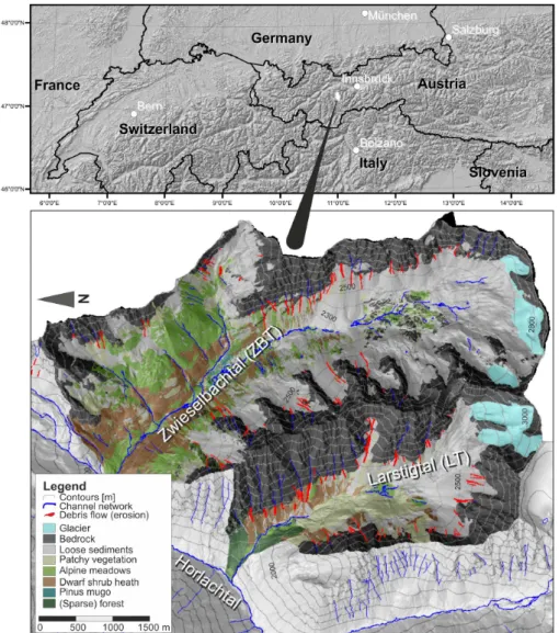
Fig. 1.Overview of the study areas.
The second main goal of this study is to elucidate three aspects of this uncertainty: (i) geofactors and how often they are included after stepwise selection, (ii) the range of model parameters estimated for the replications, and (iii) the spa-tial distribution of differences in the estimated susceptibil-ity. This is important because, in the majority of studies employing sampling for model calculation, only one sam-ple is taken, and no account is given of uncertainty beyond the standard errors of the parameters. On the other hand, most studies involving repeat sampling (e.g. Brenning et al., 2005; Beguería, 2006; Van Den Eeckhaut et al., 2010; Guns and Vanacker, 2012) concentrate on the set of geofactors, the parameters and the predictive ability of the models, and do not investigate how this affects the spatial distribution of susceptibility. Only rarely has the spatial distribution of model uncertainty been addressed using multiple replication approaches (e.g. Guzzetti et al., 2006b; Luoto et al., 2010; Petschko et al., 2014).
2 Study area
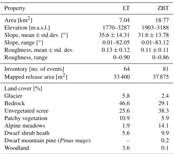
This study has been conducted in two adjacent subcatch-ments of the Horlachtal, a tributary of the Oetztal, located in the Austrian Central Alps (Stubai Alps). The two val-leys, the Zwieselbachtal (ZBT, ca. 19 km2) and the Larstigtal (LT, ca. 7 km2), strike approximately S–N and have a typical trough cross-section. Due to their adjacency, they are simi-lar in their natural characteristics. Figure 1 shows the loca-tion and an overview of the catchments. The most important properties of the study areas are listed in Table 1; the Hor-lachtal and its subcatchments are described in more detail by Rieger (1999) and Geitner (1999).
Table 1.Selected properties of the study areas.
Property LT ZBT
Area[km2] 7.04 18.77
Elevation[m a.s.l.] 1770–3287 1903–3188 Slope, mean±std.dev.[◦] 35.6±14.31 31.6±13.78
Slope, range[◦] 0.01–82.05 0.01–83.12
Roughness, mean±std. dev. 0.13±0.12 0.11±0.11
Roughness, range 0–0.90 0–0.86
Inventory[no. of events] 64 81
Mapped release area[m2] 33 400 37 875 Land cover[%]
Glacier 5.8 2.4
Bedrock 46.6 29.1
Unvegetated scree 25.6 38.3
Patchy vegetation 10.9 5.9
Alpine meadows 1.9 14.1
Dwarf shrub heath 5.6 9.9
Dwarf mountain pine (Pinus mugo) – 0.2
Woodland 3.6 0.1
valley sides, whereas the west-facing valley sides are marked by extensive scree slopes. Currently, the two catchments are formed primarily by fluvial and gravitational processes such as rock falls and debris flows. Sediment transfer through the catchments is limited as the valleys consist of largely disconnected subsystems (at least with respect to the trans-port of coarse sediment; see Heckmann and Schwanghart, 2013) separated by alluvial reaches of the Zwieselbach and Larstig creeks, respectively. These reaches are located im-mediately upstream of the terminal moraines of the Little Ice Age and of the particularly well-preserved terminal moraines of the Egesen stadial (corresponding to the Younger Dryas, ca. 11 to 12 ka BP, recent datings for the European Alps are listed by Ivy-Ochs et al., 2008).
Debris flows in both study areas can be termed slope-type debris flows of slope-type 2 according to Zimmermann et al. (1997). Events of this type initiate on scree slopes follow-ing failure that is caused by positive pore water pressure in the course of intense rainfall, and by progressive erosion. This is often the case at the base of rock walls where debris flow formation is triggered by the so-called “firehose effect” (Johnson and Rodine, 1984) which describes concentrated flux of water out of the rock face onto the talus. Slope-type debris flows can be regarded as a transport-limited process; thus their frequency is primarily controlled by hydroclimatic events (Bovis and Jakob, 1999). In the study area, rain in-tensities of around 20 mm within half an hour have been re-ported to trigger debris flows (Becht, 1995; Rieger, 1999), while Zimmermann et al. (1997) suggest regional intensity-duration thresholds of about 11 mm per hour. The threshold is comparatively low, which has been attributed to the low mean annual precipitation (Hagg and Becht, 2000) of ca. 1000 mm (Becht, 1995).
Vegetation primarily consists of dwarf shrub heath, alpine meadows and pioneer vegetation. At elevations of>2300– 2500 m, bedrock and scree are predominant. In general, more than 60 % of the study area are completely lacking vegetation cover.
3 Data and methods
3.1 Data and data preparation
3.1.1 Debris flow inventory
Like every statistical approach, logistic regression requires an inventory of targets (here: a map of debris flow initiation areas) for the dependent variable, and maps of (potentially) influencing factors as independent variables, hereafter re-ferred to as geofactors. The dependent variable (here: debris flow initiation) is observed as a binary variable (1: presence; 0: absence). The debris flows inventory of the Zwieselbach-tal and LarstigZwieselbach-tal catchment was compiled using orthophoto and field maps (Thiel, 2013), updating an earlier inventory for which debris flows had been surveyed using a total sta-tion (Rieger, 1999). It contains 81 events within the Zwiesel-bachtal and 64 events within the Larstigtal. Debris flows ar-eas are represented by polygon features (which had to be converted to raster format for the pixel-based approach of this study), and divided into three zones related to geomor-phic activity: erosion (indicated by incision), transition (in-dicated by a channelised reach accompanied by levées) and the depositional lobe(s). Conceptually, as the susceptibility map specifically aims at predicting potential initiation zones, the event samples for the regression models should be taken from the erosional zones, preferably from the uppermost part as the latter represents the area where events typically started (and probably will also initiate in the future). The strategy of using only the detachment zone of a mass movement for sus-ceptibility modelling has been advocated by several workers (see for example Van Den Eeckhaut et al., 2006; Heckmann and Becht, 2009); Magliulo et al. (2008), however, report that this restriction does not automatically lead to better results. The initial idea of manually setting one raster cell for each debris flow initiation zone was discarded, because placing this raster cell in the channelised part would introduce a bias towards larger catchment areas and concave plan curvature. Therefore, a GIS procedure was used to select, for each de-bris flow erosional zone, the area that is higher than the P75 percentile of elevation, i.e. the uppermost 25 %. The raster cells belonging to the initiation zone of each debris flows are coded with an ID, allowing for a stratified random sampling of one cell per debris flow event for each regression model.
limiting factor for the reliability of predictive models (e.g. Ardizzone et al., 2002). While fresh landslides are read-ily detected, post-event modifications such as human impact (e.g. ploughing), land cover change, erosion and landslide reactivation etc. can hamper the identification of landslides and thus jeopardise the completeness of the inventory (Bell et al., 2012, e.g., analyse persistence and change of land-slide morphology depending on age). For debris flows in our study area, however, we argue that the risk of false nega-tives, i.e. the risk of an incomplete inventory due to over-looked debris flow scars, is small: the activity of debris flows tends to persist once it has started, because an incision en-hances and sustains the convergence of surface runoff. Due to the transport-limited conditions of debris flow initiation in our study area, this is supposed to hold for a long time, un-til either sediment storage is depleted or slope gradient has become too low. Conversely, debris flow deposits are fre-quently modified by renewed activity, and less pronounced depositional lobes can lose contrast on aerial photos due to progressive weathering (see e.g. Heckmann et al., 2008). Hu-man activities that could potentially modify the appearance of debris flow scars are completely absent in the relevant re-gions of our study area.
3.1.2 Digital terrain model
Before model selection (see Sect. 3.2.2), geofactors concep-tually related to debris flow initiation have been pre-selected. Debris flow initiation is related to (i) the availability of mo-bile debris, (ii) steep slopes, and (iii) large amounts of wa-ter, typically provided by intense rainfall. Not all influenc-ing factors in these three groups (material, relief, water) can be directly measured or calculated; many of them, however, can be derived from a DEM, either directly or as proxies. Although geological and land cover maps were available, we tried to use only geofactors that can be derived from high-quality digital elevation models (DEMs) in order to test the feasibility of DEM-based modelling. Such high-quality DEMs are increasingly available for large parts of the world. For the derivation of several topographical parameters used as geofactors for the regression models, we used a raster DEM with a resolution of 1 m that was interpolated from an airborne lidar survey in the year 2006. For most applica-tions, and for the modelling itself, the original DEM (DEM1) was resampled to a raster resolution of 5 m (DEM5). Apart from saving memory and computing time, the resampling smoothes the DEM so that very fine scale topography is no longer contained in the resulting DEM5. This effect is de-sired, as debris flow initiation is not expected to result from microscale topography.
Information onavailable sedimentis usually provided by land cover and/or geological maps. The former mainly con-tain information on vegetation that might in some cases sta-bilise soils and sediments. The latter focus on different types of bedrock. In this study, the “available sediment” group is
represented by one single geofactor (roughness class). This geofactor is derived from a cluster analysis of slope (DEM5; see below) and roughness. Roughness was calculated as the “vector ruggedness measure” (Sappington et al., 2007) on the DEM1 within a moving window of radius 5 m, and the result was resampled to the same resolution and extent as the DEM5 using the nearest-neighbour approach. The com-paratively small radius was chosen to capture the rough-ness of surfaces rather than the roughrough-ness induced by land-forms, e.g. by gullies. The cluster analysis yields two clus-ters closely representing (i) bedrock and (ii) areas covered by sediments. For the Zwieselbachtal, this unsupervised classi-fication could be validated with a very detailed land cover map created from orthophoto imagery; theφ coefficient of the mapped vs. the DEM-based classification was 0.78. The reason for the satisfactory fit is the characteristic fine-scale roughness2of bedrock areas that can easily be discerned on a shaded relief map, together with the existence of a sharp threshold of slope (resembling the angle of internal friction) above which an area cannot be covered by unconsolidated scree. Leaving out the information on land cover/vegetation is not expected to be decisive in our case study, because the study areas are only sparsely covered with vegetation, mostly grass, and forest is widely missing, at least in the areas rele-vant for debris flow genesis.
Relief parameterswere derived from the DEM5 using the
algorithm of Zevenbergen and Thorne (1987) implemented in SAGA GIS (www.saga-gis.org). As slope stability, espe-cially for scree, is a function ofslope, this parameter is ex-pected to be very important for debris flow initiation. As both valley axes have a north to south orientation (resulting in a strong bias towards east- and west-facing slopes), and as the physical role ofaspect cannot be described unambigu-ously, it was not included in the analysis. Plan and profile
curvatures were derived with the same algorithm as slope,
but from a DEM5 smoothed with a moving window mean filter with a radius of 10 m. This was deemed necessary be-cause of the extremely noisy character of fine-scale curva-ture. Medium-scale curvature based on a DEM that retains details on the typical spatial scale of channels within the rock faces and talus cones (that are both prone to and indicative of debris flow activity) is expected to be a better proxy variable for convergent flow of water (plan curvature) and changes in flow velocity (profile curvature).
Relief parameters related to the local catchment area are derived from the DEM5 as proxies for the availability of
water for debris flow initiation. We calculated the specific
catchment area (SCA) as the local flow accumulation per
overland flow; on talus slopes bordering steep rock faces, this runoff can cause the initiation of debris flows, especially where it enters the talus in a channelised manner (“firehose effect”; see e.g. Johnson and Rodine, 1984; Coe et al., 2008). However, if the sediment is coarse grained, large amounts of water are expected to infiltrate; this leads to a decrease of hydrological connectivity, and at least to an attenuation of the increase of runoff with increasing catchment size. There-fore, we re-calculated the catchment area, accumulating only bedrock cells in the roughness class map instead of every DEM5 raster cell. The modified SCA map hence refers to the size of the bedrock catchment draining into each raster cell.
3.2 The susceptibility model
Multivariate logistic regression (Hosmer and Lemeshow, 2000) forms part of the family of generalised linear models (GLMs); in contrast to ordinary linear models, a function of the expected value of a response variable is modelled by a linear combination of continuous or discrete predictor vari-ables. In logistic regression, the response variable is binary (Bernoulli distribution); here, it takes the values 0 (no debris flow initiation) and 1 (debris flow initiation). The response function is the logit transform of the probabilityp∈ ]0,1[
that the response variable takes the value 1:
f (p)=logit(p)=ln p
(1−p). (1)
Since the logit is within the interval ] − ∞,∞[, it can be modelled as a linear combination of predictor variables X1. . . Xn:
f (p)=β0+β1x1+β2x2+. . .+βnxn, (2)
whereβ0 is the intercept and β1 . . . βn are the model pa-rameters. These are estimated using a maximum likelihood approach.
The spatial data are generated and managed in SAGA GIS, including the derivation of relief parameters (Sect. 3.1.2); for the statistical analysis, they can be directly read from the SAGA native data format using the RSAGA package (Brenning, 2013) for the statistical software R (R Devel-opment Core Team, 2012). Logistic regression is then per-formed using the glm and stepAIC functions of the MASS package (Venables and Ripley, 2002). For reasons explained in the Introduction, we estimate the model parameters for a sample (the size of which we will try to optimise in this study) of event (debris flow initiation) and non-event cells; sampling is also performed in R. The resulting susceptibility maps are written back to SAGA data format for visualisation and further spatial analysis. They contain the probability that the dependent variable takes the value 1, i.e. that debris flow initiation will take or has taken place.
3.2.1 Multicollinearity analysis
Besides sample independence, an important prerequisite for the application of GLM is the absence ofmulticollinearity, i.e. that the predictor variables are not correlated with each other. In order to test for multicollinearity, we applied the vif function of the car package (Weisberg and Fox, 2010) to a full model (i.e. including all geofactors described in Sect. 3.1), yielding the variance inflation factors (VIF) of each geofactor. Although no binding rules exist for their in-terpretation, several authors who conduct a multicollinearity analysis apply a very strict threshold of 2, above which vari-ables are considered multicollinear and are excluded from the model (e.g. Van Den Eeckhaut et al., 2006, 2010; Guns and Vanacker, 2012). However, the most common rule of thumb is reported to be the “rule of 10” (using VIF = 10 as a threshold for severe multicollinearity), and the use of strict thresholds of VIF appears to be questionable (O’brien, 2007). The analysis of VIFs yields values of 1.18 and 1.47 for the two curvature variables, and 1.77 for SCA. Roughness and slope have VIFs of 2.06 and 2.76, respectively, which is only slightly above the threshold used in other studies, so we de-cided to keep all candidate variables.
3.2.2 Stepwise selection of predictor variables
An important task in susceptibility modelling is model build-ing, i.e. theselection of the independent variables (geofac-tors). In Sect. 3.1, several candidate variables are described that conceptually explain the spatial distribution of debris flow initiation. Model building is achieved in this study through an automatic stepwise variable selection (function stepAIC; Venables and Ripley, 2002). Starting from a full model, i.e. a model including all variables, variables are re-moved (or re-included) in order to minimise the Akaike in-formation criterion (AIC; Akaike, 1973) which is calculated from the likelihood function of the model and the number of predictor variables. The AIC penalises for the number of predictor variables; i.e. it increases with the number of vari-ables, and it decreases with a larger likelihood function indi-cating a better model. Hence, although there is no theoretical justification of the AIC (Sachs and Hedderich, 2006), this procedure is suitable in practice for selecting a parsimonious model, i.e. a best-fit model using as few variables as possible (Brenning, 2005). The results of stepwise logistic regression have often been used to rank the controlling factors by im-portance (e.g. Van Den Eeckhaut et al., 2006). While we as-sume that the methodological framework of our study would also be suitable for the assessment of sample size effects in such investigations (Guns and Vanacker, 2012, e.g., suggest a “robust detection of controlling factors” based on repeated sampling and stepwise model selection), the latter are not the aim of our present study.
et al., 2011), but also as a forward selection (Beguería, 2006; Meusburger and Alewell, 2009; Atkinson and Massari, 2011). Menard (2002) explains that backward selection is in some cases superior to the forward procedure. Note that the stepwise procedure used here and in Brenning (2005) differs from other studies where the decision of keeping or drop-ping predictor variables is based on the significance of model improvement (e.g. Beguería, 2006; Meusburger and Alewell, 2009; Guns and Vanacker, 2012), not on an information cri-terion. Recently, alternative approaches for model selection have been proposed (e.g. Calcagno and Mazancourt, 2010); they will be tested in future research.
3.2.3 Model validation
It has been stressed that a modelling study without proper validation is useless (Chung and Fabbri, 2003). Many stud-ies in susceptibility modelling use spatial or temporal cross-validation (space or time partition; cf. Chung and Fabbri, 2003) within the same study area; i.e. the data are split ei-ther systematically or randomly into training and test data sets according to their location or time of occurrence (Chung and Fabbri, 2003; Beguería, 2006). Here, we estimate model parameters based on samples drawn from the Zwieselbachtal catchment, and apply the resulting models to the neighbour-ing Larstigtal catchment. Hence, trainneighbour-ing and test areas are completely independent. For each model run, the predictive ability is evaluated using receiver operating curves (ROCs) or prediction-rate curves sensu Chung and Fabbri (2003), plot-ting true-positive against false-positive rates. The advantage of ROCs is that they yield a threshold-independent measure of predictive ability; in our case, we do not have to define a threshold of modelled landslide probability below which we do not recognise susceptibility. Additionally, as a single mea-sure of predictive ability, the AUC is calculated (Hosmer and Lemeshow, 2000; Beguería, 2006); this parameter falls in the range [0.5, 1], where 0.5 is equivalent to random prediction and 1 to a perfect prediction.
3.3 Exploring the effect of sample size
In the Introduction, we have argued why the sample size should be neither too small nor too large. Here, we describe (i) how the effect of sample size on the diversity of models is explored, and (ii) how we constrain the upper limit of sample size.
3.3.1 Sample size and model diversity
For small sample sizes, the geofactor composition of the resulting model depends extremely on the random sample, because small samples cannot sufficiently cover the diver-sity of geofactors within the study area. We hypothesise that with increasing sample size the diversity of relevant models (selected by the stepwise procedure) first decreases towards a plateau that can be explained with the overall variability
of geofactors in the study area; when the sample size ap-proaches the size of the study area, the variability of models will eventually decrease to zero. Such a behaviour is similar to the dependence on sample size of the predictive power of predictive geomorphological models that has been explored by Hjort and Marmion (2008).
We analyse model diversity by repeating the stepwise model selection with 1000 independent samples of a given sample size. Such a high number of replications is novel compared to existing studies that employ multiple sam-ples; we chose the number of 1000 because we noticed in first experiments that the model diversity assessment was too unstable with a lower number of replications (e.g. be-tween 25 and 50 in the studies of Brenning, 2005; Beguería, 2006; Guns and Vanacker, 2012). Sample size varies between n= 50 andn= 5000 non-event raster cells; together with the sample ofn=81 initiation areas in the ZBT area, the sam-ples cover between 0.02 and 0.68 % of the study area (ZBT). Specifically, a stratified sampling scheme has been adopted; one single raster cell is randomly selected from each debris flow initiation zone, and the sample size of non-event cells (from the area outside of the mapped initiation zones) is var-ied. The choice of non-event sample sizes in relation to event sample size ranges from ca. 1 : 1.6 to ca. 60 : 1, thus including the recommendations of King and Zeng (2001) and the al-ternatives chosen in landslide susceptibility studies, e.g. 5 : 1 (Van Den Eeckhaut et al., 2006) or 10 : 1 (Beguería, 2006; Guns and Vanacker, 2012).
For each of the 1000 samples, the geofactors that remain in the “best” model (with respect to the AIC) after stepwise selection are saved in a table. Each geofactor is evaluated by the percentage of models which it was part of (cf. Guns and Vanacker, 2012). The set of selected geofactors for one sam-ple defines a “model species” (if, for examsam-ple, the geofac-torsA,BandDare selected from the candidate geofactorsA,
B, . . . E, the species of the resulting model is ABD). The
term model species was used in order to highlight the simi-larity of the proposed method for model diversity assessment with investigations of biodiversity in ecology. Theoretically, kmax= 2g−1 different model species can exist ifgcandidate geofactors are available for model selection, and if the result-ing model has to contain at least one geofactor. The diversity of the 1000 replicate models calculated for each sample size is evaluated using three measures: (i) the numberk of dif-ferent model species (“species richness”); (ii) the Shannon diversity indexH, also known as Shannon information en-tropy; and (iii) the Simpson indexD.
H = − k X
i=1
pi ·ln(pi) , (3)
where i= 1 . . . k represents the ith of k different model species, and pi is the probability of occurrence of the ith species, estimated byni/N, the proportion of theith model species found inNindividual stepwise modelling runs.
The log-transformed Simpson index (Simpson, 1949) has been developed for measuring biodiversity; it is consid-ered superior to the H as it is independent of sample size (Magurran, 2004). It is calculated as
D= −ln
k X
i=1
ni ·(ni −1)
N ·(N−1), (4)
whereni is the absolute frequency of theith model species andN is the number of individual models (here: 1000).
H andDcombine the number of different model species (species richness) and their relative frequency (relative “abundance”) in one single number: a large diversity asso-ciated with a high species richness (k different terms have to be summed up forHandD, respectively) and/or an even distribution of model species across the 1000 samples. Con-versely, diversity is low when there is only a small number of different species, and/or one or few species strongly dom-inate. Shannon’s entropy has been interpreted in terms of the “average surprise a probability distribution will evoke” (see e.g. Thomas, 1981, p. 7). The result of a stepwise selection with a sample size for which low diversity (lowH) has been measured is not expected to be surprising, because one or few species have a very high probability of occurrence. We hypothesise that the diversity of model species, and the de-gree of surprise with which we see one particular outcome of the selection given the results of 1000 models, will re-flect the sample dependence of the stepwise selection. There-fore, we propose the “model diversity” as a measure of model quality in terms of reproducibility; similarly, Petschko et al. (2014) recently proposed a “thematic consistency” index that assesses variable-selection frequencies in model replications and is based on the Gini impurity index.
3.3.2 Sample size and spatial autocorrelation
In our study, the spatial autocorrelation of a data set is ex-plored with the empirical semivariogram, which is typically used for geostatistical interpolation techniques such as Krig-ing (Webster and Oliver, 2007). It is derived from point mea-surements by evaluating the semivariance of values of a vari-able (geofactor) for pairs of points separated by a specific distance. One important property of the semivariogram is the range; points separated by a distance below this range are au-tocorrelated. Brenning (2005) uses the range of the empirical correlogram of the residuals of a logistic regression model (180 m in his study) to constrain the minimum distance be-tween training and test data points in spatial cross-validation.
Similarly, we estimate the range parameter of the variogram of each geofactor to constrain the sample size: we argue that the average distance between raster cells in the (non-event) sample should not fall within the autocorrelation range(s) of the geofactors included in the model in order to keep the non-event sample as uncorrelated or independent as possible. As the average distance implies that some points in the sample will be closer neighbours, we concede that this strategy min-imises spatial autocorrelation rather than preventing it.
Assuming a set of randomly distributed points (here: raster cells), the average distancedˆto the nearest neighbour can be estimated by Eq. (5):
ˆ
d = 1
2·√ρ, (5)
(Clark and Evans, 1954) whereρis the density of the sam-ple, i.e. the sample sizen divided by the study area (here: the number of raster cells within the study area multiplied by 25 m2, the area of each cell). For each study area,dˆ is calculated as a function ofnand used to estimate the upper boundary for the “suitable sample size”. Instead of using the highest autocorrelation range (i.e. that of the geofactor with the most far-reaching spatial autocorrelation) as a crisp, ab-solute upper limit of sample size, we take into accountd(n)ˆ as it progressively falls below the autocorrelation range of more and more geofactors, and we regard the corresponding nas progressively less acceptable. An upper limit is finally reached when the smallest autocorrelation range from the set of geofactors is undercut.
Figure 2 shows the empirical geofactor semivariograms and the practical range parameter (i.e. the range where 95 % of the sill is reached) of the fitted variogram models. Depend-ing on the geofactor, spherical and exponential models were used. It is obvious that some geofactors, e.g. slope, are auto-correlated on multiple scales. In these cases, the lower range is used; however, it appears that a sample which is indepen-dent with respect to all geofactors is not possible.
3.4 Variability of model results
P
❛♣
❡r
⑤
❉✐s❝✉ss✐♦♥
P
❛♣
❡r
⑤
❉✐s❝✉ss✐♦♥
P
❛♣
❡r
⑤
❉✐
s❝✉ss
✐♦♥
P
❛♣
❡r
⑤
Fig. 2.Empirical variograms of geofactors used in this study. Note
that slope is autocorrelated at different spatial scales.
As this measure is calculated for each raster cell, the respec-tive map can be used to visualise the spatial distribution of model uncertainty (not with respect to the true probability, but with respect to model variability). In addition, the distri-bution of the parameter coefficients of the 100 models, and their predictive power (ROCs and AUC; see Sect. 3.2.3) can be displayed and analysed.
4 Results and discussion
4.1 Investigation of sample size effects
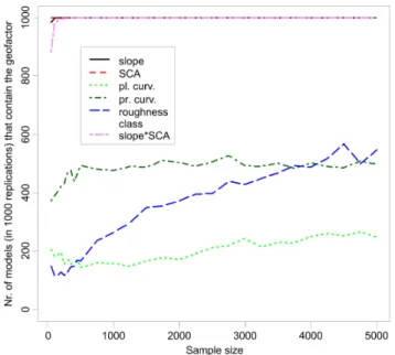
Before we approach the question of an optimal range of sample sizes, we take a look at the results of model se-lection as a function of sample size. Specifically, Fig. 3 shows, for each geofactor, the number of models that retained this geofactor after the AIC-based selection procedure. The six geofactors that were eligible for model selection were slope, SCA, the interaction of the previous two factors (de-noted “slope*SCA” in Fig. 3), the roughness category which
❉✐s❝✉ss✐♦♥
P
❛♣
❡r
⑤
❉✐s❝✉ss✐♦♥
P
❛♣
❡r
⑤
❉✐s❝✉ss✐♦♥
P
❛♣
❡r
⑤
❉✐
s❝✉ss
✐♦♥
P
❛♣
❡r
⑤
Fig. 3.Overview of the six geofactors and their contribution to
1000 models of different sample sizes. The y axis denotes the number of models for which the respective geofactor was selected. “slope*SCA” signifies the interaction term of the two variables slope and specific catchment area.
distinguishes bedrock from debris-mantled slopes, and the two curvature variables. While roughness and profile curva-ture gradually increase their membership with larger sample sizes (roughness starting from only ca. 15 % of the replica-tions), the interaction term slope*SCA quickly attains 100 % (i.e. all of the 1000 samples lead to models containing this variable) even with small samples. Here, it is important to mention that interaction terms may only be part of a model if their marginals (here: slope and SCA) are also contained. This is the case, as the given variables are contained in all models, irrespective of sample size. The proportion of mod-els containing the geofactor plan curvature is very low, start-ing with about 20 % and only slightly increasstart-ing in larger samples.
the compound topographic index indicating stream power (Moore et al., 1991); in this index, catchment area and slope serve as proxies for the abundance and energy of surface runoff. In comparing several models (discriminant analy-sis and logistic regression) Carrara et al. (2008) observed that factors relating to slope gradient, land cover, availabil-ity of detrital material, and active erosional processes best described debris flow initiation. The most frequent model species in our study include geofactors that represent these categories.
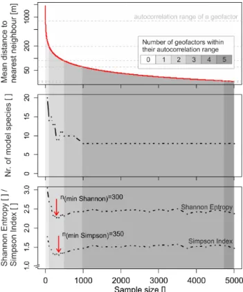
Figure 4 evaluates the diversity of models selected by the AIC-based procedure as a function of sample size. The diver-sity is expressed as the number of model species (i.e. models defined by a given combination of geofactors) in 1000 sam-ples (centre panel), and is quantified using the Shannon and Simpson diversity measures (bottom panel). The number of model species declines exponentially to reach a stable min-imum of 8 species at a sample size ofn= 1000. Even for the largest sample size in our analysis (n= 5000), differences between the 1000 samples result in as many as 8 different model species. The diversity measures show a local mini-mum atn= 300 andn= 350, respectively; for these sample sizes (nrel= 0.05 %), the number of model species is higher, but the distribution of the 1000 models across this number of species is more uneven – i.e. few species make up the lion’s share of the selections – and the rest is represented only by a few cases. For larger sample sizes, model diversity slightly increases again and reaches a more or less stable value. Sam-ple sizes much larger than 5000 (nrel>0.68 %, not shown) lead to a decrease of the diversity indices; when the sample size approaches the size of the population (i.e. the complete study area), the stepwise procedure of course yields only one model species, and the diversity indices attain their absolute minimum (0). The plateau of the diversity measures is also reflected in the model composition shown in Fig. 3 where all geofactors (except roughness) exhibit only slight changes with sample sizes larger than ca. 1000 (nrel= 0.15 %).
We interpret the minimum of the diversity indices as a minimum of the dependence of model selection on the sam-ple and therefore the corresponding samsam-ple size (300–350) as a data-based recommendation for our case study. Such a strategy is, in our opinion, better than the adoption of arbi-trary recommendations with respect to event : non-event ra-tios, absolute, or relative sample sizes. The sample size of 300–350 event cells corresponds to a ratio of event : non-event of 1 : 3.7 to 1 : 4.3, which is approximately consistent with the 1 : 5 ratio used by Van Den Eeckhaut et al. (2006) and with the recommendation (1 : 2–1 : 5) given by King and Zeng (2001). It is also in the range of the ratio of event to non-event cells in our study areas (about 1 : 500 in ZBT, 1 : 200 in LT), a ratio that has been used by Atkinson et al. (1998). Considering Green’s rule of thumb (Green, 1991) re-ported in the Introduction (Sect. 1.1), the six candidate geo-factors in our case study would require a minimum sample size of ca. 100. Hjort and Marmion (2008), who investigate
P
❛♣
❡r
⑤
❉✐s❝✉ss✐♦♥
P
❛♣
❡r
⑤
❉✐s❝✉ss✐♦♥
P
❛♣
❡r
⑤
❉✐
s❝✉ss
✐♦♥
P
❛♣
❡r
⑤
Fig. 4.Mean distance between neighbouring sample points (top
panel), number of model species in 1000 samples (center panel), and two model diversity measures (bottom panel) as a function of sample size. Shades of grey denote the degree to which the raster cells in a sample of size n lie, on average, within the autocorrela-tion range of geofactors. Red arrows indicate the sample sizes for which the Shannon and Simpson indices reach a local minimum, respectively.
the predictive power of different models estimated with dif-ferent sample sizes, state that a “level of robust predictions” is attained, with all statistical techniques, at a sample size of n= 200.
T. Heckmann et al.: The effect of sample size on a debris flow susceptibility model P❛♣ 271
❡r
⑤
❉✐s❝✉ss✐♦♥
P
❛♣
❡r
⑤
❉✐s❝✉ss✐♦♥
P
❛♣
❡r
⑤
❉✐
s❝✉ss
✐♦♥
P
❛♣
❡r
⑤
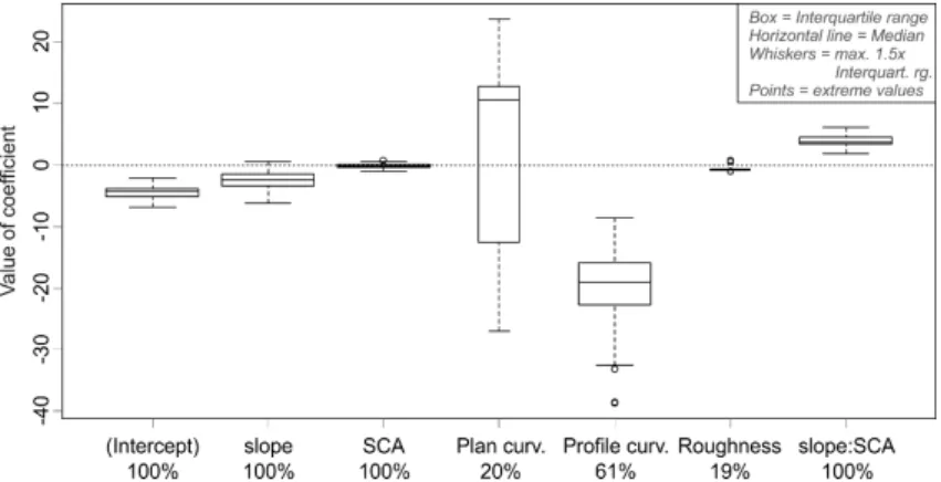
Fig. 5.Distributions of model coefficients estimated from 100 random samples (n= 350 non-event cells) in the ZBT area. The percentages
below the parameter name refer to the proportion of the 100 models that contain the respective geofactor.
open to future research, employing a systematic analysis of multiple study areas with different sizes, characteristics, and debris flow densities.
In Sect. 3.3.2, we proposed the mean distance between sampled locations in relation to ranges of spatial autocorre-lation as an upper constraint of sample size. Figure 4 (top panel) shows the expected mean distance between nearest neighbours as a function of sample size (see Sect.3.3.2). Ad-ditionally, the horizontal dashed lines indicate the autocorre-lation ranges of the geofactors mentioned above (cf. Fig. 2). As the red curve intersects the autocorrelation ranges of more and more geofactors, the sample of the corresponding size is more and more likely to violate the independence assump-tion. The decreasing suitability of larger samples to this end is visualised across the whole Fig. 4 through darker shades of grey. The optimal sample sizes indicated by the red arrows in the bottom part of the diagram belong to a range of sample sizes that are within the autocorrelation range of one single geofactor only. In this case, it is the “large-scale” range of slope (ca. 800 m, slope is autocorrelated also at smaller spa-tial scales with a range of ca. 200 m; see Fig. 2). We consider this only a minor violation of the independence assumption, so that the sample size recommended above remains optimal also with respect to the spatial autocorrelation issue that has been raised in Sect. 1.2.
While the typical scale of application of landslide suscep-tibility models is in the order of (many) tens to thousands of square kilometres, our study took place in a comparatively small study area. Considering the small size and the associ-ated homogeneity of our study area with respect to the sta-tistical and spatial distribution of geofactors, we add a note of caution to the interpretation of our findings. First, we ex-pect the necessary sample size to be larger in more hetero-geneous areas, and we expect a larger variability of model selection and model coefficients. One possibility of dealing with large, heterogeneous study areas has recently been pro-posed by Petschko et al. (2014), who partition their study area in sub-areas based on lithological properties that are
related to landslide activity. Second, the assessment of spatial autocorrelation from variograms of the geofactors is much less straightforward in larger, heterogeneous areas. For ex-ample, different ranges of autocorrelation could exist for the same geofactor in different (sub-)regions of the study area, which calls into question the existence of a single sample size (and the associated average distance between sample points) below which the autocorrelation issue is mitigated. However, we are confident that our observation of a local minimum or plateau in model diversity will apply also at larger spa-tial scales (see, for example, Hjort and Marmion, 2008; Guns and Vanacker, 2012). Moreover, we uphold the general rec-ommendation to investigate, through repeated sampling with different sample sizes, the behaviour of parameter selection in order to explore a suitable (small) sample size that both minimises sample dependence and facilitates a robust param-eter selection.
4.2 Model results
4.2.1 Model parameters
from the upper erosional zones in the debris flow inventory will select locations not only in the centre of channelised de-bris flow paths (with highly concave plan curvature) but also at the boundary of these areas, which are highly (plan) con-vex. Conversely, the profile curvature coefficient is strictly negative, which means that a concavity in the long profile increases the probability of debris flow initiation. The ex-planation for this finding is a morphological one: the typi-cal locations of debris flow initiation (facilitated by the fire-hose effect; see Fig. 1) at the contact of steep rock faces and the corresponding talus cones are marked by large negative (i.e. concave) profile curvatures.
The mostly negative coefficients for slope and SCA are difficult to interpret, as one would expect that the proba-bility of debris flow initiation would increase with steeper slopes and with larger catchment areas. However, this prob-lem appears to be only a mathematical one, as the interac-tion term of slope and SCA is present in the model. There-fore, the coefficient of slope (alone) models the effect of slope where SCA is zero (and vice versa); the coefficient for the interaction term is positive, indicating higher proba-bilities with steep slopes and large catchment areas, which is conceptually correct. The interaction term plays an im-portant role in the model: without it, the positive relation-ship of SCA with debris flow release causes the modelled susceptibility to increase even in the comparatively flat val-ley bottoms. Under these conditions, slope-type debris flows cannot occur; Rickenmann and Zimmermann (1993) report starting zone slopes for type 2 debris flows (that type which occurs in our study areas) between 26.5 and 38◦, with catch-ment sizes of up to 1 km2; Takahashi (1981) gives a lower threshold for debris flow initiation of 15◦. Generally, there appears to be a trend that the minimum slope angle required for debris flow release decreases with larger catchment ar-eas (Rickenmann and Zimmermann, 1993; Heinimann et al., 1998; Horton et al., 2008), so there is, besides the stream power index (cf. Sect. 4.1), one more theoretical justification for including the interaction of slope and SCA.
4.2.2 Susceptibility maps
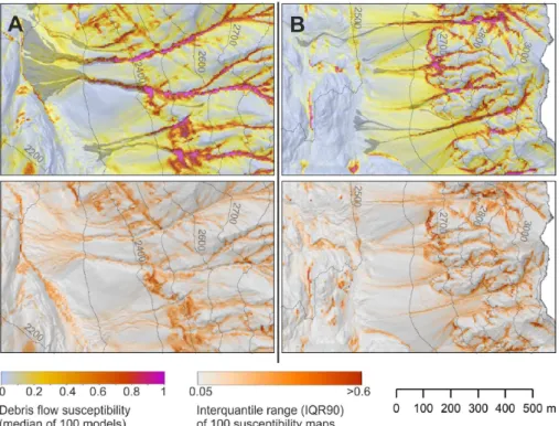
The previous analyses have shown the dependence of mod-els found through AIC-based model selection on the respec-tive sample and its size. The spatial pattern of a model re-sult (here: the susceptibility map containing the debris flow initiation probability) depends on the spatial pattern of the geofactors that form part of the model. Figure 6 shows a sec-tion of the susceptibility map that can be seen as a consensus model (see Marmion et al., 2009) as every raster cell con-tains the median of 100 model predictions, the coefficients of which have been summarised in the previous section (Fig. 5). Susceptibility in both valleys has been predicted using the model estimated with ZBT data only. The whole map is part of the supplementary material of this paper. On the map, de-bris cones are highlighted by yellowish to reddish colours
Fig. 6.Part of the susceptibility map (for full extent, see
Supple-ment) of the ZBT and LT areas. The susceptibility values represent a model ensemble, specifically the median value of 100 models es-timated from 100 random samples (n= 350 non-event cells) in the ZBT area. Insets A and B refer to map sections in Fig. 7.
Fig. 7.Map sections (for full extent, see Supplement) from the ZBT(B)and LT(A)areas. The maps show the susceptibility map (see Fig. 6) and a map of the IQR90 calculated from the model ensemble. The latter map represents the uncertainty of the susceptibility map that is due to the sampling process.
the aerial photo. Second, a linear modelling approach is not capable of modelling complex non-linear relationships such as the one of slope and debris flow release: conceptually, susceptibility should increase, starting from some minimum slope, up to a maximum and then decrease again. The sus-ceptibility then reaches zero at slope gradients that are pro-hibitive for the formation and persistence of sediment stor-age that is needed for debris flow generation. The GLM ap-proach, however, only handles monotonic relationships be-tween independent and dependent variables, e.g. an increase of susceptibility with slope. Problems of this kind could be solved by using other approaches, for example the weights of evidence, certainty factor, or generalised additive models (GAM; see e.g. Hjort and Luoto, 2011).
A novel output of our model replication exercise is the quantification of the variation in model results and the as-sessment of its spatial distribution. The model uncertainty addressed here is due to the sampling and model selection procedure only. For each raster cell of the susceptibility map, we computed not only the median but also the interquan-tile range (IQR90) between thep0.95andp0.05quantiles; the corresponding map can be seen in the supplementary ma-terial and in Fig. 7, bottom row. In the whole study area, the IQR90 has a highly positively skewed distribution that ranges from 0.0 to 0.98. It has a mean of 0.081; i.e. debris flow release probability predicted by the 100 models varies by 8 percentage points, on average. In the ZBT area (that
was used to estimate the models) this value equals 0.073, while in the LT area it is slightly higher (0.103). For sam-ples taken according to the “1 : 1 event to non-event” rule (n= 81 non-event cells,nrel= 0.022 %), the average IQR90 is 0.190 (ZBT), 0.230 (LT) and 0.200 (total study area). The expected variability is consistently higher for smaller sam-ples, and when a model is applied to a different area. The lat-ter can be explained with the effect of extrapolation beyond the range of geofactors in the respective training area.
274 T. Heckmann et al.: The effect of sample size on a debris flow susceptibility model
4.2.3 Validation
The variability of model parameters and predictions is also reflected in the validation. A first qualitative validation is done by visually inspecting the susceptibility map (here: the median of 100 models, Figs. 6 and 7). Each model is quan-titatively validated by means of a ROC (see Sect. 3.2.3) us-ing data from the Larstigtal (LT) only; hence, the data used to estimate the model parameters (from the ZBT area) and the validation data are completely independent, and the cor-responding diagram represents a “prediction curve” (Chung and Fabbri, 2003). Split-sample validation approaches such as cross-validation, spatial and temporal partitions (Chung and Fabbri, 2003) do not warrant such independence when, for example, subsets of the same inventory are used to esti-mate model parameters and to validate the resulting model in one study area.
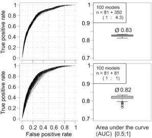
Figure 8 (top panels) shows the prediction curves for the 100 models, and the distribution of the corresponding area under the curve (AUC). The 100 curves are located quite close to each other, and there are no conspicuous extreme outliers. The AUC reaches 0.83, on average; the predictive ability of a model calculated in the LT area and applied to the ZBT (not shown) is even higher, with AUC = 0.9. In total, the observed AUCs are within the range of many published studies (e.g. 0.69–0.8: Ruette et al., 2011; 0.84: Ayalew and Yamagishi, 2005; 0.89–0.93: Van Den Eeckhaut et al., 2010) and can be regarded as satisfying. The different performance of the ZBT model in the LT area and vice versa is an interest-ing fact. This could be caused by different characteristics of the study areas, related to a different range, and different spa-tial and statistical distributions of the geofactor values. The two neighbouring areas, however, are regarded as very sim-ilar and homogeneous. Heckmann and Becht (2009) investi-gated the transferability of a debris flow susceptibility model among different study areas and reported that the predictive power of models is largely independent of the degree of sim-ilarity of training and test area; their model approach (cer-tainty factor), however, strongly differs from logistic regres-sion. Besides computational and conceptual differences, con-tinuous geofactors such as slope are classified using the same scheme in all study areas. Conversely, in our study, a differ-ent range of geofactors in training and test areas could lead to different coefficients and different model performance due to extrapolation. Another reason for the different performance could be the different debris flow density. In order to deter-mine the controls of model performance, future research will have to use a larger number of different study areas with dif-ferent debris flow densities. The methodological framework for the assessment of model variability and performance pro-posed here is considered useful for such investigations.
Interestingly, the sample size did not influence the predic-tive ability of the model ensemble – bothn= 81 andn= 350 have very similar mean AUC values. However, the smaller sample size leads to a much larger spread of the different
P
❛♣
❡r
⑤
❉✐s❝✉ss✐♦♥
P
❛♣
❡r
⑤
❉✐s❝✉ss✐♦♥
P
❛♣
❡r
⑤
❉✐
s❝✉ss
✐♦♥
P
❛♣
❡r
⑤
Fig. 8.Evaluation of the predictive ability of 100 models (top
pan-els:n= 350 non-event cells, bottom panels:n= 81 non-event cells) by means of the area under the curve. As the model training (ZBT) and validation area (LT) are independent, the diagrams on the left represent prediction curves (Chung and Fabbri, 2003).
prediction curves and consequently also of the AUC values. In our case, a single sample of events and non-events at a ra-tio of 1 : 1 (see, for example, Brenning, 2005; Meusburger and Alewell, 2009) could have resulted in a good model (AUC 0.84) but also in a comparatively poor one (AUC 0.75), although the expected AUC is approximately the same. We deduce from our results a recommendation to create sus-ceptibility maps from model ensembles, because they are supposed to yield a more reliable result on the one hand and give an estimation of (sample-induced) uncertainty on the other. Similarly, Marmion et al. (2009) propose “con-sensus models”; in their study, results from different predic-tive modelling approaches are combined using several meth-ods, among them the median that was used in our study to combine the results of 100 models generated with the same method, but from independent random samples.
5 Conclusions
In this paper, we investigated the effect of sample size on a logistic regression model with a parameter selection proce-dure that is based on an information criterion (AIC). The case study aims at predicting the spatial distribution of slope-type debris flow release zones in the Larstigtal (LT) and Zwiesel-bachtal (ZBT) catchments in the Austrian Central Alps.