http://dx.doi.org/10.4236/jamp.2014.23004
Numerical Uncertainty and Its Implications
António F. Rodrigues1,2, Nuno O. Martins1,31
Campus de Angra do Heroísmo, University of the Azores, Angra do Heroísmo, Portugal 2
CITA-A, Angra do Heroísmo, Portugal 3
CEGE, Porto, Portugal Email: [email protected],[email protected]
Received December 10, 2013; revised January 10, 2014; accepted January 17, 2014
Copyright © 2014 António F. Rodrigues, Nuno O. Martins. This is an open access article distributed under the Creative Commons Attribution License, which permits unrestricted use, distribution, and reproduction in any medium, provided the original work is properly cited. In accordance of the Creative Commons Attribution License all Copyrights © 2014 are reserved for SCIRP and the owner of the intellectual property António F. Rodrigues, Nuno O. Martins. All Copyright © 2014 are guarded by law and by SCIRP as a guardian.
ABSTRACT
A scrutiny of the contributions of key mathematicians and scientists shows that there has been much controversy (throughout the development of mathematics and science) concerning the use of mathematics and the nature of mathematics too. In this work, we try to show that arithmetical operations of approximation lead to the existence of a numerical uncertainty, which is quantic, path dependent and also dependent on the number system used, with mathematical and physical implications. When we explore the algebraic equations for the fine structure constant, the conditions exposed in this work generate paradoxical physical conditions, where the solution to the paradox may be in the fact that the fine-structure constant is calculated through different ways in order to ob-tain the same value, but there is no relationship between the fundamental physical processes which underlie the calculations, since we are merely dealing with algebraic relations, despite the expressions having the same physi-cal dimensions.
KEYWORDS
Geometry; Algebra; Numerical Uncertainty; Fine Structure Constant and Physical Uncertainty
1. Introduction
In this article, we study the implications of numerical uncertainty for the measurement of various physical mag-nitudes, such as the fine-structure constant and the speed, mass and charge of an electron. Numerical uncertainty occurs due to the need to engage in processes of algebraic approximation, and has profound implications for the measurement of physical magnitudes, which have been relatively neglected in the study of the relationship be-tween mathematics and sciences such as physics.
The use of mathematics in science became so widespread that it is now difficult to imagine the formulation of scientific theories in many areas, such as physics, without the use of mathematics. Mathematics brought preci-sion to the formulation of many theories within astronomy, and within the natural sciences, especially when there is the possibility of insulating causal mechanisms within an experimental context.
Given the widespread success of the use of mathematics as an instrument for formulating scientific theories, there has not been much scrutiny of the nature of the instrument which contributed so much to this success. Ma-thematics is taken to be a standard of precision, and an instrument which brings precision to the formulation of scientific theories.
However, a scrutiny of the contributions of key mathematicians and scientists shows that there has been much controversy throughout the development of mathematics and science, concerning the use of mathematics, and the nature of mathematics too. And a careful investigation of those controversies has important implications for the interpretation of scientific theories. For it shows that the instrument which is taken to be a standard of preci-sion, namely, mathematics, has not always been used with full precipreci-sion, a fact which introduces much
uncer-tainty in the numerical estimations made within scientific measurement, and in the very formulation of scientific theories.
We start the article with a brief discussion of the use of geometrical and algebraic methods within mathemat-ics, and afterwards address the implications of the use of those methods within scientific studies. We then show the implications of the use of algebraic or numerical approximations, and their path-dependent nature. Those implications are then scrutinized in more detail in the case of physics, more specifically when measuring the fine-structure constant and the relationship between the mass, speed and charge of an electron.
2. Geometry and Algebra
The mathematician Michael Atiyah [1] notes that behind the controversy between Newton and Leibniz over dif-ferential calculus, there were two mathematical traditions, one grounded on geometry, which Newton followed, and another one dealing with algebra, which Leibniz followed.
Newton believed that continuity was an essential property of Nature. But for Newton, only geometry can pro-vide certain knowledge of a continuous reality. Algebra and arithmetic, when attempting to describe a conti-nuous reality, can designate exactly the rational numbers, but provide only processes of approximation when at-tempting to describe real numbers such as the square root of a given prime number. However, Newton believed that processes of approximation cannot provide the certainty required by science. Thus, he thought that geome-try was the more appropriate tool for describing Nature - see Guicciardini [2] for a discussion - and Newton tried to separate geometry from arithmetic, as the ancient Greek mathematicians also did, without mixing geometry and arithmetic, as the Cartesian approach does through the use of numbered coordinated axes within geometry.
Atiyah [1] argues that Descartes’ use of coordinated axes was an “attack” made by the algebraic tradition of mathematics against the geometrical tradition of mathematics, making geometry conform to algebraic coordi-nates. Whatever is the assessment we make of the introduction of Cartesian axes into mathematics, we can cer-tainly agree that it introduced important mathematical problems, which were perceived early on by Newton.
The Cartesian axes presuppose the idea of a continuous geometrical line, where a real number corresponds to each of the infinite points of the continuous line. The geometrical idea of a real line presupposes a continuum of points, but algebraic and arithmetical operations can only provide an approximation (as close as we like) to some of those points. While an exact formulation of rational numbers can be easily obtained, we cannot reach the real numbers that are presupposed by the Cartesian axes (such as the square root of a given prime number) in any other way, other than through a process of arithmetical approximation. Thus, Newton thought that geometry must be studied without Cartesian axes, which introduce numerical discontinuities, and thus uncertainty, into science, and science ought to reach certain knowledge.
However, the development of mathematics followed the Cartesian perspective, rather than Newton’s perspec-tive. Until the beginning of the nineteenth century, the Cartesian method was dominant in the European conti-nent (where Leibniz’s notation was adopted) while Newton’s geometrical approach was dominant in Cambridge and England. And throughout the nineteenth century, the Cartesian approach became dominant even in Cam-bridge and in England.
The discontinuities in the real line were addressed afterwards through the contributions of Dedekind, Cantor and Zermelo, which led to the completion of the algebraic project started with Descartes, and the numbering of the real line that was implicit in the Cartesian axes. This perspective, often termed as mathematical “Platonism”, assumes that numbers are existing entities.
Criticisms of this perspective continued, not least through mathematicians like Kronecker, for whom only the natural numbers were exact, and real numbers were constructed through arithmetical operations, rather than “Platonic” entities that already exist. But criticisms such as Kronecker’s were marginalized, and the “Platonic” approach of Cantor and Zermelo, developed by Hilbert too, became the standard approach within mathematics. The Cartesian project led thus to the perspective which is now dominant within mathematics.
3. Mathematics and Science
Scientists have often used Cartesian mathematics when formulating their results, without further discussion of the problems of the use of Cartesian axes within geometry that were perceived early on by Newton. For example, Einstein writes, in his book The meaning of Relativity:
“I shall not go into detail concerning those properties of the space of reference which lead to our conceiving points as elements of space, and space as a continuum. Nor shall I attempt to analyse further the properties of
space which justify the conception of continuous series of points, or lines. If these concepts are assumed, to-gether with their relation to the solid bodies of experience, then it is easy to say what we mean by the three di-mensionality of space; to each point, three numbers, x1, x2, x3 (co-ordinates), may be associated, in such a way that this association is uniquely reciprocal, and that x1, x2 and x3 vary continuously when the point describes a continuous series of points (a line)” [3].
Einstein is clearly aware that further discussion of the assumption of a continuity of points of the Cartesian axes is necessary. But he does not go into detail on this issue, and simply uses the Cartesian coordinates, unlike Newton, who felt the need to abandon the Cartesian perspective, and ground his approach within pure geometry.
However, if we scrutinize the implications of Newton’s perspective on mathematics for Einstein’s theory, we reach interesting conclusions, which are connected to the idea of uncertainty, which was advanced by Heisen-berg quickly after Einstein made the remark above. Newton’s point was that arithmetical and algebraic opera-tions provide only approximaopera-tions to real numbers. Indeed, if we want to compute a square root of a non-squared number, we can reach a degree of approximation as close as we want. But since we can only make a finite number of operations, there will be a given degree of uncertainty concerning the final result, which de-pends on how far we decided to go in our process of approximation. And this uncertainty has important implica-tions for Einstein’s relativity theory too, as we shall see.
4. Numerical Approximation and Path Dependence
Arithmetical operations of approximations lead to the existence of numerical uncertainty, which depends upon the operations made, and the number system used. The uncertainty of the outcome is closely linked to the numeric base used in operations. The fraction 1/10, for example, can be represented in the decimal number system as 0.1, but in binary format becomes the regular binary decimal 0.000110011001100110011 ... which is not exact. What happens is that 0.1, despite being accurate in the decimal system, ceases to be accurate on the binary base and cannot be represented in a finite way. Thus, we can only reach approximations to this quantity in a binary based calculation system.
Therefore, a calculation that leads us to the real number 1 does not correspond necessarily to the natural number 1. That depends on the set of rules used throughout successive approximations. In other words, we could get the num- ber 1 in various ways. The number 1 can be obtained as the product of n times 1
n, or n 2 times 12 n , or n 3 times 13 n
and so forth, but such a result is nothing more than an approximation. There is no uncertainty in the value of n, which are just natural numbers, but there is uncertainty in the calculation of 1
n.
Each of those operations, whose exact outcome would be the natural unit, causes errors, that is, numerical uncertainty, when we generate this number. Both the addition and subtraction and the product are defined in N, while Q, the set of rational numbers, is generated only by the introduction of the operation of the division of natural numbers. In this context, any rational number q can be algebraically generated by an infinite set of data from an operation, whose statistical distribution has uncertainty k, and where q is the mean value of the range
[
q k q k− ; +]
. If we calculate the real number as 1 nn⋅ with n∈N, the number 1 would be an infinite set of
identical elements.
This also means that in any calculation process in R there remains numerical uncertainty when determining the value of a natural number, which depends on the sequence of operations through which we proceed. The question that follows concerns how to measure this numerical uncertainty. We use here, as an estimate of the numerical uncertainty in the generation of a real number, the standard deviation of the statistical distribution of all products of natural numbers by their inverse, which lead to the number we wish to calculate.
In this work, we represent numerical uncertainty by 1.n k n
∆ =
, where k depends directly on the standard
deviation of the several elements used to calculate 1 when n assumes different natural values. We can use the same method to calculate the numerical uncertainty of the real number 2, by calculating the standard deviation of all results of the form 2n
n
, n∈N, which is, obtained experimentally, 2
.n 2k n
∆ =
, with mean 2. Contrarily to
real number 3, we find that numerical uncertainty 3 n 3 .k n
∆ ⋅ ≠
Despite the calculation rules and approximations
made being the same in the generation of a number n, uncertainties are equal to nk only in some cases. It turns out, in a general way, for the decimal system, that: 2 2
a a n k n ∆ ⋅ =
, with a being a natural number. This rule
implies that as we operate with large integers, the uncertainty of numbers that result from these operations will increase dramatically. However, the numbers that are not powers of 2 do not present a very clear rule.
In the calculation of a real number by the aforementioned operations, the resulting error, evaluated through the standard deviation, is associated with the approximation produced in the operations involved. Regardless of the type of approximation performed or numeric base used, any number on which we operate always has a finite number of digits, given our finite ability for computing numbers. This error is not, in most cases, equivalent to the calculated error by the theory of errors where ∆ ≤x f'
( )
x ∆ . xThe numerical uncertainty given by 2 2
a a n k n ∆ ⋅ =
is a specific case of the numerical uncertainty given by
b n n ∆ ⋅ with b∈N, where 2 1 2 1 >2 > a a a n k n n n − + ∆ ⋅ ∆ ⋅
with a∈N and the finite k∈R. This re-
sult means that there are “quantum leaps” with dimension 2ak between groups of numerical uncertainty. It should
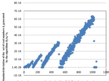
be noted that these uncertainties are associated with the concrete realization of operations (division and product) of numbers that generate the unit and as such, are not effectively the natural unit, but an approximation to the unity in real numbers. In order to visualize the behavior to which we are referring, in the following graph (Figure 1), we present the distribution of standard deviations of the first 1060 numbers generated by operations j i
i
b n
n ⋅ , with b
being a natural number, i ranging from 1 to 1000, and j ranging from 1 to 1060: As we can see in Figure 1, numerical uncertainty ai n
n
∆ ⋅
, with ai∧ ∈n N, generates p single sets of un- certainty with 2p points, with p∈N.
Potentiation introduces certain rules for small natural numbers, since until n = 100 we have that
1 n 1 n n n n n ∆ ⋅ ≅ ∆ ⋅ .
If n is a natural number and k the finite uncertainty of a real n generated by algebraic operations, we can find that ∆
( )
k =k or ∆( )
k =0 which means that the uncertainty produced by the same algebraic operations thatFigure 1. Relation between the standard deviation of the set of numbers that generate real numbers from 1 to 1060, using natural numbers from 1 to 1000.
acts on the uncertainty of the previous number n is the same or vanishes, that is: 1 1 1 1 n n n n n n ∆ ⋅ ⋅ = ∆ ⋅ ⋅
or
1 1 0 1 n n n n ∆ ⋅ ⋅ = ⋅ Obviously radicals can also produce numerical uncertainty, which means that 1 n k n
∆ ⋅ =
can be zero,
that is, ∆ k =0, or a multiple of k, or the result of a specific natural number multiplied by k. We have that 1 ( n) 0 n ∆ ∆ ⋅ =
, but on the contrary, we also have that:
2 1 1 ( n) n k n n ∆ ∆ ⋅ = ∆ ⋅ = . In general, a 1 n) 0 n ∆ ∆ ⋅ = and 1 1 ( ) a a n n k n n ∆ ∆ ⋅ = ∆ ⋅ =
, with a being a natural number.
If we focus on the expression 2 2
2 2 1 1 . 1 1 1 n n n n − ⋅ − ⋅
, and consider that 2 2
1
1 .n
n
− is not zero, we also find uncertainties for the real number one different from zero.
5. Numerical Uncertainty and Physics
The fine-structure constant α is a physical constant which characterizes the magnitude of electromagnetic force and was defined by the first time by Arnold Sommerfeld [4] as
2 0 2 e hc α ε
= , where e is the electron’s charge, ε0 the vacuum permittivity, h the Planck’s constant and c the speed of light in vacuum.
For some time now, physicists of the international scientific community have questioned themselves whether the so-called universal constants are actually “universal variants”, that is, capable of assuming new values as time goes by. If the fine-structure constant, even being an empirical constant, had a lower value, the density of atomic matter in the Universe would also be lower, with weaker connections under lower temperatures. If, on the contrary, the fine-structure constant were larger, the smaller atomic nuclei would not exist due to electric repulsion between protons. This interpretation of alpha can predict a physical outcome; even we do not assign it a real physical meaning. Others interpretations where proposed: α is the ratio of two energies or the ratio of the velocity of the electron in the Bohr model of the hydrogen atom to the speed of light, among others.
Richard Feynman, referred to the fine-structure constant in these terms:
“There is a most profound and beautiful question associated with the observed coupling constant, α - the am-plitude for a real electron to emit or absorb a real photon. It is a simple number that has been experimentally de-termined to be close to 0.08542455. (My physicist friends won’t recognize this number, because they like to re-member it as the inverse of its square: about 137.03597 with about an uncertainty of about 2 in the last decimal place. It has been a mystery ever since it was discovered more than fifty years ago, and all good theoretical phy-sicists put this number up on their wall and worry about it.) Immediately you would like to know where this number for a coupling comes from: is it related to π or perhaps to the base of natural logarithms? Nobody knows. It’s one of the greatest damn mysteries of physics: a magic number that comes to us with no understanding by man. You might say the “hand of God” wrote that number, and “we don't know how He pushed his pencil.” We know what kind of a dance to do experimentally to measure this number very accurately, but we don’t know what kind of dance to do on the computer to make this number come out, without putting it in secretly!” [5].
In fact, the numerical uncertainty Δ(0.08542455) is much lower than the numerical uncertainty of Δ(137.03597).The numerical error of 0.08542455 measured as the standard deviation of 1000 calculations of the type 0.08542455 n
n
has a value of 7.08393E
cal-culations of 2 1 0.08542455 n n
has a value of 2.50239E−12. Let us assume then that 137.03597 is the average
of the numbers generated in the previous operation and that if we take into account numerical uncertainty it will lead to an interval from137.03597 − 2.50239E−12 to 137.03597 + 2.50239E−12. In order to calculate the value of α mentioned by Feynman, for the number 137.03597 we have then two possibilities:
12 1 137.03597−2.50239 10× − and 12 1 137.03597+2.50239 10× −
which would generate the numbers 0.0854245499999992 and 0.0854245500000008 with standard deviations of 1.66398E−16and 1.40267E−15, re-spectively.
If the difference of 2 in the last decimal case related to the calculation of α, is connected to the calculation path, then it is possible that the two values are coincident with the numerical intervals obtained through their numerical uncertainty. In fact: (0.08542455 − 7.08393E−16) − (0.0854245500000008 − 1.40267E−15) = 0, which explains that the difference between the two values of the fine structure constant pointed out by Feynman may be due to the numerical uncertainty generated by the operations.
The fine-structure constant can also be calculated as 2 e
hR cm
α = [6]. We can equate both expressions for the determination of the fine-structure constant [5] and [6], and we reach:
2 4 2 2 2 0 0 2 2 2 e 4 e e hR e hR hc cm h c cm ε = ⇔ ε = ,
from where we obtain:
4 2 3
0
8
e
e m = ε h Rc (1) Since 8 h Rcε02 3 is the product of physical and mathematical constants, it must be constant, and so e m4 e
must be constant too, which means that there is an inverse relation between the electrical charge of the electron and their mass, except if the electron charge and the electron mass are not in rest, or the electron mass and charge are unchangeable at the atomic level, at least for low energy levels. For low energy levels the electron in the first Bohr orbit moves nears 1/137 of the speed of light.
From equation 1, is possible to compute the product e m4 e for an electron moving in different Bohr orbits, that means moving at speeds different from 1/137 of the light speed, where me will be the mass of the traveler electron with speed greater than the speed in the hydrogen atom. If this is possible what happens with the elec-tron charge in movement? Must this product be in all circumstances constant?
Recently Nair et al. [7] and Reed et al. [8] observed for graphene one amazing property. When light is shown through a large suspended membrane of graphite, most visible light passes right through it. However, graphene is not clear; about 2.3 percent of visible light is absorbed. Dividing this number by π gives the exact value of the fine structure constant, which is the fundamental physical constant that characterizes the strength of the electro-magnetic interaction. These results show that the movement of the electron is not restricted to the model of Bohr for the hydrogen atom.
Apparently, the reason why dividing the percentage of visible light shining through π gives the fine structure constant is that the electrons in graphene behave as if they have lost their mass. That could mean that the fine structure constant could physically represent more than a simple ratio between the speed of the hydrogen elec-tron and the speed of light in the vacuum.
Webb et al. [9] reported from the observations at the Keck telescope a smaller change in the value of the fine structure constant α at high red shift. The same authors suggest, with the data of the New Very Large Telescope (VLT), for a different direction in the Universe, that an inverse evolution occurs and α increases at high red shift. From here, it seems easier to explain the changes in the mass and charge of the electron than a change in the fine-structure constant, because no reason until know was found to explain changes in the vacuum permittivity, in the Planck’s constant, in the Rydberg constant or in the speed of light in the vacuum.
Nasseri [10] calculate the fine structure constant in the space time of a cosmic string. He shows that in the presence of a cosmic string the value of the fine structure constant reduces for a value of (1 − 8.736E−17)α, where α is known the fine-structure constant. This reduction is indeed very small.
When we calculate the numerical uncertainty for the fine-structure constant ∆
( )
α , as explained before, we found the value of 1.2236E−16 which is slightly larger than the calculated change of α from Nasseri [10] or the corrections made by Marques [11]. It will be difficult to explain changes in α due to an effect of a cosmic string, when the numerical uncertainty related to the algebraic operations are bigger than the calculated value of change, even we assume the adjustments proposed by Nasseri [12].Let us assume here an hypothetical physical relationship between the product
e
m
e4
and the product 2 3
0
8 h Rcε . If α changes it is due to a change in the velocity of the electron, or on their mass, as observed by Webb et al. [9]. Let us assume the electron as a free particle with a relativistic mass, in order to explain a possi-ble mass change of this particle.
If this is possible, Equation (1) shows that if the relativistic mass of the electron tends to infinity, due to a speed increase of the electron to light speed, its electrical charge would go down to zero. The idea that mass may reach infinity is also suggested by Einstein’s expression for the equivalence of mass-energy, which shows that the inertial mass of a particle varies with the relation 2
2 2 1 o m c E mc v c = = −
, where mo is the mass of a particle at
rest and m its mass when it moves at constant speed v.
However, if we allow either the mass or the electrical charge to reach infinity (where the other factor of the product e m4 e would become zero) such a product would result in a mathematical indetermination of the type
.
o∞, which means that either the mass of the electron does not tend to infinity when it moves at the speed of light, or the electric charge does not tend to zero when this material particle moves at speeds close to the speed of light, or, finally, that the product e m4 e, is not really constant, which means that there is a variation of the product of the physical and mathematical constants 8 h Rcε02 3 .
Any of the conditions exposed here generates paradoxical physical conditions, where the solution to the pa-radox may be in the fact that the fine-structure constant is calculated through different ways in order to obtain the same value, but there is no relation between the fundamental physical processes which underlie the calcula-tions, since we are merely dealing with algebraic relacalcula-tions, despite the two expressions having the same physical dimensions.
This issue raises problems in mathematics and philosophy which were present in the mind of scientists from Newton to Einstein, as noted above. Newton believed that Nature was continuous, and thus used geometry, ra-ther than algebra, since algebra provides only approximations which contain discontinuities. For Newton, only through geometry one can obtain a representation of nature where uncertainty is not introduced through alge-braic processes of approximation. Einstein uses Cartesian axes in his analysis without discussing its underlying presuppositions.
The introduction of algebra introduces numerical uncertainty which, if Newton is right, may introduce uncer-tainty and discontinuity where it does not exist. Or it may be the case that Newton was wrong and Nature is dis-continuous. In that case, algebra, rather than geometry (numbers, rather than figures), capture an aspect of reality, rather than introducing uncertainty into a certain reality. Whatever is the case, we can certainly benefit from a study of the nature of the instrument we are using when studying Nature and the Universe, in order to infer the extent to which we are capturing an aspect of reality, or imposing our framework into reality.
When we admit speeds of the electron greater than the velocity of the electron in the hydrogen atom, a loss of mass of the electron (has observed by Nair et al. [7] and Reed et al. [8]) leads to a sort of charge excess, either locally or globally, or alternatively resorts to the continual creation of ions.
Davies [13] when trying to explain the time dependence of the fine structure constant argued that the only way to explain theoretically the change in the fine structure constant is by postulating some form of charge excess, for instance as an inequality in electron and proton numbers, or a polarization due to electric fields “frozen in” to the cosmological metric. In condensed matter physics the existence of quasi electrons with numerical and ana-lytical fractional charge is admitted. Quasi particles are emergent phenomena that occur when a microscopically complicated system such as a solid behaves as if it contained different weakly interacting particles in free space. With these issues in mind, let us explore the uncertainty associated to the algebraic expression of Equation (1). The physical and experimental uncertainty when calculating the c, ε0, h and e constants is frequently changing due to improvement of the accuracy of laboratory processes. These physical constants can take many dimen-sional forms, such as the case of the speed of light, or be dimensionless, as the fine structure constant α.
mass or charge of the electron. If we admit that Equation (1) has a physical meaning, we are then led to believe in the existence of an inverse connection between mass and charge as reached above.
Now, in Millikan’s experiences, the measurement of the electrical charge of the electron is determined through variables which depend upon the electron’s mass [14]. If we look at the determination of mass and charge of the electron by the International Council for Science: Committee on Data for Science and Technology [15], we are again led to the conclusion that it is impossible to determine simultaneously the charge and mass of the electron, and this happens both for low speeds or for high speeds.
If we admit a relativist change in the electron’s mass, through Equation (1), we are led to the conclusion that there is also a relativistic variation in the electron’s charge, which should lead, through the product e m4 e, to the exact value 8 h Rcε02 3 , or an approximate value given by their numerical uncertainty. Under those circumstances, we find that for calculations made with values of the electron speed up to 99.999% of the speed of light, numer-ical uncertainty of the product above is:
(
4)
121(
4)
7.7452 C .kg
e
e m E−
∆ ≥ or ∆
(
e m4 e) (
=0 C .kg4)
(2) where me is again relativistic.Figure 2 shows the variation of the product e m4 e when the electron’s speed reaches a value very close to the value of the speed of light in the vacuum, where the electron’s charge was allowed to vary together with the electron’s mass, so that the product e m4 e would remain constant:
This shows that positive numerical uncertainty associated with e m4 e has no relation with the speed of the particle, and appears to have a random distribution with values between zero and near 9E−120 C4 kg. Numerical uncertainty is here the absolute value of the difference between e m4 efor a given speed, and the value we would obtain through the relationship with 8 h Rcε02 3 . So far, we have no reason to postulate that uncertainty corres-ponds to an underlying physical process. Rather, it can be taken to be the result of algebraic approximations.
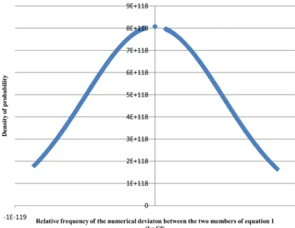
It is assumed that the two members of Equation (1) are equal, term by term, with the same nil result, except if we use approximations. A study of numerical uncertainty, measured as the difference between the two members of equation 1, shows that its statistical distribution is Gaussian, with a mean of −7.6687E−122 C4
kg and a stan-dard deviation of 4.9359E−120 C4 kg. That means, for example, that a percent error of measurement of the elec-tron’s charge of 8.71E−33 C, increases the numerical uncertainty by a factor of 10.3, which is still very small when compared to experimental uncertainty.
Figure 3 shows the distribution of numerical uncertainty of the difference between e m4 e and 8 h Rcε02 3 . The most likely value of the difference between e m4 e and 8 h Rcε02 3 is a value close to zero with a proba- bility of occurrence of 0.089, in an interval or ratio v
c between 0.01% and 99.99%. The difference between
Figure 2. Variation of absolute deviation or numerical uncertainty between the two members of the equation 1 when the electron’s speed approaches the speed of light in the vacuum.
Figure 3. Statistical distribution of the numerical uncertainty of the difference between 4 e e m and 2 3 0 8ε h Rc 4 e
e m and 8 h Rcε02 3 is near zero when
1000
nc
v= (3) where n is part of N, but n assumes only specific values of N. The rule of the values assumed by n is connected to the numerical uncertainty produced.
6. Relations between Speed, Mass and Charge
If Equation (1) is physically valid, then there is no reason to believe that Equations (2) and (3) are not valid too. Thus, the electron may well be above the speed of light in the vacuum, even if the uncertainty surrounding e m4 e does not increase greatly, or if v
c cannot assume values above 99.99% c, which may generate no uncertainty.
Once again we have, essentially by Equation (3), quantic numerical uncertainties, as was observed early in the expressions of the numerical approximation and calculus path dependence.
A numerical uncertainty of this type, for values above the speed of light, only results in a basic randomness in the electron’s movement, as a particle electrically charged, and a limited statistical predictability of the behavior of this apparently quantic system.
We can see the variation between n’s (from Equation (3)) which lead to almost zero uncertainty as n increase, and independent of the speed of the electron. It is easy to see that there is not a clear tendency, but as speed in- creases, the behavior appears to be similar to that of uncertainty of the type 1 n
an
∆ ⋅
, which can be expressed
as 2n 1n 2nk
n
− ∆ = −
, where we need to determine k if we want to identify a similarity, for the constant α, that
is not a natural number in this case, but a finite real number to be determined and also subject to numerical un-certainty. If we look carefully for this property there is a slight decrease of uncertainty as speed increases.
By the Equation (3), apparently, there is no convergence (or a tendency for nil uncertainty) to zero as the speed of the electron approaches the speed of light. If there is any such convergence, it exists only for values above the speed of light.
If convergence is of the type 1 n an
∆ ⋅
, then we must divide the fourth power of the electron’s charge by a
the numerical uncertainty of e m4 e is zero for values above the speed of light in the vacuum, then we are in a case where we cannot find algebraically the zero value or the infinity in one of the factors of the product e m4 e.
Einstein’s equation restricts the electron’s movement to a speed below the speed of light in the vacuum, which would mean that the behavior observed above has no physical meaning, but Bertozzi’s [16] study suggests that electron’s have been accelerated up to a value close to the speed of light, using potential energy greater or equal than 15 MeV, without their mass becoming infinite. Livingston and Blewett [17] show that in specific conditions the mass of a moving electron is equal to its rest mass, and the speed of light can be reached without the mass becoming infinite.
Thus, if Equation (1) would have physical meaning the mass of the electron, as its charge, would be relativistic variants. This does not challenge Einstein’s relativity theory. It only means that the speed of light in the vacuum may not be the highest existent speed in the Universe because the electron may travel at a faster speed, due to its physical mass singularity.
We can measure the speed of an electrically charged particle through Cherenkov’s radiation, or Cherenkov’s effect [18], where speeds above light in a medium are reached. Saltzberg et al. [19] studied a similar effect, the Askaryan’s effect, where a particle travels above the speed of light in a medium than the vacuum. Askaryan [20] had also seen an excess of negative electrical charge, absorbed by matter or removed by the photo-electrical effect, or through positron-electron interactions. Saltzberg et al. [19], Gorham et al. [21] and Gorham et al. [22] also saw similar effects in different mediums.
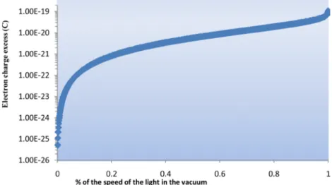
These experiments suggest an interaction between electrical charge (which may exist in excess) and the speed of the particle. If the mass and charge of the electron change with its speed, when the electron passes from vacuum to other environments at a high speed, its speed will diminish, and the observed physical effect will be an apparent loss of electrical charge.
Figure 4 shows the range of variation of the expected excess of electrical charge if an electron travelling close to the speed of light in the vacuum and reach to a different environment, losing speed as change of medium consequence.
We have no algebraically or physical reasons for denying the possibility that Equation (1) reflects a physical relationship, which seems to translate a clear dependence between the electron’s mass and charge, leading to the appearance of another level of uncertainty, connected to the simultaneous determination of their mass and charge.
7. Concluding Remarks
Whitehead [23] formulated a theory of relativity, which received little attention comparatively to Einstein’s. There is, however, one aspect at least that was developed by Whitehead to a greater extent than Einstein, deserving closer attention. This aspect is the philosophical implication that science has for our conception of reality. Whitehead [24] was later led to concluding that reality constitutes a process, as Heraclitus argued long ago. The fact that the electron’s charge and mass might change with its speed is another instance of this philosophical as-pect. Free electrons, as a part of reality, are a process which is permanently changing, and probably its speed, mass and charge, cannot be taken to be always fixed.
The fact that reality is a continuous flow, raises the question of how to grasp knowledge of a reality which is permanently changing, where it is not only the speed of a particle, but also its mass and charge, which are changing. Plato’s solution, which was also followed by Whitehead and was already adopted before by the Pythagorean school, is to grasp the forms (geometrical figures and natural numbers) that reality assumes in this permanent flow. We can identify equations, like Equation (1), which give us some knowledge of the process of change and try to reach conclusions based on mathematical operations.
Mathematical operations are, however, subject to uncertainty, which must be taken into account when using mathematics. Whitehead and Russell [25] tried to provide exact foundations for mathematics. Gödel’s incom-pleteness theorem undermined this prospect. Since Pythagoras and Plato, there has been a belief that reality possesses a mathematical structure to be discovered. Even Newton, who was aware of the fact that algebraic processes provide only approximations, still believed that a proper geometrical method (freed from algebra) could provide an exact description of reality, which Newton believed was continuous, rather than discontinuous.
For example, the Lorentz transformations can be described using the geometrical method that Newton used in his Principia, as the variation (the derivative) of the arc of a sinusoidal function of v
c. This would eliminate
numerical uncertainty by using a geometrical method instead of an algebraic method, following Newton’s phi-losophy, according to which Nature should be described in geometrical terms, rather than through algebraic processes that contain uncertainty because they only provide approximations.
These philosophical considerations are not an additional curiosity, but an essential ingredient for the devel-opment of mathematics and science. The results discussed above, concerning the relation between speed, mass and charge of particles, can only be properly addressed within a wider field, which encompasses those considerations. Amongst the discussions to take place, a central one is whether the reality we are studying is best seen in terms of processes or particles, as a continuous or a discontinuous entity.
REFERENCES
[1] M. Atiyah, “Collected Works,” Oxford University Press, Oxford, 2005.[2] N. Guicciardini, “Isaac Newton on Mathematical Certainty and Method,” MIT Press, Cambridge, 2009. [3] A. Einstein, “The Meaning of Relativity,” Princeton University Press, Princeton, 1922.
http://dx.doi.org/10.4324/9780203449530
[4] M. Eckert, “Arnold Sommerfeld: Science, Life and Turbulent Times, 1868-1951,” Springer, New York, 2013.
http://dx.doi.org/10.1007/978-1-4614-7461-6
[5] R. P. Feynman, “QED: The Strange Theory of Light and Matter,” Princeton University Press, Princeton, 1985.
[6] G. Gabrielse, D. Hanneke, T. Kinoshita, M. Nio and B. Odom, “New Determination of the Fine Structure Constant from the Electron g Value and QED,” Physical Review Letters, Vol. 97, No. 3, 2006, Article ID: 030802.
[7] R. Nair, P. Blake, A. Grigorenko, K. Novoselov, T. Booth, T. Stauber, N. Peres and A. Geim, “Fine Structure Constant Defines Visual Transparency of Graphene,” Science, Vol. 320, No. 5881, 2006, p. 1308.
[8] J. Reed, B. Uchoa, Y. Joe, Y. Gan, D. Casa, E. Fradkin and P. Abbamonte, “The Effective Fine-Structure Constant of Free-standing Graphene Measured in Graphite,” Science, Vol. 330, No. 6605, 2010, pp. 805-808.
http://dx.doi.org/10.1126/science.1190920
[9] J. K. Webb, J. A. King, M. T. Murphy, V. V. Flambaum, R. F. Carswell and M. B. Bainbridge, “Indications of a Spatial Varia-tion of the Fine Structure Constant,” Physical Review Letters, Vol. 107, No. 19, 2011, Article ID: 19110.
[10] F. Nasseri, “Corrections to the Fine Structure Constant in D-Dimensional Space from the Generalized Uncertainty Principle,”
Physical Letters B, Vol. 618, No. 1-4, 2005, pp. 229-232.http://dx.doi.org/10.1016/j.physletb.2005.05.050
[11] G. Marques, “Comment to: ‘Corrections to the Fine Structure Constant in the Spacetime of a Cosmic String from the General-ized Uncertainty Principle’,” Physical Letters B, Vol. 638, No. 5-6, 2006, pp. 552-553.
http://dx.doi.org/10.1016/j.physletb.2006.06.012
[12] F. Nasseri, “Reply to: ‘Comment to: Corrections to the Fine Structure Constant in the Spacetime of a Cosmic String from the Generalized Uncertainty Principle’,” Physical Letters B, Vol. 645, No. 5-6, 2007, pp. 470-471.
http://dx.doi.org/10.1016/j.physletb.2006.12.033
[13] P. Davies, “Is the Universe Transparent or Opaque?” Journal of Physics A: General Physics, Vol. 5, No. 12, 1972, pp. 1722- 1737.http://dx.doi.org/10.1088/0305-4470/5/12/012
3, 1995, pp. 197-214.http://dx.doi.org/10.1007/BF02628797
[15] P. Mohr, T. Barry and D. Newell, “CODATA Recommended Values of the Fundamental Physical Constants: 2010,” Reviews
of Modern Physics, Vol. 84, No. 4, 2012, pp. 1527-1605.http://dx.doi.org/10.1103/RevModPhys.84.1527
[16] W. Bertozzi, “Speed and Kinetic Energy of Relativistic Electrons,” American Journal of Physics, Vol. 32, No. 7, 1964, pp. 551-555.http://dx.doi.org/10.1119/1.1970770
[17] S. Livingston and P. Blewett, “Particle Accelerators,” Mcgraw Hill Book Co. Inc., New York, 1962.
[18] D. Landau, M. Liftshitz and P. Pitaevskii, “Electrodynamics of Continuous Media,” Pergamon Press, New York, 1984. [19] D. Saltzberg, P. Gorham, D. Walz, C. Field, R. Iverson, A. Odian, G. Resch, P. Schoessow and D. Williams, “Observation of
the Askaryan Effect: Coherent Microwave Cherenkov Emission from Charge Asymmetry in High Energy Particle Cascades,”
Physical Review Letters, Vol. 86, No. 13, 2001, pp. 2802-2805.http://dx.doi.org/10.1103/PhysRevLett.86.2802
[20] G. Askaryan, “Excess Negative Charge of an Electron-Photon Shower and Its Coherent Radio Emission,” Soviet Physics
JETP-USSR, Vol. 14, No. 2, 1962, pp. 441-443.
[21] P. Gorham, D. Saltzberg, R. Field, E. Guillian, R. Milincic, D. Walz and D. Williams, “Accelerator Measurements of the Askaryan effect in Rock Salt: A Roadmap Toward Teraton Underground Neutrino Detectors,” Physical Review, Vol. D72, 2005, 16 p.
[22] P. Gorham, S. Barwick, J. Beatty, D. Besson, W. Binns, C. Chen, P. Chen, J. Clem, A. Connolly, P. Dowkontt, M. DuVernois, R. Field, D. Goldstein, A. Goodhue, C. Hast, C. Hebert, S. Hoover, M. Israel, J. Kowalski, J. Learned, K. Liewer, J. Link, E. Lusczek, S. Matsuno, B. Mercurio, C. Miki, P. Miocinovic, J. Nam, C. Naudet, J. Ng, R. Nichol, K. Palladino, K. Reil, A. Ro-mero-Wolf, M. Rosen, D. Saltzberg, D. Seckel, G. Varner, D. Walz and F. Wu, “Observations of the Askaryan Effect in Ice,”
Physical Review Letters, Vol. 99, No. 17, 2007, 4 p.
[23] A. N. Whitehead, “The Principle of Relativity,” Cambridge University Press, Cambridge, 1922. [24] A. N. Whitehead, “Process and Reality: An Essay on Cosmology, Macmillan, London, 1929.