1
The
re
la
t
ionsh
ip
be
tween
rea
l
es
ta
te
and
econom
ic
cyc
les
:
ev
idence
from
the
USA
Author: João Mendes
Dissertation written underthe supervision of Joni Kokkonen
Dissertation submittedin partial fulfillment of requirements forthe MSc in Finance, atthe Universidade Católica Portuguesa, July 2017
3 Abstract
This study challenges the possibility of defining a strategy to invest in the real estate area, avoiding incurring in bubbles or crises. Mainly based on REITs approach as an investment proxy, it covers the study of several periods in the last three decades through an economic and statistical view, in order to deepen the investigation on real estate and economy relationship. In addition to find that REITs quarterly yield is around 1.05% with a standard deviation around 11.10%, the study reveals that during half of the considered time these funds may return four times that amount. It becomes crucial then to identify those moments, in a medium to long-term strategy, therefore, using the economic cycle as the explanatory variable. Through a system of regressions with R’s-squared within [0.87;0.95], we concluded the best variables to successfully conduct this model are the GDP, the 3-month Treasury interest rate, the unemployment rate and the consumer confidence index, being consistently significant, whereas industrial production and real estate indices do not fit in this method. Surprisingly, unemployment may contribute positively to real estate returns in this scenario, and the most unstable variable is the GDP as it may weigh more than the predicted.
Resumo
Este estudo desafia a possibilidade de definir uma estratégia de investimento na área do imobiliário, evitando bolhas especulativas e crises. Principalmente baseado numa perspetiva que utiliza o tipo de fundos REITs como intermediário de investimento, o estudo lança um olhar para vários períodos nas últimas três décadas através duma visão económica e estatística, de forma a aprofundar a investigação da relação entre o imobiliário e a economia. Para além de mostrar que os REITs trimestralmente oferecem retornos na ordem dos 1.05%, com um desvio-padrão de 11.10%, o estudo revela que, durante metade do tempo em análise, estes poderiam obter retornos quatro vezes maiores que esse montante. Torna-se crucial identificar esses momentos, numa estratégia de médio a longo prazo, e por essa razão, utilizando o ciclo económico como variável explicativa. Através dum sistema de equações de regressão com coeficientes de determinação no intervalo [0.87;0,95], concluímos que as melhores variáveis a utilizar são o PIB, a taxa de juro do tesouro a 3 meses, a taxa de desemprego e o índice de confiança do consumidor, sendo consistentemente significativos, enquanto que os índices de produção industrial e imobiliário não se enquadram convenientemente no modelo. Surpreendentemente, o desemprego pode contribuir positivamente nos retornos do imobiliário neste cenário, e a variável mais instável é o PIB, uma vez que poderá ter um peso maior do que o previsto.
4 Acknowledgments
First of all, I would like to thank Universidade Católica for the opportunity of joining one of their well-known masters of science, as it was and it is a great opportunity for any student who looks forward to entering the labor market, especially in the financial and management areas. I could tremendously improve my analytical and judging skills, work with new research and statistical software, but most importantly, make new friendships either with colleagues or professors. Without the resourceful hand from this institution, I would not have reached this stage in my life, and aspire to reach future high goals in my professional life.
Secondly, I want to thank my advisor in this process, the professor Joni Kokkonen, whose knowledge in financial and investment areas knows no limits. Among the several seminars offered to do the thesis project, I opted for the one which was lectured by Joni, not only because it was the one which caught my attention the most, but also because I enjoyed very much the previous course lectured by him. He was always available to give his advice and clarify so many questions that arose during this project, that in the end it was not possible to do it only by myself.
Last but not least, I have to thank my family and friends, since all of them without exception contributed with ideas when I was asked about my theme. Specifically, I want to thank my girlfriend Mariana Pereira da Silva for her support and care during the long hours she stayed by my side and my best friend Francisco Nuno Lopes, for his interest in all my accomplishments. Both were always bringing ideas to the table and together started endless discussions which highly contributed to do my thesis.
5 I Contents List
I Contents List ... 5
II List of Figures and Tables ... 6
III List of Abbreviations ... 8
1. Introduction ... 9
2. Literature Review ... 12
3. Data ... 15
3.1 Data definition ... 15
3.2 Data gathering ... 15
3.3 Data statistics and correlation ... 18
4. Methodology ... 22
4.1 Choosing the best model ... 22
4.1.1 Real estate index ... 23
4.1.2 REITs returns... 24
4.1.3 REITs NAV ... 25
4.2 Testing the model ... 28
4.2.1 Scenarios analysis ... 28
4.2.2 Enlarging sample ... 31
4.3 Identifying the ideal periods ... 32
5. Conclusions ... 37
6. Appendices ... 38
6 II List of Figures and Tables
Graph 1. Number of households in the USA. ... 9
Graph 2. Real estate sector in the USA (% of GDP). ... 10
Graph 3. GDP cycle after HP filter (quarterly, λ = 1600). ... 33
Graph 4. 3-month Treasury bill rate after HP filter (quarterly, λ = 1600). ... 34
Graph 5. Unemployment rate after HP filter (quarterly, λ = 1600). ... 34
Graph 6. Consumer confidence index after HP filter (quarterly, λ = 1600). ... 35
Graph 7. 3-month Treasury bill rate since 1970. ... 38
Graph 8. Unemployment rate after HP filter since 1970 (quarterly, λ = 1600).. ... 38
Table 1. Thesis guiding questions. ... 10
Table 2. Database filters ... 16
Table 3. Variables specifications. ... 18
Table 4. Variables statistics. ... 19
Table 5. Economic variables correlations ... 20
Table 6. 9 REITS group and REI correlations table. ... 21
Table 7. Real estate index regression. ... 23
Table 8. REITs returns regression. ... 25
Table 9. Equation 4 coefficients and corresponding significance ... 27
Table 10. Equation 5 coefficients and corresponding significance. ... 28
Table 11. Scenarios with changes and REITs output. ... 29
Table 12. Statistical measures from changes in explanatory variables ... 30
Table 13. Coefficients comparison of different samples. ... 31
Table 14. Aggregated periods, returns and residuals. ... 32
Table 15. Official definitions of sectors and investment instruments. ... 39
Table 16. 9 funds selection analysis ... 40
Table 17. Regression output CGMRX.O. ... 42
Table 18. Regression output CSRSX.O. ... 42
Table 19. Regression output DFREX.O. ... 43
Table 20. Regression output EGLRX.O. ... 43
Table 21. Regression output FREEX.O. ... 44
7
Table 23. Regression output PWREX.O. ... 45
Table 24. Regression output RPFRX.O. ... 45
Table 25. Regression output STMDX.O. ... 46
Table 26. Regression output CGMRX.O. ... 46
Table 27. Regression output CSRSX.O. ... 47
Table 28. Regression output DFREX.O. ... 47
Table 29. Regression output EGLRX.O. ... 48
Table 30. Regression output FREEX.O. ... 48
Table 31. Regression output FRESX.O. ... 49
Table 32. Regression output PWREX.O. ... 49
Table 33. Regression output RPFRX.O. ... 50
8 III List of abbreviations
BLUE – Best Linear Unbiased Estimators
CMBS – Commercial Mortgage-Backed Securities CPI – Consumer Price Index
CV – Coefficient of Variation FCF – Free Cash-Flow
GDP – Gross Domestic Product HPR – Holding Period Return HP – Hodrick-Prescott
IPO – Initial Public Offer LM – Lagrange Multiplier
MUIT – Mutual fund and Unit Investment Trust NAHB – National Association of Home Builders
NAICS – North American Industry Classification System NAV – Net Asset Value
OLS – Ordinary Least Squares RE – Real Estate
REI – Real Estate Index
REIT – Real Estate Investment Trust
SEC – Securities and Exchange Commission USA – United States of America
9 1. Introduction
Real estate is a vast area in every country, since it always is a considerable slice of their GDP, as well as of their economy. We are constantly observing cities growing and developing, through their expansions to suburb areas or in more recent decades in height, like skyscrapers. Besides, not only people’s apartments and houses are part of the real estate sector, since it is a wide sector that includes both residential services and instruments for personal or corporate investment. As it can be seen in the graphs below, the real state is a big sector in the USA. With approximately 325 million people, the USA also has quite a big number of houses (134.7 million), a bit less than half of its population, and taking into account the last 30 years, it will continue to grow (graph 1). In addition, it has always had a major slice of its GDP exclusively coming from the real estate. According to graph 2, the total investment since 1985 in that area has always been almost 20%, which means that followed the growth in GDP, with the distinction between residential services and residential fixed investments. Following our definition of real estate, we conclude that this GDP percentage is spent in all the establishments engaged in renting or leasing real estate as well as managing selling, buying, renting or providing real estate services for others.
Graph 1. Number of households in the USA. Data from the bureau of census.
- 20 40 60 80 100 120 140 160 1985 1990 1995 2000 2005 2010 2015 Millio ns Year Total Households Occupied households
10 Graph 2. Real estate sector in the USA (% of GDP). Data from NAHB.
Being aware of real estate potential because of its dimension, we want to deeply investigate the question about its relationship with the economic cycle. First of all, we should define our strategy based on guidelines as it will be discussed in the next paragraphs.
The main objective of this investigation can be written as it follows:
1. Explain the relationship between economy and real estate using REITs historical performance since 1995 in order to identify returns’ increases or decreases justified by the economic cycle through an econometrical model. To the main objective we add a few more questions which will be taken into consideration during our investigation, with more specific features:
1. Explore and decide about macroeconomic variables that fit our econometric analysis the most.
2. Test the model at several levels in order to check its consistency and identify the ideal periods.
With these questions, we prepare an econometrical model based on the following table, so that our variables and goals are disposed and organized:
0% 2% 4% 6% 8% 10% 12% 14% 16% 18% 20% 1985 1990 1995 2000 2005 2010 2015 Per ce ntag e of GDP Year Residential Fixed Investments Residential services Total
11 Table 1. Thesis guiding questions.
To investigate Questions/Hypotheses Variables to study Economic cycle
different approaches;
Which is the best method to model the economic cycle?
GDP, Consumer Confidence, Industrial Production, Unemployment, Treasury Bill,
RE Index The relationship
between economic cycle and real estate
returns;
Do real estate variables fit in the econometric model? What is the
relationship?
REITs, RE Index
Potential scenarios to apply the model.
Will the model remain consistent after adjusting the sample or the
time frame?
Sample size, time frame
After establishing the guidelines, we will discuss about what has already been studied, what further discoveries would be interesting and mainly an overview of real estate today’s conditions. There are several types of investment in this area, and around them different comprehensions, outcomes and bureaucratic rules. Therefore, we try to analyze the general picture so that our work eventually becomes more specified and accurate. Furthermore, we present the data and methodology used and the reasoning behind it. We mainly focus our approach on REITs, and explain how the research was conducted and filtered. Then, a series of regressions take place, with two different time-series samples, in order to improve the first results and until achieving a good level of consistency. In the end, it is important to check for the methodology feasibility to identify the best periods of returns in this area.
In general, we observed the advantages of using GDP, interest rate, unemployment rate and consumer confidence index in our model, dropping the industrial production index and the real estate index in both sides of the equation, which resulted in a more consistent model. In the end, we find how to take advantage of about half the time considered, resulting in superior returns rate. During these halves, the returns level was four times bigger than the whole period quarterly return rate of 1.05%.
12 2. Literature Review
2.1 Modelling and forecasting economic cycle
The first thing to question is what variables are more suited to explain the economic cycle, despite the large amount of literature about it.
Leamer (2001) shows the relationship (among other variables) between US cycle and economic variables like GDP, unemployment and interest rates. In his research it is mainly used the growth of real GDP to identify the cycles: the six economic expansions analyzed using GDP growth were concluded to have 14, 35, 10, 20, 31 and 39 quarters, which represents a high level of unpredictability. Afterwards, regarding the expansion periods, and despite missing the last twenty years in his research, there is already great evidence of the relationship with unemployment. In his work, it is shown that although it remains low most of the expansion period, the relationship is not completely linear, as unemployment may keep rising during the first quarters of an expansion. Then, the unemployment rate quickly decreases during recovery periods to its normal levels, attributable to its cyclic characteristic. Another considered variable is the 3-month Treasury bill rate, whose relationship with the cycle was considered through the difference between the 10-year Treasury bill rate and itself, reflecting high intermediation margins to banks when it is higher, but less profitable when it is lower. This difference is the “... measure that best tracks the life cycle of an expansion”. However, as it is referred, the Federal Reserve Board is able to change more easily the short-term rate than the long-short-term one, making it more predictable and of future analysis interest. Indeed, (see in the appendices section, graph 7) there was a moment in history with unexpected sharp increases and falls (in 1980, reaching to a monthly maximum of 15.66% and a minimum of 7.00% in the same year), due to some coincidences (Homer & Sylla, 1996, pp. 366-385): inflation was rising and the Federal Reserve tried to maintain interest rates at high levels; “an atmosphere of crisis pervaded the markets both in the United States and abroad” which led to a change in monetary policy by letting interest rates meet their balance through freely crossing supply and demand, resulting in “unprecedented volatility of rates and yields, and their climbing in late 1981 to the highest levels in the US history.”
To conclude, there are several obstacles to overcome when trying to forecast any of these cyclic variables, mainly because of their destabilized/non-linear trends (except for GDP, which slowly grows over time in the USA), as well as the different cycles duration, (although
13 unemployment cycle component is more less predictable within ranges from 5 to 7 years)1, and even because of unexpected situations like the monetary policy change in the 1980 which led to the early 80’s recession.
Other studies related to economic cycles predictability by several different variables were conducted, more relevantly the consumer confidence, and although it was not found significant forecasting ability in most of the years analyzed, it “... would have been helpful in predicting the 1991 recession.” (Batchelor & Dua, 1998). Furthermore, there was also evidence that its ability gets stronger if falls sustain longer. That may be due to the existing correlation as explained by (Blanchard, 1993), even if “... consumption shocks are simply followed by the changes in income which triggered them in the first place; consumption shocks are a mirror, not a cause” of falls in economy.
2.2 Relationship between economic cycle and real estate
From times to times, there is a growing belief that real estate market is a very trustworthy and spectacular area to invest, mainly in the long-term, as if the house prices could only increase. This “animal spirit” as treated by Akerlof and Shiller (2009, pp. 149-157) in the chapter “why do real estate markets go through cycles”, is responsible for bubbles. These bubbles are unconditionally linked to the economic cycle, either sometimes as a cause or more usually as a consequence, and Bates, Giaccotto and Santerre (2014) tested the cointegration using Johansen cointegration test and investigated it by distinguish housing market (which includes the services related to renting) from real estate economy while testing it. Overall, global economy has a stronger effect on real estate economy than considering only the house price and the housing market, mainly in the short-run. This is a good indicator to use REITs instead of house price, since they reflect the whole real estate economy as well as exclusively in the investor point of view.
Concerning investment products, older studies like Mueller and Ziering (1992) sought for the best diversifying strategy using holding period returns and standard deviations, considering both regional (by regions) and economical (employment related) ones. They found that taking into consideration employment resulted in a superior real estate portfolio diversification strategy than geographic diversification which suggests that higher correlations between economy and real estate exist. More specifically about REITs, Sagalyn’s (1990)
1 Starting in 1969, 1974, 1979, 1984, 1990, 1995, 2001, 2007, 2014, describing a right skewed shaped pattern during that time (see in the appendices section, graph 8).
14 already looked at these investment vehicles, explaining their composition and their behaviour with the economic cycle in terms of excess returns and risk (volatility), proving they most likely work like “publicly traded stocks” since the returns are securitized. At the same time, they are still different and as concluded by Lee and Stevenson (2007), will add diversification value to a portfolio of stocks.
More recently, some studies rejected a few ideas about their relationship in the financial markets, like being more speculatively traded and resulting in worse future performances, despite the speculation increase in times of economic boom, showing a strong correlation with economic cycle (Blau & Whitby, 2014). For this reason (among others), one of the study’s conclusions is that REITs do not badly affect the markets in terms of quality. In the same way, the traditional idea that institutional investors tend to invest passively and avoid short-term positions over long-term ones is rejected in the analysis of Devos, Ong, Spieler and Tsang (2013), since results indicated a reversal situation in times of economic change and they concluded that “... institutional ownership increased prior to the financial crisis, declined significantly during the period of market stress, but rebounded after.” Moreover, this matches the idea exposed by Zhou and Anderson (2013) of herding behaviour “under turbulent market conditions”, and in that specific case, “extremely turbulent”, leading to the conclusion that during some economic phases of the cycle like falls or sharp falls, unexpected behavioural components start having strong influence. Another example of this is the high volume in the CMBS market because of hedging rush (mainly) from financial institutions during the financial crisis 2007-2009, leading to mispricing, even if temporarily (Driessen & Hemert, 2012).
Despite all literature about crises behaviours in turn of real estate investment, not much has been studied in order to specifically aim to certain moments of cycles to filter returns, however, there are some practical studies which find the best strategies in the real estate sector. Amédée-Manesme, Barthélémy and Prigent (2015) investigated the best portfolio strategy, using the FCF and the terminal value, where variables like real estate market volatility and risk aversion level are considered to compute the optimal time to sell and the loss for not selling in the best time. Among several conclusions, they found within their model it is better to wait more before selling if the risk aversion is lower (the opposite also holds) and that when volatility increases it is better to sell faster, although it is also “negligible”.
15 3. Data
3.1 Data definition
It is important to understand the reason behind choosing REITs, and the first thing to analyze is their definition, which is their function in the economy. We opted to work with open-end investment funds, and according to the NAICS, these are legal entities which work as organized assets pools consisted of securities and other financial instruments. They are initially sold in IPOs, and then the shares transaction processes continue like in common companies, with the share price being settled by the NAV (see in the appendices section, table 15). There are some differences among REITs, since they can vary according to their nature (healthcare related investments in hospitals and similar buildings, economical related investments in enterprising buildings or shops and businesses, mortgage related which are based on debt instead of assets), although for our analysis it will not be important to distinguish them, since we want to prove the relationship of investing in real estate as a whole. But since we included all types, there is another classification to mortgage REITs as they are part of a different industry, which is related to debt holding instead of assets, with slightly different legislation but still in the real state sector (see in the appendices section, table 15).
3.2 Data gathering
Since REITs are somewhat recent financial instruments, we divide our research in two parts: one with longer time span and macroeconomic variables, whose data are very accessible, making it possible to relate with a real estate index and understand economically the relationship with the real state sector for a longer period; another with shorter time span, but based only on REITs, since data are available in these last years, and they stand as a great investment vehicle for real estate sector.
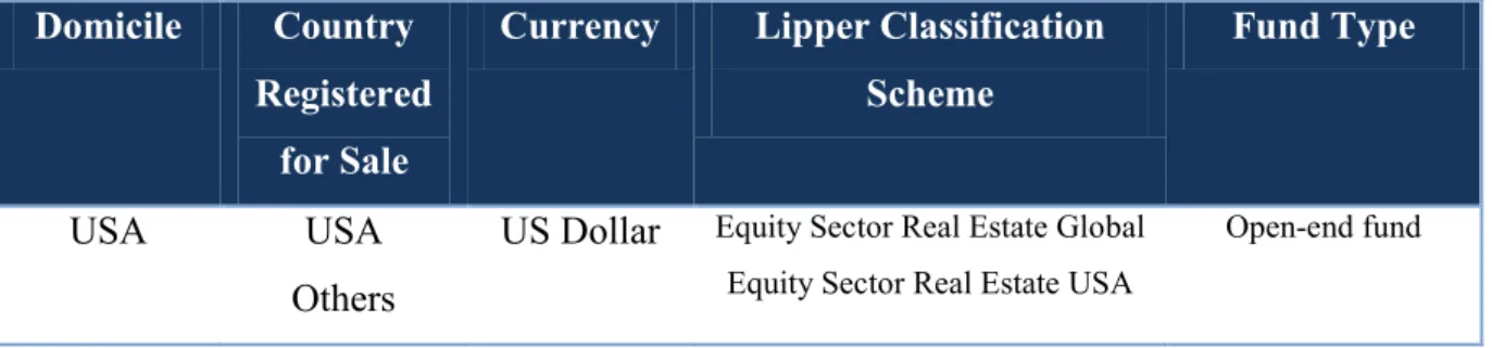
In order to obtain REITs data, we opt to use Thomson Reuters Eikon Terminals because of its wide access to instruments and indicators. We also prefer to analyze the US reality for logistic reasons as it reflects a cleaner overview as well as it is possible to obtain more data with higher time ranges. We selected our sample based on the criteria of table 2. It is important to note that although all funds have their domicile in the USA (the place where business is implanted), they may be also registered in other countries for sale, like Chile. In
16 addition, some of the funds’ assets come from other countries, giving the fund a classification of equity sector real estate global. The reason behind not filtering strictly to US real estate is to widen the variety of funds, knowing that the US economy is quite open to the world as well as its economical variables and investments in real estate.
Table 2. Database filters.
After applying the filters above, we were able to extract about 450 funds under these circumstances starting in different dates (from 1989 onwards), although we had to remove some because using NAV per share was not possible, either because they were lacking the daily quotation or missing big periods of information. Because of this impossibility, we closed our sample with 413 funds. This sample composed of REITs was done in order to quarterly return both its NAV per share and average of daily returns, which were calculated by the following formula:
( 1 ) where i represents each day when it was negotiated. Then, we computed the sum of every daily return in each month, and later on in each quarter. In addition, we decided to compute it in a way that all funds have their own different initial dates and negotiation dates (which may occasionally be different due to extraordinary factors like closing the negotiation in a specific day for that fund). This gives different possibilities to set the initial period of our sample, and include either a bigger or smaller number of funds. Besides, dividing the analysis by quarters allows us to compare and use all funds together, even if some of them had a different number of days in some months. The analyses will target a group of 9 REITs (see in
Domicile Country Registered
for Sale
Currency Lipper Classification Scheme
Fund Type
USA USA
Others
US Dollar Equity Sector Real Estate Global Equity Sector Real Estate USA
17 the appendices section, table 16), which were the ones available after establishing the initial period in 1995, securing 84 observations per REIT, which is a reasonable number of observations (and in the end, a group of 30 that were selected by establishing the initial period in 2000, securing 64 observations per REIT). One of the most important concerns during this research is to maintain a fair level of randomly conducted processes to avoid biased selections.
As previously mentioned, a real estate index is also used for a longer time span analysis, being the dependent variable. However, we decided to include it in the REITs shorter-span analysis on the equation right hand side, since it could improve the results with its explanatory power of the real estate. The chosen index was the NAHB/Wells Fargo Housing Market Index, which is widely used by both big firms and institutions in the USA. It is based on surveys asking the market conditions to its members in each local (expected and current sales) and it is not influenced by any other party (companies or institutions) prior to its release (Examining the NAHB Wells Fargo HMI, 2017).
In order to obtain the explanatory variables, we use the World Bank database. We selected the GDP, the US 3-month Treasury bill rate, the unemployment rate, the consumer confidence index and the industrial production index. GDP is in constant prices because the analysis goes beyond 1 year, making it more acceptable than the nominal one; otherwise, inflation would have to be considered. All sample variables are studied quarterly, since GDP and unemployment do not offer the possibility for monthly investigations. To sum up, table 3 shows the strategy summary regarding data gathering.
18 Table 3. Variables specifications.
3.3 Data statistics and correlation
The last issue of this chapter is the data viability. The first table shows some statistics of the study variables. The first thing to note is that geometric average allows us to identify the variable trend, meaning that we can understand whether it has increased or decreased throughout the whole period, whereas the arithmetic one transmits an average expectation of the quarterly returns during the periods. If we are able to filter the unfortunate periods, it is appropriate to use the arithmetic average, although it is crucial to understand the variables long term direction through its HPR. Last but not least, the risk-return relationship can be
Variables Units Timeframes Periodicity
413 REITs: - 9 REITs - 30 REITs
NAV per share 1995-2015
2000-2015 Quarterly NAHB/Wells Fargo Housing Market Index (REI) Index point 1985-2015 1995-2015 Quarterly Real GDP (constant prices) US dollar 1985-2015 1995-2015 2000-2015 Quarterly
3-month Treasury bill Rate (%) 1985-2015
1995-2015 2000-2015 Quarterly Unemployment Rate (%) 1985-2015 1995-2015 2000-2015 Quarterly
Consumer confidence Index point 1985-2015
1995-2015 2000-2015
Quarterly
Industrial production Index point 1985-2015
1995-2015
19 summarized in the coefficient of variation column, as it expresses the distance between the level of volatility and how much variables increase. Since we are not looking for economic variables good performances, as these are not investment objects, one can expect very high and even negative coefficients of variation.
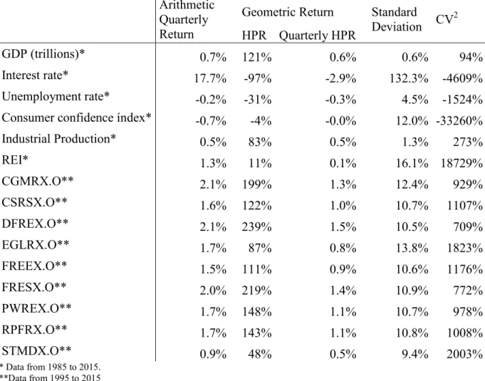
Table 4. Variables statistics.
Arithmetic Quarterly Return
Geometric Return Standard
Deviation CV2 HPR Quarterly HPR
GDP (trillions)* 0.7% 121% 0.6% 0.6% 94%
Interest rate* 17.7% -97% -2.9% 132.3% -4609%
Unemployment rate* -0.2% -31% -0.3% 4.5% -1524%
Consumer confidence índex* -0.7% -4% -0.0% 12.0% -33260%
Industrial Production* 0.5% 83% 0.5% 1.3% 273% REI* 1.3% 11% 0.1% 16.1% 18729% CGMRX.O** 2.1% 199% 1.3% 12.4% 929% CSRSX.O** 1.6% 122% 1.0% 10.7% 1107% DFREX.O** 2.1% 239% 1.5% 10.5% 709% EGLRX.O** 1.7% 87% 0.8% 13.8% 1823% FREEX.O** 1.5% 111% 0.9% 10.6% 1176% FRESX.O** 2.0% 219% 1.4% 10.9% 772% PWREX.O** 1.7% 148% 1.1% 10.7% 978% RPFRX.O** 1.7% 143% 1.1% 10.8% 1008% STMDX.O** 0.9% 48% 0.5% 9.4% 2003% * Data from 1985 to 2015. **Data from 1995 to 2015
GDP was around the 7.47 trillion of US dollars in 1985, and increased 121% until 2015 with the lowest standard deviation (0.6%). Industrial production index is also quite similar to the GDP, having a strong increasing tendency and low standard deviation. On the contrary, there are two variables with decreasing tendency: interest rate and unemployment, and although the first one is a lot more volatile (132.3%) than the second one (4.5%), it is able to averagely yield 17.7% of returns, which in terms of changes in our model has an enormous impact: high positive changes are expected. The variable with highest shifts and lowest
20 change in their value is the consumer confidence index, resulting in the heaviest coefficient of variation (-33260%). The last thing to note is that one of the main objectives in this project is to identify potential returns associated with the real estate through REITs, therefore it is important to mention that their quarterly average return is 1.05%, which was computed considering the HPR since the beginning of 1995, hence a compounded return. We also see that their arithmetic averages are slightly higher, however, the standard deviation is high, resulting in an averaged coefficient of variation of 1167% (average standard deviation of 11.1%), meaning that it is crucial to identify the correct quarters to invest, since a long term investment will most likely suffer from risk being ten times higher than return.
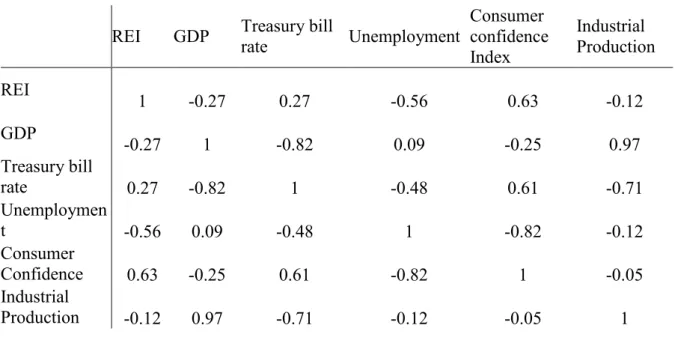
We also want to study the variables relationships, and the next table presents the correlations calculated from data starting in 1985. These are computed based on the well-known Pearson (1896) correlation coefficient for a sample.
Table 5. Economic variables correlations.
REI GDP Treasury bill rate Unemployment Consumer confidence Index Industrial Production REI 1 -0.27 0.27 -0.56 0.63 -0.12 GDP -0.27 1 -0.82 0.09 -0.25 0.97 Treasury bill rate 0.27 -0.82 1 -0.48 0.61 -0.71 Unemploymen t -0.56 0.09 -0.48 1 -0.82 -0.12 Consumer Confidence 0.63 -0.25 0.61 -0.82 1 -0.05 Industrial Production -0.12 0.97 -0.71 -0.12 -0.05 1
We want to avoid a certain level of multicollinearity, meaning that if two or more variables are too similar when trying to explain a dependent variable, it may influence the results, since the model will likely lean to choose one of them, neglecting the others. In that case, those in that situation should be dropped in order to get more significant results and a consistent model. As it can be seen in the previous table, the industrial production index has very high correlation with GDP, which is important to know a priori, as it may be pertinent to drop one of them during the investigation.
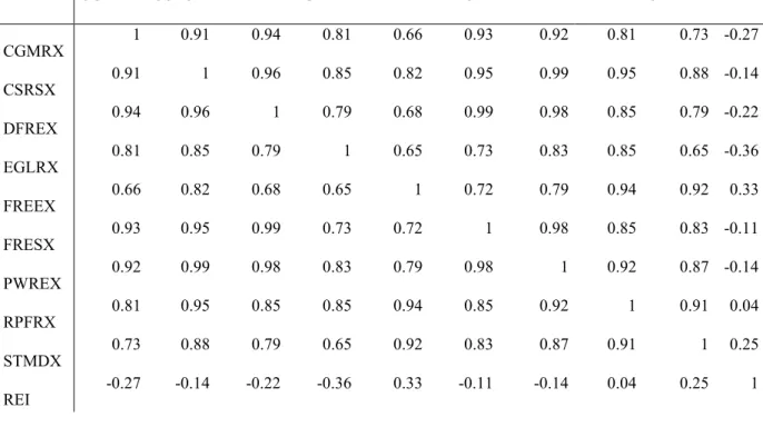
21 Although REITs are going to be in the left hand side of the equation, making the multicollinearity issue indifferent, table 6 also shows correlations between them, because we expect to analyze the results all together further in this investigation, and therefore we can avoid repeated results. In addition, this is important to prove that our dependent sample consistently reflects what happens in that market, by moving all in the same direction. This way, we can identify any drastically different REIT, which had to be independently considered. Among REITs, correlation varies between [0.65;0.99], which is indicative of a very strong correlation range, a part from the Real Estate Index, which may be explained by their different nature (the first is an investment vehicle, the second translates the people confidence in the sector, resulting in different evolution paces).
Table 6. 9 REITs group and REI correlations table.
CGMRX CSRSX DFREX EGLRX FREEX FRESX PWREX RPFRX STMDX REI
CGMRX 1 0.91 0.94 0.81 0.66 0.93 0.92 0.81 0.73 -0.27 CSRSX 0.91 1 0.96 0.85 0.82 0.95 0.99 0.95 0.88 -0.14 DFREX 0.94 0.96 1 0.79 0.68 0.99 0.98 0.85 0.79 -0.22 EGLRX 0.81 0.85 0.79 1 0.65 0.73 0.83 0.85 0.65 -0.36 FREEX 0.66 0.82 0.68 0.65 1 0.72 0.79 0.94 0.92 0.33 FRESX 0.93 0.95 0.99 0.73 0.72 1 0.98 0.85 0.83 -0.11 PWREX 0.92 0.99 0.98 0.83 0.79 0.98 1 0.92 0.87 -0.14 RPFRX 0.81 0.95 0.85 0.85 0.94 0.85 0.92 1 0.91 0.04 STMDX 0.73 0.88 0.79 0.65 0.92 0.83 0.87 0.91 1 0.25 REI -0.27 -0.14 -0.22 -0.36 0.33 -0.11 -0.14 0.04 0.25 1
22 4. Methodology
4.1 Choosing the best model
We are looking forward to investigating a viable way to explain returns in real estate using economic cycles, and to do it so we apply different methodologies to confirm their explanatory viability and possibly use them in the future, which are based on the methodology of multiple regression equation as explained by Kleinbaum, Kupper, Nizam, & Rosenberg (1998, pp. 141-148). We do regressions using the OLS method in the following equations, in order to compute the coefficients associated to the macroeconomic variables and their standard errors. There are a few testing processes which they have to pass through and apart from the next criteria, variables must also be independent, according to the previous autors. The regressions used are the BLUE of coefficients, meaning we compute them with the lowest variance possible, if the regression error term 3 follows several parameters:
- no evidence of serial correlation, meaning there should not be correlation throughout periods t among the errors, which is usually present before adding the lagged dependent variable in the regression, a common process used to clear trends as explained by Mills (1991, pp. 40-50) and it can be confirmed with Breusch-Godfrey LM test with 2 lag specification;
- normally distributed, which can be confirmed using Jarque-Bera test since errors’ skewness and kurtosis are used in JB test statistic with a chi-squared distribution with two degrees of freedom, whence the null hypothesis is skewness equalling to 0 and kurtosis to 0 or 3;
- with finite variance, which should keep stabilized as variables increase, otherwise the null hypothesis of homoskedasticity is rejected by Breusch-Pagan-Godfrey test. One of the common practices is to use logistic regressions which consist of putting variables under logarithm influence, thus providing a different interpretation of results, and it helps in some cases by giving a different overview. Instead of what happens in the direct linear relation, its results are not direct multiplicative coefficients, but probabilities of outcomes, and as explored by Pohlman and Leitner (2003), one should not be concerned to use them when testing relationships. Another common practice is
23 to use the Huber-White consistent covariance method, conditionally assuming homoskedasticity and therefore returning robust standard errors, since it only questions the coefficients significance without changing the coefficients themselves. This way, if they remain significant even if the errors previously were heteroskedastic, the analysis is validated (Huber, 1967), (Eicker, 1967) and (White, 1980).
4.1.1 Real estate index
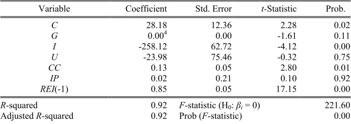
It is important to mention that the key point is to establish a relationship with a cyclic variable, thus making it theoretically possible to work within different time spans (Burns & Mitchel, 1946). So, the first method has a different starting period (first quarter of 1985) than the later ones, because the dependent variable has older monitoring. The equation follows:
( 2 ) where REI stands for real state index, G for GDP, I for the US 3-month Treasury bill rate, U for unemployment rate, CC for consumer confidence index and IP for industrial production index. stands for the constant variable, β stand for the coefficients and ε is the error term representation. In addition, we added a new variable to face the serial correlation problem, which is equal to the dependent variable REI except for being lagged 1 period. Table 7. Real estate index regression.
Sample (adjusted): 6/01/1985 12/01/2015 Included observations: 123 after adjustments
Variable Coefficient Std. Error t-Statistic Prob.
C 28.18 12.36 2.28 0.02 G 0.004 0.00 -1.61 0.11 I -258.12 62.72 -4.12 0.00 U -23.98 75.46 -0.32 0.75 CC 0.13 0.05 2.80 0.01 IP 0.02 0.21 0.10 0.92 REI(-1) 0.85 0.05 17.15 0.00 R-squared 0.92 F-statistic (H0: βi = 0) 221.60
Adjusted R-squared 0.92 Prob (F-statistic) 0.00
24 After complying with all requirements of having normally distributed residuals value: 0.25 > 0.05), not serially correlated value: 0.14 > 0.05) and not heteroskedastic (p-value: 0.17 > 0.05), we conclude that 3-month Treasury bill rate (p-(p-value: 0.00 < 0.05) and consumer confidence (p-value: 0.01 < 0.05) are the main variables that explain real estate index, as well as the model has quite strong R-squared (0.92) and a significant F-statistic (p-value: 0.00 < 0.05) (see table 7). However, these results are merely indicative of potential relationships with real estate market, since our dependent variable is not a profitable investment instrument, but a confidence index representative of population’s sentiment.
4.1.2 REITs returns
The previous evidence leads us to use REITs. First possibility is to directly use returns, and investigate how much they can be explained by macro variables. The time span is now from 1995 to 2015. The already explained selection of 9 REITs is used in the second methodology in order to compute averagely the returns, so that the dependent variable has lower dependency on unsystematic risk (which could be driven by poor management of a few REITs). Also, the average is a common measure to all REITs, whether they have different size NAVs or not. Therefore, equation 3 reflects its regression:
( 3 ) where in this case REIT5 represents the returns in each period t, the dependent variable includes the average of (n = 9) pre-selected REITs, G stands for the Gross Domestic Product,
I for the interest rates, U for unemployment rate, and CC for consumer confidence and IP for
the industrial production. stands for the constant variable, the β for the coefficients and ε is the error term representation. All explanatory variables reflect the change from period t – 1 to
t weighted by their value in t - 1, to be in accordance with REITs returns.
5
, where i stands for each of the n = 9 REITs in each t period. stands for the portfolio quarterly averaged returns (see equation 1 for the returns computation).
25 Table 8. REITs returns regression.
Sample: 3/01/1995 12/01/2015 Included observations: 84
Variable Coefficient Std. Error t-Statistic Prob.
C -0.003 0.01 -0.23 0.82 REI 0.08 0.06 1.31 0.19 G 2.36 1.85 1.27 0.21 I 0.0006 0.01 0.10 0.92 U 0.16 0.24 0.64 0.51 CC 0.39 0.09 4.37 0.00 IP -0.80 0.84 0.95 0.34 R-squared 0.41 F-statistic (H0: βi = 0) 8.83
Adjusted R-squared 0.36 Prob (F-statistic) 0.00
After conducting the residuals tests, and although the errors are not heteroskedastic value: 0.08 > 0.05), not serial correlated value: 0.67 > 0.05) and normally distributed (p-value: 0.99 > 0.05), we cannot affirm that variables strongly explain the REITs’ returns in the markets, since it has a R-squared of 0.41, and the variables are not statistically significant, except for consumer confidence index (p-value: 0.00 < 0.05). Industrial production index (negative coefficient: -0.80) seems to work inversely against the funds’ returns, as well as unemployment (positive coefficient: 0.16) which it is economically discouraging but may contribute positively to them. This results from the model multivariable construction, as separated tests were conducted exclusively with industrial production index and unemployment rate, and they worked in their normal way: industrial production index coefficient was positive and intercept negative; unemployment was also positive but with a high positive intercept value (which indicates that if unemployment were 0, returns would be positive).
.1.3 REITs NAV
It is possible that regressing returns (a variable that varies between positive and negative values) against the economical variables changes limits our possibilities to work with regression transformations like logarithms and square roots. However, there is the solution of
26 using NAV per share6, a common pricing tool in these markets, instead of computing returns. This way, we ensure that the dependent variable is more similar to the explanatory ones and we are able to try different approaches to smoothen the variables dimension. And because an average of all NAV per share would not be suitable, as they are heterogeneous with different sizes, we decided to independently use the 9 REITs in regressions and compare the results. Therefore, we used equation 4:
( 4 ) where REIT represents each of 9 REIT NAV in each period t, G stands for the Gross Domestic Product, I for the interest rates, U for unemployment rate, and CC for consumer confidence and IP for the industrial production. stands for the constant variable, the β for the coefficients and ε is the error term representation (see in the appendices section, tables 17 to 25). Due to serial correlation in all 9 cases, it was added the REIT lagged variable to correct it. Furthermore, there were also arising non-normality problems among the errors, mainly because of the new addition, so, after different attempts, logarithmic transformation of all variables was the most viable way to dissipate them. Besides, there was still heteroskedasticity evidence, so we decided to use robust standard errors from coefficients, questioning their statistical significance, although the coefficients themselves remained unchanged. In the end, there was only one REIT7 violating the criteria because of its non-normal distributed residuals, but since all of them showed consistency in this matter, and several authors like Kupper, Nizam, & Rosenberg (1998), Lumley, Diehr, Emerson, & Chen (2002) and Stuart, Ord, & Arnold (1999) claim that it is not as critical as other assumptions. Regarding normality in residuals, the first ones wrote “... only extreme departures of the distribution of Y [dependent variable] from normality yield spurious results” and the second ones added “This is consistent with the fact that the Central Limit Theorem is more sensitive to extreme distributions in small samples, as most textbook analyses are of relatively small
6 According to the US SEC, NAV translates “the company's total assets minus its total liabilities. Mutual funds and Unit Investment Trusts (MUITs) generally must calculate their NAV at least once every business day, typically after the major U.S. exchanges close.”
27 sets of data”. To conclude, after the previous considerations, this may eventually be a sample size issue, which would disappear if we increased the observations number. Coefficients and respective significance are disposed in table 9, as well as their average.
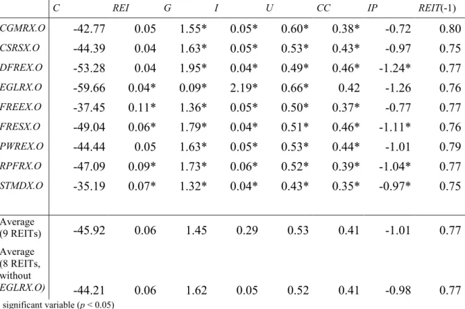
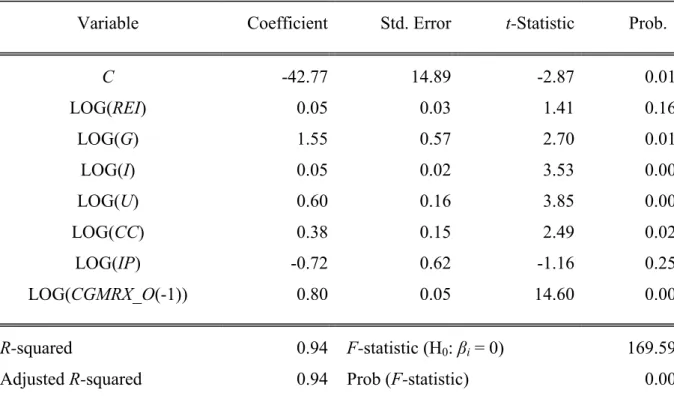
Table 9. Equation 4 coefficients and corresponding significance.
C REI G I U CC IP REIT(-1) CGMRX.O -42.77 0.05 1.55* 0.05* 0.60* 0.38* -0.72 0.80 CSRSX.O -44.39 0.04 1.63* 0.05* 0.53* 0.43* -0.97 0.75 DFREX.O -53.28 0.04 1.95* 0.04* 0.49* 0.46* -1.24* 0.77 EGLRX.O -59.66 0.04* 0.09* 2.19* 0.66* 0.42 -1.26 0.76 FREEX.O -37.45 0.11* 1.36* 0.05* 0.50* 0.37* -0.77 0.77 FRESX.O -49.04 0.06* 1.79* 0.04* 0.51* 0.46* -1.11* 0.76 PWREX.O -44.44 0.05 1.63* 0.05* 0.53* 0.44* -1.01 0.79 RPFRX.O -47.09 0.09* 1.73* 0.06* 0.52* 0.39* -1.04* 0.77 STMDX.O -35.19 0.07* 1.32* 0.04* 0.43* 0.35* -0.97* 0.75 Average (9 REITs) -45.92 0.06 1.45 0.29 0.53 0.41 -1.01 0.77 Average (8 REITs, without EGLRX.O) -44.21 0.06 1.62 0.05 0.52 0.41 -0.98 0.77 * significant variable (p < 0.05)
From this last process, we conclude that, for R’s-squared within [0.89;0.95] (which represents good estimating models), there are several variables with maximum evidence of significance: GDP, US 3-month Treasury bill rate and unemployment. Besides, the consumer confidence index also must be taken into consideration due to being almost every time significant. These results led to the generation of a new model, constrained to the most relevant variables: the previous four. The new formulation and results follow (see in the appendices section, tables 26 to 34):
28 Table 10. Equation 5 coefficients and corresponding significance.
C G I U CC REIT(-1) CGMRX -28.07 0.96* 0.04* 0.65* 0.42* 0.80 CSRSX -26.09 0.89* 0.04* 0.59* 0.45* 0.74 DFREX -28.89 0.97* 0.03* 0.57* 0.45* 0.77 EGLRX -37.48 1.29* 0.08* 0.75* 0.43* 0.74 FREEX -18.10 0.60* 0.03* 0.56* 0.49* 0.81 FRESX -26.53 0.89* 0.03* 0.58* 0.49* 0.77 PWREX -24.63 0.83* 0.03* 0.60* 0.46* 0.78 RPFRX -25.68 0.86* 0.04* 0.59* 0.48* 0.77 STMDX -14.42 0.49* 0.03* 0.49* 0.40* 0.78 Average (9 REITs) -25.54 0.86 0.04 0.60 0.45 0.77 Average (6 REITs, without CSRSX, EGLRX and RPFRX) -23.44 0.79 0.03 0.58 0.45 0.79 * significant variable (p < 0.05)
This reformulation allowed the model to be more consistent, since all four explanatory variables remained significant, imperfect variables were excluded and the model kept good
R’s-squared [0.87;0.95]. Also, the same procedures previously applied regarding the residuals
were tested, making REITs to become serially uncorrelated, coefficients to remain significant with robust standard errors and residuals to be normally distributed (although 3 of them8 violated the last criterion, but as previously done, justified by the sample size). The averages are also computed, and are going to be the main reference onwards, knowing that little difference results from excluding the 3 REITs.
4.2 Testing the model
2.1 Scenarios analysis
In this section, we intend to analyze different scenarios to identify potential returns. In the situation that all independent variables increase 10% from the previous period, REITs’
8 CRSRX.O (Cohen & Steers Realty Shares Mutual Fund); EGLRX.O (Alpine International Real Estate Equity Fund Institutional); RPFRX.O (Davis Real Estate Fund A)
29 returns will increase 19.24%9. However, as it is explained later, it does not make sense to verify an increase in all economic variables, since unemployment evolves inversely to the others. Therefore, the following table represents different realistic scenarios, with each variable change in the left (inverse changing in the unemployment case) and the output to REITs in the right:
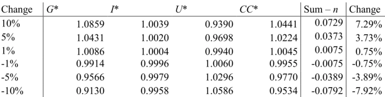
Table 11. Scenarios with changes and REITs output.
Change G* I* U* CC* Sum – n Change
10% 1.0859 1.0039 0.9390 1.0441 0.0729 7.29% 5% 1.0431 1.0020 0.9698 1.0224 0.0373 3.73% 1% 1.0086 1.0004 0.9940 1.0045 0.0075 0.75% -1% 0.9914 0.9996 1.0060 0.9955 -0.0075 -0.75% -5% 0.9566 0.9979 1.0296 0.9770 -0.0389 -3.89% -10% 0.9130 0.9958 1.0586 0.9534 -0.0792 -7.92%
*the change of each variable j was computed with the formula: , where p represents the change, and β the
coefficient.
The previous table shows that changes in economy do not strongly affect REITs, although it has a clear impact. For instance, if the economy grows 5% (which was the increase in GDP from 2014 to 2016), it results in an expected increase of 3.73% in REITs. This kind of analysis allows using these vehicles as diversifying investments, since they themselves usually have several investments in hedging instruments, which may be the reason behind low impact from economy10 (Beyene, Fisher, & Schachat, 2015). The main issue which has to be considered in these scenarios is the likelihood of those changes in each variable. In order to assess it, next table presents the average, standard deviation, maximum and minimum values computed from changes in the variables throughout periods, so that it is foreseeable the kind of scenarios are more likely to happen, and the weight to allocate to each of them.
9
, where β represents the variables’ coefficients and n = 4.
, where p = 10%
10 REITs’ funds commonly hedge by investing in derivatives (like swaps or futures), and balancing their focus in the real estate sector. Although they have to pass through several tests and comply with specific rules (95% and 75% of gross income derived from specific real property related sources and others, according to Code Secs. 856(c)(2) and 856(c)(3) respectively), hedging investment will be protected in real estate focus tests by their own rules after evaluated “its compliance with all of the requirements of the hedging rules of Code Secs. 856(c)(5)(G) and 1221(a)(7) to determine the treatment of any income derived from the hedges under the REIT income tests”, thus being excluded from those percentages (Beyene, Fisher, & Schachat, 2015).
30 Table 12. Statistical measures from changes in explanatory variables.
From 1995 to 2015 G I U CC REIT(-1) Geometric Average 0.59% -3.80% -0.11% -0.05% 1.05% Std. Deviation11 0.63% 161.21% 4.98% 12.22% 11.10% Maximum 1.89% 1050.00% 20.39% 61.72% 63.76% Minimum -2.11% -97.35% -7.50% -28.93% -44.96%
GDP is (by far) the variable whose changes in each period are less volatile, thus making it less likely changes of 10%, since in 30 years, the maximum value was 1.89%, and its standard deviation is very low (0.63%). On contrast, the interest rate is the one with higher expected impact in the model, since its average is quite negative and high (-3.80%), and an extreme standard deviation of 161.21%. These previous variables have their discrepant results mainly due to their different sizes, leading to less significant changes in GDP case and more significant ones in the Treasury bill case. Furthermore, it is also important to consider unemployment and consumer confidence, whose averages are -0.11% and -0.05% (respectively), but yielding higher standard deviations than GDP. The lagged REIT values were computed from the 9 REITs sample, and despite not explaining economically anything, they have to be considered in the sum of all changes.
To conclude, using the average values of changes from last table, we can compute the expected change in REITs once more. Since we are working with averages, we assume they reflect a common situation, which would quarterly yield 1.08%12 of change in REITs and an annually compounded yield of 4.40%. Having this in mind, one could seize opportunities through investment in real estate economy at the right times. As it was previously mentioned, the economy is cyclic, and in times of expected expansion, it is even worthier to invest in REITs by relying on the variables predicted changes, whilst some assumptions hold: - the random process of choosing a portfolio instead of one or two REITs avoids investing only in specific ones, which could dramatically overload the process with unsystematic risk driven from poor management; - investing only in American REITs; - the predictions to the investment period are correct.
11 Computed considering geometric average. 12
, where β represents the variables’ coefficients and n = 5. , where p is the average change in each j variable.
31 4.2.2 Enlarging the sample
Enlarging the sample is one of the ways to verify the consistency of results obtained by the previous data. Therefore, we decided to start 5 years later (in 2000), granting information about 3013 REITs instead of only 9. We apply the equation of what we conclude to be the best model (equation 5), and the next table shows the results.
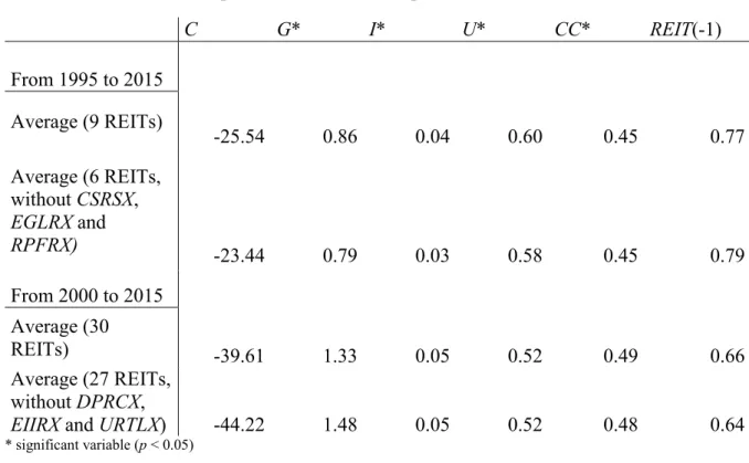
Table 13. Coefficients comparison of different samples.
C G* I* U* CC* REIT(-1) From 1995 to 2015 Average (9 REITs) -25.54 0.86 0.04 0.60 0.45 0.77 Average (6 REITs, without CSRSX, EGLRX and RPFRX) -23.44 0.79 0.03 0.58 0.45 0.79 From 2000 to 2015 Average (30 REITs) -39.61 1.33 0.05 0.52 0.49 0.66 Average (27 REITs, without DPRCX,
EIIRX and URTLX) -44.22 1.48 0.05 0.52 0.48 0.64
* significant variable (p < 0.05)
The first thing to mention is that all variables are significant and comply with the requirements, except for three REITs and once again we have to remove them from the equation, mainly because GDP is not significant in the regression model in those cases. However, we investigate the reasons behind it, and conclude that those REITs are in fact the ones with higher variation coefficients ratios, meaning that their performances are very different from the other ones, which is most likely driven by poor management. From the table, we conclude that all variables remain quite similar, whose changes are around the interval of [0,02;0,11], except for the intercept (from -25.54 to 39.61) and the GDP (from 0.86 to 1.33), whose coefficients show an higher impact, increasing the leverage on this economic
13 Since 2000 there were new REITs available to join the initial 9. However, some were left behind because of having too high correlation levels, above 0.99, as result of being from the same institution and probably under the same management. After identifying them, the selection process was random, leaving 11 out of the analysis.
32 variable. This way, we take into consideration that GDP may be the variable with extra unpredictable impact on our model, which means that if GDP increases or decreases in one period, it may influence the returns more than the previously predicted.
4.3 Identifying the ideal periods
We are looking for the best periods to invest, hence periods with higher returns and higher residuals, as the second condition allows beating the expectations14. This is a secondary goal, but important to bear in mind in order to mitigate the possibility of unexpected losses. The next table shows what we considered the best moments, with respective aggregated returns and residuals, being very clear the best opportunities to invest: from June-95 to September-97, from March-03 to March-07 and from June-09 to June-13. The periods were defined after aggregating the results in several attempts in order to obtain optimized selections with a reasonable amount of time (2 to 5 years).
Table 14. Aggregated periods, returns and residuals. REITs
Average Jun-95 to Set-97 Dez-97 to Dez-02 Mar-03 to Mar-07 Jun-07 to Mar-09 Jun-09 to Jun-13 Set-13 to Dez-15
Actual Return 44% -8% 80% -106% 116% 12%
Fitted Return 39% 3% 74% -93% 107% 3%
Quarterly
Average 4.4% -0.3% 4.7% -13.25% 6.82% 1.2%
Residual Sum 0,50 -1,00 0,69 -0,32 -0,13 0,27
Note: REITs quarterly yield 1.05%.
First immediate concern to discuss is that the periods have different lengths. However, we believe that some months before June-95 would follow the same pattern, resulting from the recovery since 1990-91. The same idea would apply to the months following December-2015, since these two periods are shorter than the others. The last period to consider in this
14 where represents regressions expected values and the actual values. appears in the function as logarithm of NAV.
33 situation is the crisis from June-07 to March-09 which stroke very rapidly and brutally, resulting in a shortened duration. Nevertheless, it is clear the differences among performances, being the ideal periods not only more profitable, but also capable of avoiding the turbulent times, generating up to at least four times the normal return (4.40%).
Regarding the prediction matter, the cycles are not always the same, and the next graphs give an idea of it through the Hodrick-Prescott filter application to the variables. It allows detrending time series, returning a smoother estimate, but also the cycle component, being easier to understand the seasonal effect in each cycle. Bars show the aggregated periods division.
Graph 3. GDP after HP filter (quarterly, λ = 1600).
-0,040 -0,030 -0,020 -0,010 0,000 0,010 0,020 0,030 mar-95 mar-15 Lo g( G) cy cle co m po nen t Year
34 Graph 4. 3-month Treasury bill rate after HP filter (quarterly, λ = 1600).
Graph 5. Unemployment rate after HP filter (quarterly, λ = 1600). -3 -2 -1 0 1 2 3 mar-95 mar-15 Lo g( I) cy cle co m po nen t Year -0,3 -0,2 -0,1 0 0,1 0,2 0,3 mar-95 mar-15 Lo g( U) cy cle co m po nen t Year
35 Graph 6. Consumer confidence index after HP filter (quarterly, λ = 1600).
Firstly, the graphs only reveal the cycle component, meaning that even if it is negative, variables might increase, caused by their long-term trend components.
GDP is the only variable with steady increasing evolution (very clear trend), having only one drawback during the crisis, so one can expect almost always increases, however sometimes more significant than others. According to its cycle, it is preferable to invest during the recovery period, hence after deep falls, with duration from 2 to 4 years. In addition, if positive changes slow down, it will be a signal of the recovery period end.
The interest rate has decreased since 1980 (see in the appendices section, graph 7) until these days, however it has not been in a linear way, because of the upward parts in the cycle component (graph 4) which balance the decreasing trend. Although this may be the variable with the most difficult relationship to identify, we see a similar pattern to the GDP. We have also to consider that it is logged, returning too negative values when interest rates are too low. This overpowers the real impact into the model, because REITs profitability did not change much in function of interest rates once they were fixed very closed to zero (in 2009).
Regarding the unemployment rate, we have to consider its inertia, as it was previously discussed to take more time to recover in the beginning of the expansion. This is one of the reasons why it is a good explanatory variable, since the economy is already walking in the right direction and showing good expectations, whereas the unemployment is still increasing
-0,800 -0,600 -0,400 -0,200 0,000 0,200 0,400 mar-95 mar-15 Lo g( C C ) cy cle co m po nen t Year
36 or stabilizing instead of decreasing (which is not necessarily armful, when in fact the results are very promising to the investment during that time). At a regression level, it works as a different variable, and the unemployment graph shows that it is important to take advantage exactly when it reaches the peak of that cycle, meaning that (even though at a high level) the best moment already began.
The consumer confidence index is also similar to GDP, as its cycle component increases since the beginning of 1993, changing its direction around the second considered period, although it is not very clear. The other periods follow the same logic to invest, however this variable is more volatile; an issue that does not affect the model.
37 Conclusion
This project proves the existence of potential returns in a consistent way in the real estate market. Looking back to the literature review, it is already known that GDP, consumer confidence index and 3-month Treasury bill interest and unemployment rates are good references of the economic cycle. In the same way, the first one is the most used to measure the cycle, unemployment rate is known for its delayed reaction, and interest rates are quite unpredictable. Still, we discovered how these four variables serve as a valuable joint input in the particular case of explaining real estate, as well as industrial production index and real estate index will not produce added value to the equation. REITs share a low correlation with real estate indices (which are based on population confidence) in a quarterly basis, and these are less appropriate to be the proxy for the investment in real estate. On contrast, REITs are a good substitute to measure the investment in this economic approach as a result of their flexible nature; however the best way to analyze their performance is not through returns, rather through NAV. In addition, this is supported by three pillars: change in the economy, liquidity and diversification.
Our results prove through a consistently significant econometric model that when the economy attains better results in the following quarter, there are positive returns in the REITs market; on the opposite side, if it is predicted either a slowdown or a decline, the position will suffer. This market yields 4.40% of returns on yearly average, but we have seen that it will return at least that amount quarterly if one selects the right periods: mainly the recovery periods right after huge crisis or slowdowns. Moreover, investing in open-end funds, a type of funds characterized by ensuring a high level of liquidity through the constant possibility of issuing and re-buying investors shares, avoids holding leveraged investments in the long term (like the properties themselves), thus offering an exit strategy. As we analyze in the beginning of the research (Devos, Ong, Spieler, & Tsang, 2013), we know that institutional investors tend to have long positions in times prior to crises, and that is another reason to close the position in the second half of the cycle expansion period, as demand and investment are higher and it will be easier to redeem our shares.
38 6. Appendices
Graph 7. 3-month Treasury bill rate since 1970.
Graph 8. Unemployment rate after HP filter since 1970 (quarterly, λ = 1600). 0,00% 2,00% 4,00% 6,00% 8,00% 10,00% 12,00% 14,00% 16,00% 18,00%
mar-70 mar-75 mar-80 mar-85 mar-90 mar-95 mar-00 mar-05 mar-10 mar-15
In ter est r ate Year -0,3 -0,2 -0,1 0 0,1 0,2 0,3 0,4
mar-70 mar-75 mar-80 mar-85 mar-90 mar-95 mar-00 mar-05 mar-10 mar-15
Lo g( U) cy cle Year
39 Table 15. Official definitions of sectors and investment instruments. Information from the NAICS.
NAICS Code Description
Real estate sector 531 Industries in the Real Estate subsector
group establishments that are primarily engaged in renting or leasing real estate to others; managing real estate for others; selling, buying, or renting real estate for others; and providing other real estate related services, such as appraisal services. This subsector includes equity Real Estate Investment Trusts (REITs) that are primarily engaged in leasing buildings, dwellings, or other real estate property to others. Mortgage REITs are classified in Subsector 525, Funds, Trusts, and Other Financial Vehicles.
Open-end investment funds 525910 This industry comprises legal entities (i.e., open-end investment funds) organized to pool assets that consist of securities or other financial instruments. Shares in these pools are offered to the public in an initial offering with additional shares offered continuously and perpetually and redeemed at a specific price determined by the net asset value.
Mortgage REITs 531110 This industry comprises legal entities
(i.e., funds (except insurance and employee benefit funds; open-end investment funds; trusts, estates, and agency accounts)). Included in this industry are mortgage Real Estate Investment Trusts (REITs).