Cálculo fraccional em escalas temporais

(1)

!"#!

**$%&'()+,-(.,**

**/-01,02(345'4**

6&01,240.*.,(.,(71,02'!"#$%&'%(#)'*!+#!,%'#(-'./%

**89-:%-'(;2::0'&-(,<(=4:-4(>,<?'2*04**

**;2:50'&-(8-:%-%4('&(>0<,(@:-,4**

0,%'1#(%'./%2! +.3/*4#&.#35! 3(%22! *& 6&#%'5!%&#!)#4#&!7*&)!*8!3$*)'%)#*93 6#)#&%'.*):!;1#<!%2=%<3!$&#39$$*3#!% 3*.2!3##+#+!=.'1!$&#2.(.)%&<!>)*=2#+6# %)+! =#22! $&#$%&#+! 7<! 2%7*9&5! 7*'1 /*)3/.*93!%)+!397/*)3/.*93:? @#)&.!A*.)/%&B

(2)

Universidade de Aveiro 2012

Departamento de Matemática

Nuno Rafael de

Oliveira Bastos

Cálculo Fraccional em Escalas Temporais

Fractional Calculus on Time Scales

Tese apresentada à Universidade de Aveiro para cumprimento dos requisitos necessários à obtenção do grau de Doutor em Matemática, Programa Doutoral em Matemática e Aplicações – PDMA 2007-2011– da Universidade de Aveiro e Universidade do Minho, realizada sob a orientação científica do Doutor Delfim Fernando Marado Torres, Professor Associado com Agregação do Departamento de Matemática da Universidade de Aveiro.

Thesis submitted to the University of Aveiro in fulfilment of the requirements for the degree of Doctor of Philosophy in Mathematics, Doctoral Programme in Mathematics and Applications – PDMA 2007-2011 – of the University of Aveiro and University of Minho, under the supervision of Professor Delfim Fernando Marado Torres, Associate Professor with tenure and Habilitation of the University of Aveiro.

Apoio financeiro do Instituto Politécnico de Viseu e da FTC (Fundação para a Ciência e Tecnologia) através do “Programa de apoio à formação avançada de docentes do Ensino

Superior Politécnico”, bolsa de

doutoramento com referência

SFRH/PROTEC/49730/2009.

(3)

Dedico esta tese aos meus pais, ao meu irmão e à Vanda pela força e pelo apoio incondicional que me deram ao longo destes anos.

(4)

o júri

presidente Prof. Doutor José Carlos da Silva Neves

Professor Catedrático da Universidade de Aveiro (por delegação do Reitor da Universidade de Aveiro)

Prof. Doutor Manuel Duarte Ortigueira

Professor Associado com Agregação da Faculdade de Ciências e Tecnologia da Universidade Nova de Lisboa

Prof. Doutor Delfim Fernando Marado Torres

Professor Associado com Agregação da Universidade de Aveiro (orientador)

Prof. Doutor Filipe Artur Pacheco Neves Carteado Mena

Professor Associado da Escola de Ciências da Universidade do Minho

Prof. Doutora Agnieszka Barbara Malinowska

Professora Auxiliar da Białystok University of Technology, Polónia

Prof. Doutor Ricardo Miguel Moreira de Almeida

(5)

Agradecimentos

acknowledgements

I would like to acknowledge my supervisor Delfim F. M. Torres for accepting me as his student. I could not imagine having a better supervisor because without his knowledge, invaluable guidance, advice, trust, encouragement and endless patience, I would never have finished this thesis.

I wish to express a special gratitude for the financial support of the Polytechnic

Institute of Viseu and the Portuguese Foundation for Science and Technology

(FCT), through the “Programa de apoio à formação avançada de docentes do Ensino Superior Politécnico”, PhD fellowship SFRH/PROTEC/49730/2009, without which this work wouldn’t be possible.

I’m thankful to the people, with whom I interacted, at the Department of Mathematics of University of Aveiro and at the Department of Mathematics of Faculty of Computer Science, Białystok University of Technology, for providing a kind atmosphere and to contribute, in some sense, to this work.

I also thank to my friends for their untiring support and to my department colleagues for their encouraging comments during these years, especially when this thesis seemed stopped.

I wish to thank to Vanda for her patience, never-ending support and for never allowing me feeling alone in this hard and long way, providing, on that sense, the perfect conditions to work on this thesis.

I also wish to express my deepest gratitude to my family for their invaluable support and for understanding my missing in several moments of this work. Finally, I wish to dedicate this thesis to my parents, to my brother and to Vanda.

(6)

palavras-chave Problemas variacionais fracionais em tempo discreto, operadores fracionais discretos do tipo de Riemann—Liouville, soma por partes fraccional, equações de Euler—Lagrange, condição necessária de optimalidade do tipo de Legendre, escalas temporais, sistema de computação algébrico Maxima.

resumo Introduzimos um cálculo das variações fraccional nas escalas temporais ℤ e (hℤ)_!. Estabelecemos a primeira e a segunda condição necessária de optimalidade. São dados alguns exemplos numéricos que ilustram o uso quer da nova condição de Euler–Lagrange quer da nova condição do tipo de Legendre. Introduzimos também novas definições de derivada fraccional e de integral fraccional numa escala temporal com recurso à transformada inversa generalizada de Laplace.

(7)

keywords Fractional discrete-time variational problems, discrete analogues of Riemann— Liouville fractional-order operators, fractional formula for summation by parts, Euler—Lagrange equations, Legendre type necessary optimality condition, time scales, Maxima computer algebra system.

abstract We introduce a discrete-time fractional calculus of variations on the time scales ℤ and (ℎℤ)_!. First and second order necessary optimality conditions are established. Some numerical examples illustrating the use of the new Euler— Lagrange and Legendre type conditions are given. We also give new definitions of fractional derivatives and integrals on time scales via the inverse generalized Laplace transform.

(8)

Introduction

The main goal of this thesis is to develop a more general fractional calculus on time scales.

In the first year of my PhD Doctoral Programme I followed several one-semester courses in distinct fields of mathematics. One of the one-semester courses was called Research Lab where five different subjects were covered. One of those subjects was calculus of variations on time scales. Time scales theory looked to me a new and wonderful subject. As the doctoral programme PDMA Aveiro–Minho is backed up by two research units, not only Professors of the first semester but any researcher that belongs to any of these R&D units is invited to present, at the end of the first semester, research topics for PhD thesis by giving seminars to interested students. The author’s supervisor was one of the researchers that was available to be advisor if any student show interest in the theme Fractional Calculus on Time Scales – the title of this thesis.

The main idea was to connect in one theory two subjects that were, and still are, subject to strong research and development. Our contribute on this new area, until now, appears in part II of this thesis. On one hand we develop a discrete fractional calculus of variations for the time scale Z (Chapter 3) and for the time scale (hZ)a (Chapter 4). One the other

hand we give new definitions for differintegral fractional calculus on a time scale using a Laplace transform approach (Chapter 5).

Nowadays fractional differentiation (differentiation of an arbitrary order) plays an im-portant role in various fields: physics (classic and quantum mechanics, thermodynamics, etc.), chemistry, biology, economics, engineering, signal and image processing, and control theory [8,60,72,73,87,94,95,100,108,110]. It is a subject as old as Calculus itself but much in progress [98]. The origin of fractional calculus goes back three centuries, when in 1695 L’Hopital asked Leibniz what should be the meaning of a derivative of order 1/2. Leibniz’s response: “An apparent paradox, from which one day useful consequences will be drawn”.

(11)

INTRODUCTION

After that episode, which most authors consider the born of fractional calculus, several fa-mous mathematicians contributed to the development of Fractional Calculus [60, 87, 108]: Abel, Fourier, Liouville, Grünwald, Letnikov, Caputo, Riemann, Riesz, just to mention a few names. In the last decades, considerable research has been done in fractional calculus. This is particularly true in the area of the calculus of variations, which is being subject to intense investigations during the last few years [11, 25, 26, 92, 102, 103]. F. Riewe [105, 106] obtained a version of the Euler-Lagrange equations for problems of the calculus of varia-tions with fractional derivatives, that combines the conservative and non-conservative cases. In fractional calculus of variations our main interest is the study of necessary optimality conditions for fractional problems of the calculus of variations. The study of fractional problems of the calculus of variations and respective Euler–Lagrange equations is a fairly recent issue – see [3, 4, 6, 7, 10, 14, 26, 49, 50, 55, 56, 91] and references therein – and include only the continuous case. It is well known that discrete analogues of differential equations can be very useful in applications [28, 68, 71] and that fractional Euler-Lagrange differen-tial equations are extremely difficult to solve, being necessary to discretize them [6, 26]. Therefore, we consider pertinent to develop a fractional discrete-time theory of the calculus of variations in a different time scale than R. We dedicate two chapters to that: one for the time scale Z and another for the time scale (hZ)a. Applications of fractional calculus

of variations include fractional variational principles in mechanics and physics, quanti-zation, control theory, and description of conservative, nonconservative, and constrained systems [25, 30, 31, 103]. Roughly speaking, the classical calculus of variations and optimal control are extended by substituting the usual derivatives of integer order by different kinds of fractional (non-integer) derivatives. It is important to note that the passage from the integer/classical differential calculus to the fractional one is not unique because we have at our disposal different notions of fractional derivatives. This is, as argued in [25, 102], an interesting and advantage feature of the area. Most part of investigations in the fractional variational calculus are based on the replacement of the classical derivatives by fractional derivatives in the sense of Riemann–Liouville, Caputo and Riesz [3, 10, 15, 25, 57, 93]. In-dependently of the chosen fractional derivatives, one obtains, when the fractional order of differentiation tends to an integer order, the usual problems and results of the calculus of variations.

A time scale is any nonempty closed subset of the real line. The theory of time scales is a fairly new area of research. It was introduced in Stefan Hilger’s 1988 Ph.D. thesis [61]

(12)

INTRODUCTION

and subsequent landmark papers [62,63], as a way to unify the seemingly disparate fields of discrete dynamical systems (i.e., difference equations) and continuous dynamical systems (i.e., differential equations). His dissertation referred to such unification as “Calculus on Measure Chains” [24, 75]. Today it is better known as the time scale calculus. Since the nineties of XX century, the study of dynamic equations on time scales received a lot of attention (see, e.g., [2, 41, 43]). In 1997, the German mathematician Martin Bohner came across time scale calculus by chance, when he took up a position at the National University of Singapore. On the way from Singapore airport, a colleague, Ravi Agarwal, mentioned that time scale calculus might be the key to the problems that Bohner was investigating at that time. After that episode, time scale calculus became one of its main areas of research. To the reader who wants a gentle overview of time scales we advise to begin with [111], that was written in a didactic way and at the same time points some possible applications (e.g. in biology). Here we are interested in the calculus of variations on time scales [85, 112]. Our goal is to connect the theories of calculus of variations on time scales and fractional calculus.

This thesis is divided in two major parts. The first part has two chapters in which we provide some preliminaries on fractional calculus and time scales calculus, respectively. The second part is splitted in three chapters where we present our original work. In Chapter 3 we introduce the fractional calculus of variations on the time scale Z. The main results of this chapter are a first-order necessary optimality condition (Euler-Lagrange equation) and a second-order necessary optimality condition (Legendre inequality). In Chapter 4 we introduce a fractional factorial function that allow us to define left and right fractional derivatives and to develop further the two necessary optimality conditions of Chapter 3. In Chapter 4 the time scale is hZa. We believe that our results open some possible doors

to research, also in the continuous case, when h → 0. Chapter 5 is devoted to a new approach to define fractional derivatives and fractional integrals in an arbitrary time scale, by using the Laplace transform of time scales as support. Finally, we write our conclusions in Chapter 6 as well some future research directions.

(13)

(14)

Part I

Synthesis

(15)

(16)

Chapter 1 Fractional Calculus

“The fractional calculus is the calculus of the XXI-st century” K. Nishimoto (1989) The theory of discrete fractional calculus is in its infancy [20, 21, 86]. In contrast, the theory of continuous fractional calculus is much more developed [108]. The fractional discrete theory has its foundations in the pioneering work of Kuttner in 1957, where it appears the first definition of fractional order differences. In Sections 1.1 and 1.2 some definitions of fractional discrete and continuous operators are given, respectively.

1.1 Discrete fractional calculus

In 1957 [74] Kuttner defined, for any sequence of complex numbers,{an}, the s-th order

difference as ∆san = ∞ ! m=0 "−s − 1 + m m # an+m, (1.1) where " t m # = t(t− 1) . . . (t − m + 1) m! . (1.2)

In [74] Kuttner also remarks that " t m

#

means 0 when m is negative and also when t_{− m is a negative integer but t is not a negative integer. Clearly, (1.1) only makes sense} when the series converges.

(17)

CHAPTER 1. FRACTIONAL CALCULUS

In 1974, Diaz and Osler [48] gave the following definition for a fractional difference of order ν: ∆νf (x) = ∞ ! k=0 (−1)k"ν k # f (x + ν− k), "ν k # = Γ(ν + 1) Γ(ν_{− k + 1)k!} (1.3)

where ν is any real or complex number.

The above definition uses the usual well-known gamma function which is defined by Γ(ν) :=

$ ∞

0

tν−1e−tdt, ν _{∈ C\(−N}0) . (1.4)

The gamma function was first introduced by the Swiss mathematician Leonard Euler in his goal to generalize the factorial to non integer values.

Throughout this thesis we use some of its most important properties:

Γ(1) = 1, (1.5)

Γ(ν + 1) = νΓ(ν) for ν ∈ C\(−N0), (1.6)

Γ(x + 1) = x!, for x_{∈ N}0 . (1.7)

Remark 1. Using the properties of gamma function it is easily proved that formulas (1.2) and (1.3) coincide for ν an integer.

We begin by introducing some notation used throughout. Let a be an arbitrary real number and b = a + k for a certain k_{∈ N with k ≥ 2. Let T = {a, a + 1, . . . , b}. According} with [41], we define the factorial function

t(n)= t(t− 1)(t − 2) . . . (t − n + 1), n ∈ N and t(0) _{= 0.}

Extending the above definition from an integer n to an arbitrary real number α, we have t(α)= Γ(t + 1)

Γ(t + 1_{− α)}, (1.8)

where Γ is the Euler gamma function. In [86] Miller and Ross define a fractional sum of order ν > 0 via the solution of a linear difference equation. Namely, they present it as follows:

(18)

1.2. CONTINUOUS FRACTIONAL CALCULUS Definition 2. ∆−νf (t) = 1 Γ(ν) t−ν ! s=a (t_{− σ(s))}(ν−1)f (s). (1.9) Here f is defined for s = a mod (1) and ∆−ν_{f is defined for t = (a + ν) mod (1).}

This was done in analogy with the Riemann–Liouville fractional integral of order ν > 0 (cf. formula (1.10)) which can be obtained via the solution of a linear differential equation [86, 87]. Some basic properties of the sum in (1.9) were obtained in [86]. Although there are other definitions of fractional difference operators, throughout this thesis, we follow mostly, the spirit of Miller and Ross, Atici and Eloe [21, 86].

1.2 Continuous fractional calculus

In the literature there are several definitions of fractional derivatives and fractional inte-grals (simply called differinteinte-grals) like Riemann–Liouville, Caputo, Riesz and Hadamard. Throughout this thesis only Riemann–Liouville and Caputo definitions are used.

By historical precedent over Caputo definition, we will start with the Riemann-Liouville definition. Let [a, b] be a finite interval and α _{∈ R}+_{. The left and the right Riemann–}

Liouville fractional integrals (RLFI) of order α of a function f are defined, respectively, by: aIxαf (x) := 1 Γ(α) $ x a (x_{− t)}α−1_{f (t)dt,} _{x > a,} _(1.10) and xIbαf (x) := 1 Γ(α) $ b x (t− x)α−1_{f (t)dt,} _{x < b,} _(1.11)

where Γ(α) is the Gamma function (1.4).

Remark 3. If f is a continuous functionaIx0f =xIb0 = f .

Remark 4. The semigroup property of Riemann–Liouville fractional operators are given by (aIx aα Ixβf )(x) =aIxα+βf (x), x > a, α > 0, β > 0. (1.12)

If f is a continuous function aIx0f =xIb0 = f .

Let f be a function, α ∈ R+

0 and n = [α] + 1, where [α] means the integer part of α.

(19)

CHAPTER 1. FRACTIONAL CALCULUS

are defined, respectively, by

aDxαf (x) := 1 Γ(n_{− α)} " d dx #n$ x a (x_{− t)}−α+n−1f (t)dt =" d dx #n aIxn−αf (x), x > a (1.13) and xDbαf (x) := 1 Γ(n_{− α)} " − d dx #n$ b x (t− x)−α+n−1_{f (t)dt =} " − d dx #n xIbn−αf (x), x < b) . (1.14) Let AC([a, b]) represent the space of absolutely continuous functions on [a, b]. For n _{∈ N} we denote by ACn_{[a, b] the space of functions f which have continuous derivatives up to}

order n_{− 1 on [a, b] such that f}(n−1)_{∈ AC[a, b]. In particular, AC}1_{[a, b] = AC[a, b].}

The left and the right Caputo fractional derivatives (CFD) of order α ∈ R+

0 of f ∈

ACn_{([a, b]) are defined, respectively, by:} C aDxαf (x) :=aIxn−α dn dxnf (x), x > a (1.15) and C xDbαf (x) := (−1)nxI_bn−α dn dxnf (x), x < b, (1.16) where n = [α] + 1.

Remark 5. The Riemann-Liouville approach requires the initial conditions for differential equations in terms of non-integer derivatives, which are very difficult to be interpreted from the physical point of view [90], whereas the Caputo approach uses integer-order initial conditions that are more easy to get in real world problems [89]. Caputo approach it’s also preferable when we need fractional derivatives of constants to be zero. The Caputo fractional derivative is zero for a constant while the Riemann–Liouville derivative is not. Remark 6. If f (a) = f#_{(a) =}_{· · · = f}(n−1)_{(a) = 0, then both Riemann–Liouville and Caputo}

derivatives coincide. In particular, for α_{∈ (0, 1) and f(a) = 0 one has}C

aDαxf (t) = aDαxf (t).

(20)

Chapter 2 Time Scales

In this chapter we recall some basic results on time scales (see Section 2.1) that we use in the sequel. In Section 2.2 we review some results of the calculus of variations on time scales.

2.1 Basic definitions

Definition 7. A time scale is an arbitrary nonempty closed subset of R and is denoted by T.

Example 8. Here we just give some examples of sets that are time scales and others that are not.

• The set R is a time scale; • The set Z is a time scale; • The Cantor set is a time scale; • The set C is not a time scale; • The set Q is not a time scale.

In applications, the quantum calculus that has, as base, the set of powers of a given number q is, in addition to classical continuous and purely discrete calculus, one of the most important time scales. Applications of this calculus appear, for example, in physics [70]

(21)

CHAPTER 2. TIME SCALES

and economics [82]. The quantum derivative was introduced by Leonhard Euler and a fractional formulation of that derivative can be found in [96, 97].

In this thesis attention will be given to time scales Z, R and (hZ)a = {a, a + h, a +

2h, . . ._{}, a ∈ R, h > 0.}

A time scale of the form of a union of disjoint closed real intervals constitutes a good background for the study of population (of plants, insects, etc.) models. Such models appear, for example, when a plant population exhibits exponential growth during the months of Spring and Summer, and at the beginning of Autumn all plants die while the seeds remain in the ground. Similar examples concerning insect populations, where all the adults die before the babies are born can be found in [41, 111].

The following operators of time scales theory are used, in literature and throughout this thesis, several times:

Definition 9. The mapping σ : T_{→ T, defined by σ(t) = inf {s ∈ T : s > t} with inf ∅ =} sup T (i.e., σ(M ) = M if T has a maximum M ) is called the forward jump operator . Accordingly, we define the backward jump operator ρ : T→ T by ρ(t) = sup {s ∈ T : s < t} with sup_{∅ = inf T (i.e., ρ(m) = m if T has a minimum m). The symbol ∅ denotes the} empty set.

The following classification of points is used within the theory: a point t_{∈ T is called} right-dense, right-scattered , left-dense or left-scattered if σ(t) = t, σ(t) > t, ρ(t) = t, ρ(t) < t, respectively. A point t is called isolated if ρ(t) < t < σ(t) and dense if ρ(t) = t = σ(t). Definition 10. A function f : T _{→ R is called regulated provided its right-sided limits} exist (finite) at all right-dense points in T and its left-sided limits exist (finite) at all left-dense points in T. Example 11. Let T = _{{0} ∪}% 1 n : n∈ N & ∪ {2} ∪ % 2₋ 1 n : n∈ N & and define f : T_→ R by f (t) := ' 0 if t_{'= 2;} t if t = 2. . Now, let us define the sets Tκn

, inductively: Tκ1 = Tκ =_{{t ∈ T : t non-maximal or left-dense}} and Tκn =(Tκn−1 )κ_{, n}_{≥ 2.} 12

(22)

2.1. BASIC DEFINITIONS

Definition 12. The forward graininess function µ : T → [0, ∞) is defined by µ(t) = σ(t)− t.

Remark 13. Throughout the thesis, we refer to the forward graininess function simply as the graininess function.

Definition 14. The backward graininess function ν : T → [0, ∞) is defined by ν(t) = t− ρ(t).

Example 15. If T = R, then σ(t) = ρ(t) = t and µ(t) = ν(t) = 0. If T = [_{−4, 1] ∪ N, then}

σ(t) = ' t if t ∈ [−4, 1); t + 1 otherwise, while ρ(t) = ' t if t_{∈ [−4, 1];} t_{− 1 otherwise.} Moreover, µ(t) = ' 0 if t_{∈ [−4, 1);} 1 otherwise, and ν(t) = ' 0 if t∈ [−4, 1]; 1 otherwise.

Example 16. If T = Z, then σ(t) = t + 1, ρ(t) = t_{− 1 and µ(t) = ν(t) = 1. If T = (hZ)}a

then σ(t) = t + h, ρ(t) = t− h and µ(t) = ν(t) = h.

For two points a, b_{∈ T, the time scale interval is defined by} [a, b]T ={t ∈ T : a ≤ t ≤ b}.

Throughout the thesis we will frequently write fσ_{(t) = f (σ(t)) and f}ρ_{(t) = f (ρ(t)).}

Next results are related with differentiation on time scales.

Definition 17. We say that a function f : T_{→ R is ∆-differentiable at t ∈ T}κ _{if there is}

a number f∆_{(t) such that for all ε > 0 there exists a neighborhood U of t such that}

|fσ_(t)_{− f(s) − f}∆_(t)(σ(t)_{− s)| ≤ ε|σ(t) − s|} _{for all s} _{∈ U.}

(23)

The ∆-derivative of order n ∈ N of a function f is defined by f∆n

(t) =(f∆n−1

(t))∆, t_{∈ T}κn

, provided the right-hand side of the equality exists, where f∆0

= f . Some basic properties will now be given for the ∆-derivative.

Theorem 18. [41, Theorem 1.16] Assume f : T_{→ R is a function and let t ∈ T}κ_{. Then}

we have the following:

1. If f is ∆-differentiable at t, then f is continuous at t.

2. If f is continuous at t and t is right-scattered, then f is ∆-differentiable at t with f∆(t) = f

σ_(t)_{− f(t)}

µ(t) . (2.1)

3. If t is right-dense, then f is ∆-differentiable at t if and only if the limit lim

s→t

f (s)− f(t) s_{− t} exists as a finite number. In this case,

f∆(t) = lim s→t f (s)− f(t) s_{− t} . 4. If f is ∆-differentiable at t, then fσ(t) = f (t) + µ(t)f∆(t). (2.2) It is an immediate consequence of Theorem 18 that if T = R, then the ∆-derivative becomes the classical one, i.e., f∆ _{= f}# _{while if T = Z, the ∆-derivative reduces to the}

forward difference f∆_{(t) = ∆f (t) = f (t + 1)}_{− f(t).}

Theorem 19. [41, Theorem 1.20] Assume f, g : T → R are ∆-differentiable at t ∈ Tκ_.

Then:

1. The sum f + g : T_{→ R is ∆-differentiable at t and (f + g)}∆_{(t) = f}∆_{(t) + g}∆_(t).

2. For any number ξ∈ R, ξf : T → R is ∆-differentiable at t and (ξf)∆_{(t) = ξf}∆_(t).

3. The product f g : T_{→ R is ∆-differentiable at t and}

(f g)∆(t) = f∆(t)g(t) + fσ(t)g∆(t) = f (t)g∆(t) + f∆(t)gσ(t). (2.3) 14

(24)

2.1. BASIC DEFINITIONS

Definition 20. A function f : T → R is called rd-continuous if it is continuous at right-dense points and if the left-sided limit exists at left-right-dense points.

Remark 21. We denote the set of all rd-continuous functions by Crd or Crd(T), and the set

of all ∆-differentiable functions with rd-continuous derivative by C1

rd or C1rd(T). Example 22. Let T = N0 ∪ % 1₋ 1 n : n∈ N & and define f : T_{→ R by} f (t) := ' 0 if t∈ N; t otherwise.

It is easy to verify that f is continuous at the isolated points. So, the points that need our careful attention are the right-dense point 0 and the left-dense point 1. The right-sided limit of f at 0 exist and is finite (is equal to 0). The left-sided limit of f at 1 exist and is finite (is equal to 1). We conclude that f is rd-continuous in T.

We consider now some results about integration on time scales.

Definition 23. A function F : T→ R is called an antiderivative of f : Tκ _{→ R provided}

F∆_{(t) = f (t) for all t}_{∈ T}κ_.

Theorem 24. [41, Theorem 1.74] Every rd-continuous function has an antiderivative. Let f : Tκ _:_{→ R be a rd-continuous function and let F : T → R be an antiderivative of}

f . Then, the ∆-integral is defined by *_abf (t)∆t = F (b)_{− F (a) for all a, b ∈ T.}

One can easily prove [41, Theorem 1.79] that, when T = R then *_abf (t)∆t =*_abf (t)dt, being the right-hand side of the equality the usual Riemann integral, and when [a, b]∩ T contains only isolated points, then

$ b a f (t)∆t =                  ρ(b) ! t=a µ(t)f (t) if a < b; 0 if a = b; − ρ(b) ! t=a µ(t)f (t), if a > b. (2.4)

Remark 25. When T = Z or T = hZ, equation (2.4) holds. The ∆− integral also satisfies

$ σ(t)

t

(25)

Theorem 26. [41, Theorem 1.77] Let a, b, c∈ T, ξ ∈ R and f, g ∈Crd(Tκ). Then,

1. *_ab[f (t) + g(t)]∆t =*_abf (t)∆t +*_abg(t)∆t. 2. *_ab(ξf )(t)∆t = ξ*_abf (t)∆t. 3. *_abf (t)∆t =₋*_baf (t)∆t. 4. *_abf (t)∆t =*_acf (t)∆t +*_cbf (t)∆t. 5. *_aaf (t)∆t = 0. 6. If _{|f(t)| ≤ g(t) on [a, b]}κ T, then / / / / $ b a f (t)∆t / / / / ≤ $ b a g(t)∆t.

We now present the integration by parts formulas for the ∆-integral: Lemma 27. (cf. [41, Theorem 1.77]) If a, b_{∈ T and f, g ∈ C}1

rd, then $ b a fσ(t)g∆(t)∆t = [(f g)(t)]t=b_t=a₋ $ b a f∆(t)g(t)∆t; (2.6) $ b a f (t)g∆_{(t)∆t = [(f g)(t)]}t=b t=a− $ b a f∆_(t)gσ_(t)∆t. _(2.7)

Remark 28. For analogous results on _{∇-integrals the reader can consult, e.g., [43].}

Some more definitions and results must be presented since we will need them. We start defining functions that generalize polynomials functions in R to the times scales calculus. There are, at least, two ways of doing that:

Definition 29. We define the polynomials on time scales, gk, hk : T2 → R for k ∈ N0 as

follows: g0(t, s) = h0(t, s)≡ 1 ∀s, t ∈ T gk+1(t, s) = $ t s gk(σ(τ ), s)∆τ ∀s, t ∈ T, hk+1(t, s) = $ t s hk(τ, s)∆τ ∀s, t ∈ T. 16

(26)

2.2. CALCULUS OF VARIATIONS

Remark 30. If we let h∆

k(t, s) denote, for each fixed s ∈ T, the derivative of hk(t, s) with

respect to t, then we have the following equalities: 1. h∆

k(t, s) = hk−1(t, s) for k ∈ N, t ∈ Tκ;

2. g∆

k(t, s) = gk−1(σ(t), s) for k ∈ N, t ∈ Tκ;

3. g1(t, s) = h1(t, s) = t− s for all s, t ∈ T.

Remark 31. It’s not easy to find the explicit form of gk and hk for a generic time scale.

To give the reader an idea what is the formula of such polynomials for particular time scales, we give the following two examples:

Example 32. For T = R and k ∈ N0 we have:

gk(t, s) = hk(t, s) =

(t− s)k

k! for all s, t ∈ T. (2.8)

Example 33. Consider T = qZ₌0_qk _{: k} _{∈ Z}1_{∪ {0}. For k ∈ N}

0 and q > 1 we have: hk(t, s) = k−1 2 i=0 t− qi_s 3i j=0qj for all s, t _{∈ T.} (2.9)

2.2 Calculus of Variations

It is human nature to optimize. Typically, we try to maximize profit, minimize cost, travel to a destination following the smallest route or in the quickest time. The human propensity to optimize and the necessity to develop systematic tools for that has created a area of mathematics called optimization. Our main interest in this chapter is to introduce some concepts necessary to solve problems which involve finding extrema of an integral (functionals). The area of mathematics that deals with these problems is a branch of optimization called calculus of variations. Because this kind of calculus involve functionals it was called, earlier, functional calculus. Originally the name “calculus of variations” came from representing a perturbed curve using a Taylor polynomial plus some other term which was called the variation. Let us consider, for now, the following basic (but fundamental) problem: seek a function y∈ C1_{[a, b] such that}

L[y(·)] = $ b

a

(27)

with a, b, ya, yb ∈ R and L(t, u, v) satisfying some smoothness properties.

Remark 34. Although we write (2.10) as a minimization problem, we can formulate it as a maximization problem using the fact to minimize L[y(·)] is the same as to maximize −L[y(·)].

We start by giving a simple application of the calculus of variations on the real setting and then we refer to some results of the calculus of variations on time scales, which includes as special cases the classical calculus of variations (T = R) and the discrete calculus of variations (T = Z).

Example 35. Given two distinct points A = (a, y1) and B = (b, y2) in the plane R2 our

task is to find the curve of shortest length connecting them. In childhood, all of us learn that the shortest path between two points is a straight line. That can be proved using, for example, the theory of calculus of variations. The formulation of this problem, in the sense of the calculus of variations, is to find the function y(_{·) that solves the following problem:}

L[y(·)] = $ b a 4 1 + (y#_(t))2_dt_{−→ min, y(a) = y} 1, y(b) = y2. (2.11)

In [37] Martin Bohner initiated the theory of calculus of variations on time scales. The rest of the section will be dedicated to present some results that will be necessary during the thesis. For more on the subject we refer to [51] and references therein.

Definition 36. A function f defined on [a, b]T × R is called continuous in the second

variable, uniformly in the first variable, if for each ε > 0 there exists δ > 0 such that |x1− x2| < δ implies |f(t, x1)− f(t, x2)| < ε for all t ∈ [a, b]T.

Lemma 37 (cf. Lemma 2.2 in [37]). Suppose that F (x) =*_abf (t, x)∆t is well defined. If fx is continuous in x, uniformly in t, then F#(x) =

*b

a fx(t, x)∆t.

Let us now extend (2.10) to a generic time-scale. Let a, b_{∈ T and L(t, u, v) : [a, b]}κ

T× R2 → R. Find a function y ∈ C 1 rd such that L[y(·)] = $ b a

L(t, yσ(t), y∆(t))∆t_{−→ min, y(a) = y}a, y(b) = yb, (2.12)

with ya, yb ∈ R.

Remark 38. If we fix T = R problem (2.12) reduces to (2.10). 18

(28)

2.2. CALCULUS OF VARIATIONS

Remark 39. If we fix T = Z we obtain the discrete version of (2.12). The goal is to find a function y ∈ C1 rd such that L[y(·)] = b−1 ! t=a

L(t, y(t + 1), y∆(t))∆t_{−→ min, y(a) = y}a, y(b) = yb, (2.13)

where a, b_{∈ Z with a < b; y}a, yb ∈ R and L : Z × R2 → R.

Definition 40. For f ∈ C1

rd we define the norm

/f/ = sup t∈[a,b]κ T |fσ_(t)_{| + sup} t∈[a,b]κ T |f∆_(t)_|. A function ˆy ∈ C1

rd with ˆy(a) = ya and ˆy(b) = yb is called a (weak) local minimizer for

problem (2.12) provided there exists δ > 0 such that _{L(ˆy) ≤ L(ˆy) for all y ∈ C}1rd with

y(a) = ya and y(b) = yb and /y − ˆy/ < δ.

Definition 41. A function η ∈ C1

rd is called an admissible variation provided η '= 0 and

η(a) = η(b) = 0.

Lemma 42 (cf. Lemma 3.4 in [37]). Let y, η _{∈ C}1rd be arbitrary fixed functions. Put

f (t, ε) = L(t, yσ_{(t) + εη}σ_{(t), y}∆_{(t) + εη}∆_{(t)) and Φ(ε) =} _{L(y + εη), ε ∈ R. If f}

ε and fεε

are continuous in ε, uniformly in t, then Φ#(ε) = $ b a [Lu(t, yσ(t), y∆(t))ησ(t) + Lv(t, yσ(t), y∆(t))η∆(t)]∆t, Φ##(ε) = $ b a {L

uu[y](t)(ησ(t))2 + 2ησ(t)Luv[y](t)η∆(t) + Lvv[y](t)(η∆(t))2}∆t,

where [y](t) = (t, yσ_{(t), y}∆_(t)).

The next lemma is the time scales version of the classical Dubois–Reymond lemma. Lemma 43 (cf. Lemma 4.1 in [37]). Let g _{∈ C}rd([a, b]κ_T). Then,

$ b

a

g(t)η∆(t)∆t = 0, for all η _{∈ C}1

rd([a, b]T) with η(a) = η(b) = 0,

holds if and only if

g(t) = c, on [a, b]κ

T for some c ∈ R.

The following theorem give first and second order necessary optimality conditions for problem (2.12).

(29)

Theorem 44. [37] Suppose that L satisfies the assumption of Lemma 42. If ˆy∈ C1 rd is a

(weak) local minimizer for problem given by (2.12), then necessarily 1. L∆

v[ˆy](t) = Lu[ˆy](t), t∈ [a, b]κT (time scales Euler–Lagrange equation).

2. Lvv[ˆy](t) + µ(t){2Luv[ˆy](t) + µ(t)Luu[ˆy](t) + (µσ(t))∗Lvv[ˆy](σ(t))} ≥ 0, t ∈ [a, b]κ 2 T

(time scales Legendre’s condition), where [y](t) = (t, yσ_{(t), y}∆_{(t)) and α}∗ ₌ 1

α if α ∈ R\{0} and 0 ∗ _{= 0.}

Using the theory of calculus of variations on time scales and considering y1 = 0 and

y2 = 1 in Example 35, we can generalize that example to the following one.

Example 45. [37, Example 4.3] Find the solution of the problem $ b

a

4

1 + (y∆₎2_∆t_{→ min,} _{y(a) = 0, y(b) = 1.} _(2.14)

Writing (2.14) in form of (2.12) we have L(t, u, v) =√1 + v2_, _L

u(t, u, v) = 0 and Lv(t, u, v) =

v 1 + v2.

Suppose ˆy is a local minimizer of (2.14). Then, by item 1 of Theorem 44, equation

L∆_v(t, ˆyσ(t), ˆy∆(t)) = 0, t_{∈ [a, b]}κ, (2.15) must hold. The last equation implies that there exist a constant c∈ R such that

Lv(t, ˆyσ(t), ˆy∆(t))≡ c, t ∈ [a, b], i.e., ˆ y∆(t) = c 4 1 + (ˆy∆₎2_, _t _{∈ [a, b]} _(2.16)

holds. Solving equation (2.16) we obtain ˆ

y(t) = t− a

b_{− a} for all t ∈ [a, b],

which is the equation of the straight line connecting the given points.

We refer the reader to the PhD thesis [51] for more recent results on calculus of vari-ations on time scales. Here our main interest on the subject is just as the starting point to go further and start developing the fractional case on the time scale Z (Chapter 3), T= (hZ)_a (Chapter 4) and possible on an arbitrary time scale (cf. Chapter 5). Before the original work of this thesis, already published in the international journals [33, 34], results on the fractional calculus of variations were restricted to the continuous case T = R (see, e.g., [14, 55, 80]).

(30)

Part II

(31)

(32)

Chapter 3 Fractional Variational Problems in

T

= Z

In this chapter we introduce a discrete-time fractional calculus of variations on the time scale Z. First and second order necessary optimality conditions are established. We finish the chapter with some examples illustrating the use of the new Euler–Lagrange and Legendre type conditions.

3.1 Introduction

In the last decades, considerable research has been done in fractional calculus. This is particularly true in the area of the calculus of variations, which is being subject to intense investigations during the last few years [25, 26, 33, 102, 103].

As mentioned in Section 1.1, Miller and Ross define the fractional sum of order ν > 0 by ∆−νf (t) = 1 Γ(ν) t−ν ! s=a (t_{− σ(s))}(ν−1)f (s). (3.1) Remark 46. This was done in analogy with the left Riemann–Liouville fractional integral of order ν > 0 (cf. (1.10)), aIx−νf (x) = 1 Γ(ν) $ x a (x_{− s)}ν−1f (s)ds,

(33)

CHAPTER 3. _{FRACTIONAL VARIATIONAL PROBLEMS IN T}_{= Z}

which can be obtained via the solution of a linear differential equation [86,87]. Some basic properties of the sum in (3.1) were obtained in [86].

More recently, F. Atici and P. Eloe [20, 21] defined the fractional difference of order α > 0, i.e., ∆α_{f (t) = ∆}m_(∆−(m−α)_{f (t)) with m the least integer satisfying m}_{≥ α, and}

de-veloped some of its properties that allow to obtain solutions of certain fractional difference equations.

To the best of the author’s knowledge, the first paper with a theory for the discrete calculus of variations (using forward difference operator) was written by Tomlinson Fort [54] in 1937. Some important results of discrete calculus of variations are summarized in [71, Chap. 8]. It is well known that discrete analogues of differential equations can be very useful in applications [66, 71]. Therefore, we consider pertinent to start here a fractional discrete-time theory of the calculus of variations.

Throughout the chapter we proceed to develop the theory of fractional difference cal-culus, namely, we introduce the concept of left and right fractional sum/difference (cf. Definitions 47 and 53 below) and prove some new results related to them.

We begin, in Section 3.2, to give the definitions and results needed throughout. In Section 3.3 we present and prove the new results; in Section 3.4 we give some examples. Finally, in Section 3.5 we mention the main conclusions of the chapter, and some possible extensions and open questions. Computer code done in the Computer Algebra System Maxima is given in Appendix A.

3.2 Preliminaries

We begin by introducing some notation used throughout. Let a be an arbitrary real number and b = k + a for a certain k_{∈ N with k ≥ 2. In this chapter we restrict ourselves} to the time scale T =_{{a, a + 1, . . . , b}.}

Denote by F the set of all real valued functions defined on T. According with Exam-ple 16, we have σ(t) = t + 1, ρ(t) = t− 1.

The usual conventions 3c−1_t=cf (t) = 0, c _{∈ T, and} 5−1_i=0f (i) = 1 remain valid here. As usual, the forward difference is defined by ∆f (t) = fσ_(t)_{− f(t). If we have a function}

f of two variables, f (t, s), its partial (difference) derivatives are denoted by ∆t and ∆s,

(34)

3.2. PRELIMINARIES

respectively. Recalling (1.8) we can, for arbitrary x, y ∈ R, define (when it makes sense) x(y)₌ Γ(x + 1)

Γ(x + 1− y) (3.2)

where Γ is the gamma function.

While reaching the proof of Theorem 55 we actually “find” the definition of left and right fractional sum:

Definition 47. Let f _{∈ F. The left fractional sum and the right fractional sum of order} ν > 0 are defined, respectively, as

a∆−νt f (t) = 1 Γ(ν) t−ν ! s=a (t_{− σ(s))}(ν−1)f (s), (3.3) and t∆−ν_b f (t) = 1 Γ(ν) b ! s=t+ν (s_{− σ(t))}(ν−1)f (s). (3.4)

Remark 48. The above sums (3.3) and (3.4) are defined for t_{∈ {a + ν, a + ν + 1, . . . , b + ν}} and t_{∈ {a−ν, a−ν +1, . . . , b−ν}, respectively, while f(t) is defined for t ∈ {a, a+1, . . . , b}.} Throughout we will write (3.3) and (3.4), respectively, in the following way:

a∆−νt f (t) = 1 Γ(ν) t ! s=a (t + ν _{− σ(s))}(ν−1)f (s), t_{∈ T,} t∆−ν_b f (t) = 1 Γ(ν) b ! s=t (s + ν _{− σ(t))}(ν−1)f (s), t_{∈ T.}

Remark 49. The left fractional sum defined in (3.3) coincides with the fractional sum defined in [86] (see also (1.9)). The analogy of (3.3) and (3.4) with the Riemann–Liouville left and right fractional integrals of order ν > 0 is clear:

aIx−νf (x) = 1 Γ(ν) $ x a (x_{− s)}ν−1f (s)ds, xIb−νf (x) = 1 Γ(ν) $ b x (s_{− x)}ν−1f (s)ds.

(35)

It was proved in [86] that limν→0 a∆−νt f (t) = f (t). We do the same for the right

fractional sum using a different method. Let ν > 0 be arbitrary. Then,

t∆−νb f (t) = 1 Γ(ν) b ! s=t (s + ν − σ(t))(ν−1)_{f (s)} = f (t) + 1 Γ(ν) b ! s=σ(t) (s + ν− σ(t))(ν−1)_{f (s)} = f (t) + b ! s=σ(t) Γ(s + ν − t) Γ(ν)Γ(s_{− t + 1)}f (s) = f (t) + b ! s=σ(t) 5s−t−1 i=0 (ν + i) Γ(s_{− t + 1)} f (s). Therefore, limν→0 t∆−νb f (t) = f (t). It is now natural to define

a∆0tf (t) = t∆0bf (t) = f (t), (3.5)

which we do here, and to write

a∆−νt f (t) = f (t) + ν Γ(ν + 1) t−1 ! s=a (t + ν_{− σ(s))}(ν−1)f (s), t _{∈ T, ν ≥ 0,} (3.6) t∆−νb f (t) = f (t) + ν Γ(ν + 1) b ! s=σ(t) (s + ν− σ(t))(ν−1)_{f (s),} _t _{∈ T, ν ≥ 0.}

The next theorem was proved in [21].

Theorem 50. [21] Let f _{∈ F and ν > 0. Then, the equality}

a∆−νt ∆f (t) = ∆(a∆−νt f (t))−

(t + ν _{− a)}(ν−1)

Γ(ν) f (a), t∈ T

κ_,

holds.

Remark 51. It is easy to include the case ν = 0 in Theorem 50. Indeed, in view of (1.6) and (3.5), we get a∆−νt ∆f (t) = ∆(a∆−νt f (t))− ν Γ(ν + 1)(t + ν− a) (ν−1)_{f (a),} _t_{∈ T}κ_, _(3.7) for all ν ≥ 0. 26

(36)

3.2. PRELIMINARIES

Now, we prove the counterpart of Theorem 50 for the right fractional sum.

Theorem 52. Let f _{∈ F and ν ≥ 0. Then, the equality}

t∆−ν_ρ(b)∆f (t) = ν Γ(ν + 1)(b + ν− σ(t)) (ν−1)_{f (b) + ∆(} t∆−ν_b f (t)), t∈ Tκ, (3.8) holds.

Proof. We only prove the case ν > 0 as the case ν = 0 is trivial (see Remark 51). We start by fixing an arbitrary t_{∈ T}κ _{and prove that for all s}_{∈ T}κ_,

∆s

6

(s + ν − σ(t))(ν−1)_{f (s)}7_{= (ν}_{− 1)(s + ν − σ(t))}(ν−2)_fσ_{(s) + (s + ν}_{− σ(t))}(ν−1)_{∆f (s).}

(3.9) By definition of forward difference with respect to variable s we can write that

∆s 6 (s + ν− σ(t))(ν−1)_{f (s)}7 _{= (σ(s) + ν} _{− σ(t))}(ν−1) fσ(s)− (s + ν − σ(t))(ν−1)f (s) = (s + ν_{− t)}(ν−1)fσ(s)_{− (s + ν − t − 1)}(ν−1)f (s) = Γ(s + ν− t + 1)f σ_(s) Γ(s− t + 2) − Γ(s + ν _{− t)f(s)} Γ(s− t + 1) . (3.10) Applying (1.6) to the numerator and denominator of first fraction we have that (3.10) is equal to (s + ν _{− t)Γ(s + ν − t)f}σ_(s) (s_{− t + 1)Γ(s − t + 1)} − Γ(s + ν _{− t)f(s)} Γ(s_{− t + 1)} = [(s + ν − t)f σ_(s)_{− (s − t + 1)f(s)] Γ(s + ν − t)} (s_{− t + 1)Γ(s − t + 1)} = [(s− t + 1)f σ_{(s) + (ν}_{− 1)f}σ_(s)_{− (s − t + 1)f(s)] Γ(s + ν − t)} (s_{− t + 1)Γ(s − t + 1)} = (ν− 1) Γ(s + ν − σ(t) + 1) Γ(s + ν _{− σ(t) − (ν − 2) + 1)}f σ_{(s) +} Γ(s + ν− σ(t) + 1) Γ(s + ν_{− σ(t) − (ν − 1) + 1)}(f σ_(s)_{− f(s))} = (ν− 1)(s + ν − σ(t))(ν−2)_fσ_{(s) + (s + ν} _{− σ(t))}(ν−1)_{∆f (s) .}

(37)

Now, with (3.9) proven, we can state that 1 Γ(ν) b−1 ! s=t (s + ν _{− σ(t))}(ν−1)∆f (s) =8 (s + ν − σ(t)) (ν−1) Γ(ν) f (s) 9s=b s=t −_Γ(ν)1 b−1 ! s=t (ν _{− 1)(s + ν − σ(t))}(ν−2)fσ(s) = (b + ν− σ(t)) (ν−1) Γ(ν) f (b)− (ν− 1)(ν−1) Γ(ν) f (t) − 1 Γ(ν) b−1 ! s=t (ν _{− 1)(s + ν − σ(t))}(ν−2)fσ(s). We now compute ∆(t∆−νb f (t)): ∆(t∆−νb f (t)) = 1 Γ(ν)   b ! s=σ(t) (s + ν_{− σ(t + 1))}(ν−1)f (s) − b ! s=t (s + ν_{− σ(t))}(ν−1)f (s) < = 1 Γ(ν)   b ! s=σ(t) (s + ν_{− σ(t + 1))}(ν−1)_{f (s)} − b ! s=σ(t) (s + ν_{− σ(t))}(ν−1)f (s)  − (ν− 1) (ν−1) Γ(ν) f (t) = 1 Γ(ν) b ! s=σ(t) ∆t(s + ν− σ(t))(ν−1)f (s)− (ν_{− 1)}(ν−1) Γ(ν) f (t) =₋ 1 Γ(ν) b−1 ! s=t (ν_{− 1)(s + ν − σ(t))}(ν−2)fσ(s)₋(ν − 1) (ν−1) Γ(ν) f (t). Since t is arbitrary, the theorem is proved.

Definition 53. Let 0 < α_{≤ 1 and set µ = 1 − α. Then, the left fractional difference and} the right fractional difference of order α of a function f _{∈ F are defined, respectively, by}

a∆αtf (t) = ∆(a∆−µt f (t)), t∈ Tκ,

and

t∆αbf (t) = −∆(t∆−µb f (t))), t∈ Tκ.

(38)

3.3. MAIN RESULTS

3.3 Main results

Our aim is to introduce the discrete-time (in time scale T =_{{a, a+1, . . . , b} ) fractional} problem of the calculus of variations and to prove corresponding necessary optimality con-ditions. In order to obtain an analogue of the Euler–Lagrange equation (cf. Theorem 59) we first prove a fractional formula of summation by parts. Our results give discrete ana-logues to the fractional Riemann–Liouville results available in the literature: Theorem 55 is the discrete analog of fractional integration by parts [105, 108]; Theorem 59 is the discrete analog of the fractional Euler–Lagrange equation of Agrawal [3, Theorem 1]; the natural boundary conditions (3.24) and (3.25) are the discrete fractional analogues of the transver-sality conditions in [5, 10]. However, to the best of the author’s knowledge, no counterpart to our Theorem 62 exists in the literature of continuous fractional variational problems.

3.3.1 Fractional summation by parts

The next lemma is used in the proof of Theorem 55.

Lemma 54. Let f and h be two functions defined on Tκ _{and g a function defined on}

Tκ_{× T}κ. Then, the equality

b−1 ! τ =a f (τ ) τ −1 ! s=a g(τ, s)h(s) = b−2 ! τ =a h(τ ) b−1 ! s=σ(τ ) g(s, τ )f (s) holds.

Proof. Choose T = Z and F (τ, s) = f (τ )g(τ, s)h(s) in Theorem 10 of [9]. The next result gives a fractional summation by parts formula.

Theorem 55(Fractional summation by parts). Let f and g be real valued functions defined on Tk _{and T, respectively. Fix 0 < α}_{≤ 1 and put µ = 1 − α. Then,}

b−1 ! t=a f (t)a∆αtg(t) = f (b− 1)g(b) − f(a)g(a) + b−2 ! t=a t∆αρ(b)f (t)gσ(t) + µ Γ(µ + 1)g(a)   b−1 ! t=a (t + µ_{− a)}(µ−1)f (t)₋ b−1 ! t=σ(a) (t + µ_{− σ(a))}(µ−1)f (t)  .

(39)

Proof. From (3.7) we can write

b−1 ! t=a f (t)a∆αtg(t) = b−1 ! t=a f (t)∆(a∆−µt g(t)) = b−1 ! t=a f (t) 8 a∆−µt ∆g(t) + µ Γ(µ + 1)(t + µ− a) (µ−1)_g(a) 9 = b−1 ! t=a f (t)a∆−µt ∆g(t) + b−1 ! t=a µ Γ(µ + 1)(t + µ− a) (µ−1)_{f (t)g(a).} _(3.11) Using (3.6) we get b−1 ! t=a f (t)a∆−µt ∆g(t) = b−1 ! t=a f (t)∆g(t) + µ Γ(µ + 1) b−1 ! t=a f (t) t−1 ! s=a (t + µ− σ(s))(µ−1)_∆g(s) = b−1 ! t=a f (t)∆g(t) + µ Γ(µ + 1) b−2 ! t=a ∆g(t) b−1 ! s=σ(t) (s + µ− σ(t))(µ−1)_{f (s)} = f (b− 1)[g(b) − g(b − 1)] + b−2 ! t=a ∆g(t)t∆−µ_ρ(b)f (t),

where the third equality follows by Lemma 54. We proceed to develop the right hand side of the last equality as follows:

f (b− 1)[g(b) − g(b − 1)] + b−2 ! t=a ∆g(t)t∆−µ_ρ(b)f (t) = f (b_{− 1)[g(b) − g(b − 1)] +}Cg(t)t∆−µ_ρ(b)f (t) Dt=b−1 t=a − b−2 ! t=a gσ_(t)∆( t∆−µ_ρ(b)f (t)) = f (b_{− 1)g(b) − f(a)g(a) −} µ Γ(µ + 1)g(a) b−1 ! s=σ(a) (s + µ_{− σ(a))}(µ−1)f (s) + b−2 ! t=a 6 t∆αρ(b)f (t) 7 gσ_{(t) ,}

where the first equality follows from the usual summation by parts formula. Putting this 30

(40)

3.3. MAIN RESULTS into (3.11), we get: b−1 ! t=a f (t)a∆αtg(t) = f (b− 1)g(b) − f(a)g(a) + b−2 ! t=a 6 t∆αρ(b)f (t) 7 gσ(t) + g(a)µ Γ(µ + 1) b−1 ! t=a (t + µ_{− a)}(µ−1) Γ(µ) f (t)− g(a)µ Γ(µ + 1) b−1 ! s=σ(a) (s + µ_{− σ(a))}(µ−1)f (s).

The theorem is proved.

3.3.2 Necessary optimality conditions

We begin to fix two arbitrary real numbers α and β such that α, β _{∈ (0, 1]. Further,} we put µ = 1_{− α and ν = 1 − β.}

Let a function L(t, u, v, w) : Tκ_{× R × R × R → R be given. We assume that the}

second-order partial derivatives Luu, Luv, Luw, Lvw, Lvv, and Lww exist and are continuous.

Consider the functional _{L : F → R defined by}

L(y(·)) =

b−1

!

t=a

L(t, yσ(t),a∆αty(t),t∆βby(t)) (3.12)

and the problem, that we denote by (P), of minimizing (3.12) subject to the boundary conditions y(a) = A and y(b) = B (A, B _{∈ R). Our aim is to derive necessary conditions} of first and second order for problem (P).

Definition 56. For f ∈ F we define the norm /f/ = max t∈Tκ |f σ_(t)_{| + max} t∈Tκ |a∆ α tf (t)| + max_t∈Tκ |t∆ β bf (t)|.

A function ˜y ∈ F with ˜y(a) = A and ˜y(b) = B is called a local minimizer for problem (P) provided there exists δ > 0 such that L(˜y) ≤ L(y) for all y ∈ F with y(a) = A and y(b) = B and _{/y − ˜y/ < δ.}

Remark 57. It is easy to see that Definition 56 gives a norm in F. Indeed, it is clear that ||f|| is nonnegative, and for an arbitrary f ∈ F and k ∈ R we have /kf/ = |k|/f/. The

(41)

The only possible doubt is to prove that ||f|| = 0 implies that f(t) = 0 for any t ∈ T = {a, a + 1, . . . , b}. Suppose ||f|| = 0. It follows that

From (3.13) we conclude that f (t) = 0 for all t_{∈ {a + 1, . . . , b}. It remains to prove that} f (a) = 0. To prove this we use (3.14) (or (3.15)). Indeed, from (3.13) we can write

a∆αtf (t) = ∆ E 1 Γ(1_{− α)} t ! s=a (t + 1_{− α − σ(s))}(−α)f (s) F = 1 Γ(1− α) E_t+1 ! s=a (t + 2_{− α − σ(s))}(−α)f (s)₋ t ! s=a (t + 1_{− α − σ(s))}(−α)f (s) F = 1 Γ(1− α) 6

(t + 2_{− α − σ(a))}(−α)f (a)_{− (t + 1 − α − σ(a))}(−α)f (a)7 = f (a)

Γ(1_{− α)}∆(t + 1− α − σ(a))

(−α)

and since by (3.14)a∆αtf (t) = 0, one concludes that f (a) = 0 (because (t+1−α−σ(a))(−α)

is not a constant).

Definition 58. A function η ∈ F is called an admissible variation for problem (P) provided η_{'= 0 and η(a) = η(b) = 0.}

The next theorem presents a first order necessary optimality condition for problem (P). Theorem 59 (The fractional discrete-time Euler–Lagrange equation). If ˜y_{∈ F is a local} minimizer for problem (P), then

Lu[˜y](t) +t∆αρ(b)Lv[˜y](t) +a∆βtLw[˜y](t) = 0 (3.16)

(42)

3.3. MAIN RESULTS

holds for all t∈ Tκ2

, where the operator [·] is defined by

[y](s) = (s, yσ(s),a∆αsy(s),s∆βby(s)).

Proof. Suppose that ˜y(·) is a local minimizer of L(·). Let η(·) be an arbitrary fixed admis-sible variation and define the function Φ :(₋_'η(·)'δ ,_'η(·)'δ )_{→ R by}

Φ(ε) =_{L(˜y(·) + εη(·)).} (3.17)

This function has a minimum at ε = 0, so we must have Φ#_{(0) = 0, i.e.,} b−1

!

t=a

C

Lu[˜y](t)ησ(t) + Lv[˜y](t)a∆αtη(t) + Lw[˜y](t)t∆βbη(t)

D = 0,

which we may write, equivalently, as

Lu[˜y](t)ησ(t)|t=ρ(b)+ b−2 ! t=a Lu[˜y](t)ησ(t) + b−1 ! t=a Lv[˜y](t)a∆αtη(t) + b−1 ! t=a Lw[˜y](t)t∆βbη(t) = 0. (3.18)

Using Theorem 55, and the fact that η(a) = η(b) = 0, we get for the third term in (3.18) that b−1 ! t=a Lv[˜y](t)a∆αtη(t) = b−2 ! t=a 6 t∆αρ(b)Lv[˜y](t) 7 ησ(t). (3.19)

Using (3.8) it follows that

b−1 ! t=a Lw[˜y](t)t∆βbη(t) =₋ b−1 ! t=a Lw[˜y](t)∆(t∆−νb η(t)) =₋ b−1 ! t=a Lw[˜y](t) 8 t∆−ν_ρ(b)∆η(t)− ν Γ(ν + 1)(b + ν− σ(t)) (ν−1)_η(b) 9 =₋ E_b−1 ! t=a Lw[˜y](t)t∆−ν_ρ(b)∆η(t)− νη(b) Γ(ν + 1) b−1 ! t=a (b + ν_{− σ(t))}(ν−1)Lw[˜y](t) F . (3.20)

(43)

We now use Lemma 54 to get

b−1 ! t=a Lw[˜y](t)t∆−ν_ρ(b)∆η(t) = b−1 ! t=a Lw[˜y](t)∆η(t) + ν Γ(ν + 1) b−2 ! t=a Lw[˜y](t) b−1 ! s=σ(t) (s + ν− σ(t))(ν−1)_∆η(s) = b−1 ! t=a Lw[˜y](t)∆η(t) + ν Γ(ν + 1) b−1 ! t=a ∆η(t) t−1 ! s=a (t + ν− σ(s))(ν−1)_L w[˜y](s) = b−1 ! t=a ∆η(t)a∆−νt Lw[˜y](t). (3.21)

We apply again the usual summation by parts formula, this time to (3.21), to obtain:

b−1 ! t=a ∆η(t)a∆−νt Lw[˜y](t) = b−2 ! t=a ∆η(t)a∆−νt Lw[˜y](t) + (η(b)− η(ρ(b)))a∆−νt Lw[˜y](t)|t=ρ(b) =Gη(t)a∆−νt Lw[˜y](t) Ht=b−1 t=a − b−2 ! t=a ησ(t)∆(a∆−νt Lw[˜y](t)) + η(b)a∆−νt Lw[˜y](t)|t=ρ(b)− η(b − 1)a∆−νt Lw[˜y](t)|t=ρ(b)

= η(b)a∆−νt Lw[˜y](t)|t=ρ(b)− η(a)a∆−νt Lw[˜y](t)|t=a− b−2

!

t=a

ησ(t)a∆βtLw[˜y](t).

(3.22)

Since η(a) = η(b) = 0 it follows, from (3.21) and (3.22), that

b−1 ! t=a Lw[˜y](t)t∆−ν_ρ(b)∆η(t) =− b−2 ! t=a ησ(t)a∆βtLw[˜y](t)

and, after inserting in (3.20), that

b−1 ! t=a Lw[˜y](t)t∆β_bη(t) = b−2 ! t=a ησ(t)a∆βtLw[˜y](t). (3.23)

By (3.19) and (3.23) we may write (3.18) as

b−2

!

t=a

C

Lu[˜y](t) +t∆αρ(b)Lv[˜y](t) +a∆βtLw[˜y](t)

D

ησ_{(t) = 0.}

Since the values of ησ_{(t) are arbitrary for t} _{∈ T}κ2

, the Euler–Lagrange equation (3.16) holds along ˜y.

(44)

3.3. MAIN RESULTS

Remark 60. If the initial condition y(a) = A is not present (i.e., y(a) is free), we can use standard techniques to show that the following supplementary condition must be fulfilled:

− Lv(a) + µ Γ(µ + 1) E_b−1 ! t=a (t + µ− a)(µ−1)_L v[˜y](t) − b−1 ! t=σ(a) (t + µ− σ(a))(µ−1)_L v[˜y](t)  + L_w(a) = 0. (3.24)

Similarly, if y(b) = B is not present (i.e., y(b) is free), the equality Lu(ρ(b)) + Lv(ρ(b))− Lw(ρ(b)) + ν Γ(ν + 1) E_b−1 ! t=a (b + ν− σ(t))(ν−1)_L w[˜y](t) − b−2 ! t=a (ρ(b) + ν − σ(t))(ν−1)_L w[˜y](t) F = 0 (3.25) holds. We just note that the first term in (3.25) arises from the first term on the left hand side of (3.18). Equalities (3.24) and (3.25) are the fractional discrete-time natural boundary conditions.

The next result is a particular case of our Theorem 59.

Corollary 61 (The discrete-time Euler–Lagrange equation – cf., e.g., [37, 52]). If ˜y is a solution to the problem

L(y(·)) =

b−1

!

t=a

L(t, y(t + 1), ∆y(t))_{−→ min} y(a) = A , y(b) = B ,

(3.26)

then Lu(t, ˜y(t + 1), ∆˜y(t))− ∆Lv(t, ˜y(t + 1), ∆˜y(t)) = 0 for all t∈ {a, . . . , b − 2}.

Proof. Follows from Theorem 59 with α = 1 and a L not depending on w.

We derive now the second order necessary condition for problem (P), i.e., we obtain Legendre’s necessary condition for the fractional difference setting.

(45)

Theorem 62 (The fractional discrete-time Legendre condition). If ˜y∈ F is a local mini-mizer for problem (P), then the inequality

Luu[˜y](t) + 2Luv[˜y](t) + Lvv[˜y](t) + Lvv[˜y](σ(t))(µ− 1)2

+ b−1 ! s=σ(σ(t)) Lvv[˜y](s) E µ(µ− 1)5s−t−3i=0 (µ + i + 1) (s_{− t)Γ(s − t)} F2 + 2Luw[˜y](t)(ν− 1)

+ 2(ν_{− 1)L}vw[˜y](t) + 2(µ− 1)Lvw[˜y](σ(t)) + Lww[˜y](t)(1− ν)2

+ Lww[˜y](σ(t)) + t−1 ! s=a Lww[˜y](s) E ν(1− ν)5t−s−2i=0 (ν + i) (σ(t)_{− s)Γ(σ(t) − s)} F2 ≥ 0

holds for all t_{∈ T}κ2

, where [˜y](t) = (t, ˜yσ_(t),

a∆αty(t),˜ t∆β_by(t)).˜

Proof. By the hypothesis of the theorem, and letting Φ be as in (3.17), we get

Φ##(0)_{≥ 0} (3.27)

for an arbitrary admissible variation η(·). Inequality (3.27) is equivalent to

b−1

!

t=a

G

Luu[˜y](t)(ησ(t))2+ 2Luv[˜y](t)ησ(t)a∆αtη(t) + Lvv[˜y](t)(a∆αtη(t))2

+2Luw[˜y](t)ησ(t)t∆βbη(t) + 2Lvw[˜y](t)a∆αtη(t)t∆βbη(t) + Lww[˜y](t)(t∆βbη(t)) 2D

≥ 0.

Let τ _{∈ T}κ2

be arbitrary and define η : T _{→ R by}

η(t) = '

1 if t = σ(τ ); 0 otherwise.

It follows that η(a) = η(b) = 0, i.e., η is an admissible variation. Using (3.7) (note that 36

(46)

3.3. MAIN RESULTS η(a) = 0), we get b−1 ! t=a G

Luu[˜y](t)(ησ(t))2+ 2Luv[˜y](t)ησ(t)a∆αtη(t) + Lvv[˜y](t)(a∆αtη(t))2

H = b−1 ! t=a 0 Luu[˜y](t)(ησ(t))2 +2Luv[˜y](t)ησ(t) I ∆η(t) + µ Γ(µ + 1) t−1 ! s=a (t + µ_{− σ(s))}(µ−1)∆η(s) < +Lvv[˜y](t) E ∆η(t) + µ Γ(µ + 1) t−1 ! s=a (t + µ_{− σ(s))}(µ−1)∆η(s) F2  

= Luu[˜y](τ ) + 2Luv[˜y](τ ) + Lvv[˜y](τ )

+ b−1 ! t=σ(τ ) Lvv[˜y](t) E ∆η(t) + µ Γ(µ + 1) t−1 ! s=a (t + µ_{− σ(s))}(µ−1)∆η(s) F2 . Observe that b−1 ! t=σ(σ(τ )) Lvv[˜y](t) E µ Γ(µ + 1) t−1 ! s=a (t + µ− σ(s))(µ−1)_∆η(s) F2 + Lvv(σ(τ ))(−1 + µ)2 = b−1 ! t=σ(τ ) Lvv[˜y](t) E ∆η(t) + µ Γ(µ + 1) t−1 ! s=a (t + µ_{− σ(s))}(µ−1)∆η(s) F2 .

We show next that

b−1 ! t=σ(σ(τ )) Lvv[˜y](t) E µ Γ(µ + 1) t−1 ! s=a (t + µ_{− σ(s))}(µ−1)∆η(s) F2 = b−1 ! t=σ(σ(τ )) Lvv[˜y](t) E µ(µ_{− 1)}5t−τ −3_i=0 (µ + i + 1) (t_{− τ)Γ(t − τ)} F2 .

(47)

CHAPTER 3. _{FRACTIONAL VARIATIONAL PROBLEMS IN T}_{= Z} Let t∈ [σ(σ(τ)), b − 1] ∩ Z. Then, µ Γ(µ + 1) t−1 ! s=a (t + µ_{− σ(s))}(µ−1)∆η(s) = µ Γ(µ + 1)   τ ! s=a (t + µ− σ(s))(µ−1)_{∆η(s) +} t−1 ! s=σ(τ ) (t + µ− σ(s))(µ−1)_∆η(s)   = µ Γ(µ + 1) G (t + µ_{− σ(τ))}(µ−1)_{− (t + µ − σ(σ(τ)))}(µ−1)H = µ Γ(µ + 1) 8 Γ(t + µ− σ(τ) + 1) Γ(t + µ_{− σ(τ) + 1 − (µ − 1))} − Γ(t + µ− σ(σ(τ)) + 1) Γ(t + µ_{− σ(σ(τ)) + 1 − (µ − 1))} 9 = µ Γ(µ + 1) 8 Γ(t + µ − τ) Γ(t_{− τ + 1)} − Γ(t− τ + µ − 1) Γ(t_{− τ)} 9 = µ Γ(µ + 1) 8 (t + µ − τ − 1)Γ(t + µ − τ − 1) (t_{− τ)Γ(t − τ)} − (t− τ)Γ(t − τ + µ − 1) (t_{− τ)Γ(t − τ)} 9 = µ Γ(µ + 1) (µ_{− 1)Γ(t − τ + µ − 1)} (t− τ)Γ(t − τ) = µ(µ− 1) 5t−τ −3 i=0 (µ + i + 1) (t_{− τ)Γ(t − τ)} , (3.28)

which proves our claim. Observe that we can write t∆βbη(t) =−t∆−ν_ρ(b)∆η(t) since η(b) = 0.

It is not difficult to see that the following equality holds:

b−1 ! t=a 2Luw[˜y](t)ησ(t)t∆β_bη(t) =− b−1 ! t=a 2Luw[˜y](t)ησ(t)t∆−ν_ρ(b)∆η(t) = 2Luw[˜y](τ )(ν− 1). Moreover, b−1 ! t=a 2Lvw[˜y](t)a∆αtη(t)t∆βbη(t) =−2 b−1 ! t=a Lvw[˜y](t) 'E ∆η(t) + µ Γ(µ + 1)· t−1 ! s=a (t + µ− σ(s))(µ−1)_∆η(s) F ·  ∆η(t) + ν Γ(ν + 1) b−1 ! s=σ(t) (s + ν− σ(t))(ν−1)_∆η(s)      = 2(ν_{− 1)L}vw[˜y](τ ) + 2(µ− 1)Lvw[˜y](σ(τ )). 38

(48)

3.4. EXAMPLES

Finally, we have that

b−1 ! t=a Lww[˜y](t)(t∆β_bη(t))2 = σ(τ ) ! t=a Lww[˜y](t)  ∆η(t) + ν Γ(ν + 1) b−1 ! s=σ(t) (s + ν_{− σ(t))}(ν−1)∆η(s)   2 = τ −1 ! t=a Lww[˜y](t)   ν Γ(ν + 1) b−1 ! s=σ(t) (s + ν − σ(t))(ν−1)_∆η(s)   2 + Lww[˜y](τ )(1− ν)2 + Lww[˜y](σ(τ )) = τ −1 ! t=a Lww[˜y](t) 8 ν Γ(ν + 1) 0 (τ + ν− σ(t))(ν−1)_{− (σ(τ) + ν − σ(t))}(ν−1)1 92 + Lww[˜y](τ )(1− ν)2 + Lww[˜y](σ(τ )).

Similarly as we have done in (3.28), we obtain that ν Γ(ν + 1) G (τ + ν_{− σ(t))}(ν−1)_{− (σ(τ) + ν − σ(t))}(ν−1)H = ν(1− ν) 5τ −t−2 i=0 (ν + i) (σ(τ )_{− t)Γ(σ(τ) − t)} . We are done with the proof.

A trivial corollary of our result gives the discrete-time version of Legendre’s necessary condition.

Corollary 63 (The discrete-time Legendre condition – cf., e.g., [37,64]). If ˜y is a solution to the problem (3.26), then

Luu[˜y](t) + 2Luv[˜y](t) + Lvv[˜y](t) + Lvv[˜y](σ(t)) ≥ 0

holds for all t_{∈ T}κ2

, where [˜y](t) = (t, ˜yσ_{(t), ∆˜}_y(t)).

Proof. We consider problem (P) with α = 1 and L not depending on w. The choice α = 1 implies µ = 0, and the result follows immediately from Theorem 62.

3.4 Examples

In this section we present three illustrative examples. The results were obtained using the open source Computer Algebra System Maxima.1

All computations were done running

(49)

Maxima on an Intel! CoreT M_{2 Duo, CPU of 2.27GHz with 3Gb of RAM. Our Maxima}

definitions are given in Appendix A.

Example 64. Let us consider the following problem:

Jα(y) = b−1 ! t=0 (0∆αty(t)) 2

−→ min , y(0) = A , y(b) = B . (3.29)

In this case Theorem 62 is trivially satisfied. We obtain the solution ˜y to our Euler– Lagrange equation (3.16) for the case b = 2 using the computer algebra system Maxima. Using our Maxima package (see the definition of the command extremal in Appendix A) we do L1:v^2$ extremal(L1,0,2,A,B,alpha,alpha); to obtain (2 seconds) ˜ y(1) = 2 α B + (α 3_{− α}2_{+ 2 α) A} 2 α2_{+ 2} . (3.30)

For the particular case α = 1 the equality (3.30) gives ˜y(1) = A+B₂ , which coincides with the solution to the (non-fractional) discrete problem

1 ! t=0 (∆y(t))2 = 1 ! t=0

(y(t + 1)_{− y(t))}2 _{−→ min , y(0) = A , y(2) = B .}

Similarly, we can obtain exact formulas of the extremal on bigger intervals (for bigger values of b). For example, the solution of problem (3.29) with b = 3 is (35 seconds)

˜ y(1) = (6 α 2_{+ 6 α) B + (2 α}5_{+ 2 α}4 _{+ 10 α}3_{− 2 α}2_{+ 12 α) A} 3 α4_{+ 6 α}3_{+ 15 α}2_{+ 12} , ˜ y(2) = (12 α 3_{+ 12 α}2_{+ 24 α) B + (α}6_{+ α}5_{+ 7 α}4_{− α}3_{+ 4 α}2_{+ 12 α) A} 6 α4_{+ 12 α}3_{+ 30 α}2_{+ 24} ; 40

(50)

3.4. EXAMPLES

and the solution of problem (3.29) with b = 4 is (72 seconds) ˜ y(1) = 3 α 7_{+ 15 α}6_{+ 57 α}5_{+ 69 α}4_{+ 156 α}3_{− 12 α}2_{+ 144 α} ξ A + 24 α 3 _{+ 72 α}2_{+ 48 α} ξ B , ˜ y(2) = α 8_{+ 5 α}7_{+ 22 α}6_{+ 32 α}5_{+ 67 α}4_{+ 35 α}3_{+ 54 α}2_{+ 72 α} ξ A + 24 α 4 _{+ 72 α}3_{+ 120 α}2_{+ 72 α} ξ B , ˜ y(3) = α 9_{+ 6 α}8_{+ 30 α}7_{+ 60 α}6_{+ 117 α}5_{+ 150 α}4_{− 4 α}3 _{+ 216 α}2_{+ 288 α} ζ A + 72 α 5 _{+ 288 α}4_{+ 792 α}3_{+ 576 α}2 _{+ 864 α} ζ B , where ξ = 4 α6+ 24 α5+ 88 α4+ 120 α3+ 196 α2+ 144 , ζ = 24 α6+ 144 α5+ 528 α4+ 720 α3+ 1176 α2+ 864 .

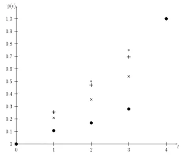
Consider now problem (3.29) with b = 4, A = 0, and B = 1. In Table 3.1 we show the extremal values ˜y(1), ˜y(2), ˜y(3), and corresponding ˜Jα, for some values of α. Our numerical

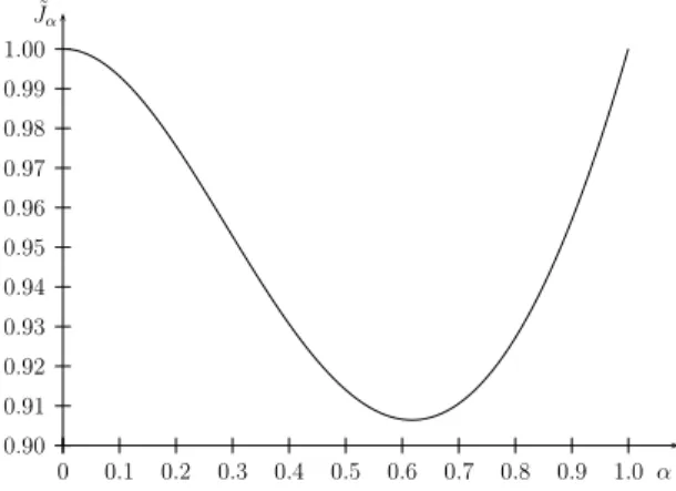
results show that the fractional extremal converges to the classical (integer order) extremal when α tends to one. This is illustrated in Figure 3.1. The numerical results from Table 3.1 and Figure 3.2 show that for this problem the smallest value of ˜Jα, α ∈]0, 1], occur for

α = 1 (i.e., the smallest value of ˜Jα occurs for the classical non-fractional case).

α y(1)˜ y(2)˜ y(3)˜ J˜α

0.25 0.10647146897355 0.16857982587479 0.2792657904952 0.90855653524095 0.50 0.20997375328084 0.35695538057743 0.54068241469816 0.67191601049869 0.75 0.25543605027861 0.4702345471038 0.69508876506414 0.4246209666969

1 0.25 0.5 0.75 0.25

Table 3.1: The extremal values ˜y(1), ˜y(2) and ˜y(3) of problem (3.29) with b = 4, A = 0, and B = 1 for different α’s.

Example 65. In this example we generalize problem (3.29) to Jα,β = b−1 ! t=0 γ1 ( 0∆αty(t) )2 + γ2 ( t∆β_by(t) )2

(51)

CHAPTER 3. _{FRACTIONAL VARIATIONAL PROBLEMS IN T}_{= Z} 0 0.1 0.2 0.3 0.4 0.5 0.6 0.7 0.8 0.9 1.0 0 1 2 3 4 × × × × × + + + + + * * * * * ˜ y(t) t

Figure 3.1: Extremal ˜y(t) of Example 64 with b = 4, A = 0, B = 1, and different α’s (_•: α = 0.25; ×: α = 0.5; +: α = 0.75; ∗: α = 1). 0 0.1 0.2 0.3 0.4 0.5 0.6 0.7 0.8 0.9 1.0 0 0.1 0.2 0.3 0.4 0.5 0.6 0.7 0.8 0.9 1.0 ˜ Jα α

Figure 3.2: Function ˜Jα of Example 64 with b = 4, A = 0, and B = 1.

Cálculo fraccional em escalas temporais

$%&'()*+*,-(.,

/-01,02*(3*45'4

89-:%-'(;2*::0'&*-(,<(=4:*-*4(>,<?'2*04

;2*:50'&*-(8*-:%-%4('&(>0<,(@:*-,4

Nuno Rafael de

Oliveira Bastos

Cálculo Fraccional em Escalas Temporais

Fractional Calculus on Time Scales

Contents

I

Synthesis

5

II

Original Work

21

Introduction

Part I

Synthesis

Chapter 1

Fractional Calculus

1.1

Discrete fractional calculus

1.2

Continuous fractional calculus

Chapter 2

Time Scales

2.1

Basic definitions

2.2

Calculus of Variations

Part II

Chapter 3

Fractional Variational Problems in

T

= Z

3.1

Introduction

3.2

Preliminaries

3.3

Main results

3.3.1

Fractional summation by parts

3.3.2

Necessary optimality conditions

3.4

Examples

**$%&'()+,-(.,**

**/-01,02(345'4**

**89-:%-'(;2::0'&-(,<(=4:-4(>,<?'2*04**

**;2:50'&-(8-:%-%4('&(>0<,(@:-,4**