COMPUTER-AIDED
DRUG DESIGN
Lead Discovery
João Rui Vieira Ribeiro
Tese de Doutoramento apresentada à
Faculdade de Ciências da Universidade do Porto Química
2014
C O MPU T ER -AI D ED D R U G D ESI G N - Le ad D isco ve ry João Rui V ieira RibeiroD
FCUP 2014 3.º CICLOD
D
D
!
COMPUTER-AIDED
DRUG DESIGN
Lead Discovery
João Rui Vieira Ribeiro
Programa Doutoral em Química Sustentável
Departamento de Química e Bioquímica 2014
Orientador
Maria João Ribeiro Nunes Ramos, Professor Catedrático, Faculdade de Ciências, Universidade do Porto
7
Acknowledgments
I would like to show my deepest gratitude to my supervisor, Professor Maria João Ramos, for the opportunity to develop this project and for giving me support, knowledge and guidance through these years. In the same spirit I would like to acknowledge Professor Pedro Fernandes for the solid support and advice, making each project move forward to the proper end.
I thank to Professor Klaus Shulten and John Stone from Theoretical and Computational Biophysics Group for receiving me for the 3 months work collaboration. I had the possibility to learn and develop my programming skills inside a high tech level environment only available in these kinds of groups. The experience was rewarding in the scientific level as well as in personal level.
I also thank to Nuno Cerqueira for the challenging work relationship that lead each software to a higher level of detail and functionality. Each brainstorm retrieved significant conclusions to be applied in each program. I also thank Irina for the practical guidance in our collaboration.
I would also like to thank to all members of the Theoretical and Computational Biochemistry Research Group that made my PhD student life pleasant. I have special gratitude to Zé, “Professora” Natércia, Daniel, Xana and Silvia for the patience shown in several episodes. I also thank Sérgio for the scientific discussions and advices. In the informatics universe I would like to thank to Oscar for not have blocked the entry of his office to me (I think I deserved it some times) and for the very instructive conversations. I would like to let my appreciation for the fellowship of Diana, Diogo, Gaspar, Marta, João Coimbra, Nini and those that I am inexcusable for not remember their names.
I cannot finish my acknowledgments without thank my parents for their support through all these years. Without you I would never get so far. And off course, I thank to Carla for the unconditional love and companionship given since we met.
This PhD had the financial support of FCT through the doctoral scholarship SFRH/BD/ 61324/2009.
8
10
Abstract
The present work focuses on the development of new bioinformatics tools to assist the user in a Computational Chemistry/Theoretical Chemistry laboratory, improving the Computer Aided Drug Design process. Often the use of already existing software requires a slow learning process, where simple tasks can reveal tricky to the non-expert users. As a consequence, interfaces were developed here too that make simple the task of the user.
An outline on Computer Aided Drug Design is given in the first chapter, highlighting the drug development cost and listing the subjects proposed to be developed and improved. In the second chapter, the theory behind the present work is described, focusing on the theory on which the pre-existing used software are based.
The remaining chapters refer to the developed work in these last four years, both already published and unpublished, being each chapter devoted to each developed software. The subjects covered in each chapter are: virtual screening and the developed software vsLab; chemical motifs inside protein structures and the software Chem-Path-Tracker; structural surfaces and volumes calculated by the software VolArea; and last the Computational Alanine Scanning Mutagenesis technique to study protein-protein interactions performed by the software CompASM.
All developed software are plug-ins of the world wide used molecular visualizer, Visual Molecular Dynamics (VMD). This association revealed very interesting and useful because it was possible to provide the software with the visual dimension, thus complementing the numerical results returned by the developed tools. In this way it is given to the user the possibility to inspect the results visually, which is crucial in most of the times to improve the quality of the conclusions to be retrieved.
12
Resumo
O trabalho presente nesta tese consiste no desenvolvimento de novas ferramentas bioinformáticas que visam auxiliar o utilizador num laboratório de Química Computacional/Química Teórica melhorando, assim, o processo de design de fármacos baseadas em estudos computacionais. A necessidade deste auxílio revela-se importante aquando da utilização de vários programas informáticos afetos a esta área. Por vezes a simples utilização de um programa informático exige uma curva de aprendizagem lenta, onde nem sempre a mais trivial operação é de fácil execução para os utilizadores mais inexperientes.
No primeiro capítulo é dada uma visão geral da temática do design de fármacos por meios computacionais, realçando a problemática dos custos associados a este tema, apresentando os pontos propostos a serem desenvolvidos e melhorados. No segundo capítulo é descrita a teoria que serve de base às ferramentas informáticas já existentes que foram utilizadas para o desenvolvimento deste trabalho.
Os restante capítulos são referentes ao trabalho desenvolvido no decorrer destes últimos quatro anos, publicados ou por publicar, sendo cada capítulo afeto a uma ferramenta informática. Os temas referentes a cada capítulo são: virtual screening e a ferramenta desenvolvida vsLab; padrões químicos contidos em estruturas proteicas e o programa
Chem-Path-Tracker; cálculo de superfícies e volumes de estruturas realizado pelo programa VolArea; e por último a técnica computacional de mutagénese por alaninas para o estudo de
interações proteína-proteína realizada pelo programa CompASM.
Todos os programas foram embutidos num programa de visualização molecular mundialmente utilizado denominado Visual Molecular Visualizer (VMD). Esta associação revelou-se bastante interessante e útil, pois foi possível dotar os programas da dimensão visual, complementando assim os resultados numéricos originados pelas ferramentas desenvolvidas. Assim é dada a possibilidade ao utilizador de inspecionar visualmente os resultados, muitas vezes crucial para melhorar a qualidade das conclusões a serem retiradas.
13
Résumé
Le présent travail se concentre sur le développement de nouveaux outils bioinformatiques pour aider l'utilisateur dans un laboratoire informatique Chimie / Chimie théorique, l'amélioration de la Assistée par Ordinateur processus Drug Design. Souvent, l'utilisation d'un logiciel déjà existant nécessite un processus d'apprentissage lent, où les tâches simples peuvent révéler difficile pour les utilisateurs non - experts. En conséquence, les interfaces ont été développés qui font ici aussi simple, la tâche de l'utilisateur.
Un aperçu sur Conception Assistée par Ordinateur drogue est donnée dans le premier chapitre, en soulignant le coût de développement de médicaments et la liste des sujets proposés pour être développé et amélioré. Dans le deuxième chapitre, la théorie derrière ce travail est décrit, en se concentrant sur la théorie sur laquelle sont basées les logiciels utilisés pré-existant.
Les chapitres se réfèrent au travail développé dans ces quatre dernières années, tous deux déjà publiés et non publiés, étant chaque chapitre consacré à chaque logiciel développé. Les sujets abordés dans chaque chapitre sont : le criblage virtuel et le vsLab logiciel développé ; motifs chimiques à l'intérieur des structures de protéines et le logiciel Chem -Path -Tracker , les surfaces et les volumes calculés par le VolArea logiciel structurelles et durent la technique informatique Alanine Scanning mutagenèse à étudier interactions protéine-protéine exécutées par le logiciel CompASM .
Tous les logiciels développés sont les plug-ins du monde de visualiseur large utilisé moléculaire, Visual Molecular Dynamics (VMD). Cette association a révélé très intéressant et utile, car il était possible de fournir le logiciel avec la dimension visuelle, complétant ainsi les résultats numériques retournées par les outils développés. De cette manière, il est donné à l'utilisateur la possibilité d'inspecter visuellement les résultats, ce qui est essentiel dans la plupart des fois d'améliorer la qualité des conclusions à récupérer.
15
Keywords
! 2C Two processing cores
! 4C Four processing cores
! ACD Available Chemical Directory
! ADT AutoDockTools
! AMDE/Tox Absorption, Metabolism, Excretion and
Toxicity
! ASM Alanine Scanning Mutagenesis
! AVG Average
! BDT Automatic Protein-Ligand Docking for
Everyone
! CADD Computer-Aided Drug Design
! CCC CUDA Compute Capability
! CMB Carbohydrate-Binding Modules
! CompASM Computational Alanine Scanning
Mutagenesis
! CPT Chem-Path-Tracker
! CUDA Compute Unified Device Architecture
! DFT Density Functional Theory
! FEP Free-Energy Perturbation
! FN False Negative
! FP False Positive
! GA Genetic Algorithm
! GPU Graphics Processing Units
! GUI Graphical user Interface
! HBonds Hydrogen Bonds
! HSPP Homology-derived Secondary Structure of
Proteins
! LGA Lamarckian Genetic Algorithm
! logP Partition Coefficient
! LS Local Search
! MADAMM Multi Staged Docking with anAautomated
Molecular Modeling
! MD Molecular Dynamics
! MM Molecular mechanics
! MMPBSA Molecular Mechanics/Poisson-Boltzmann
Surface Area
! NCI National Cancer Institute
16
! NSCA Non-Solvent Contact Area
! OSC Oxidosqualene Cyclase
! PDB Protein Data Bank
! PME Particle Mesh Ewald
! PT Points
! RESP Restrained ElectroStatic Potential
! RMSD Root Mean Square Deviation
! RNR Ribonucleotide Reductase
! SASA Solvent Accessible Surface Area
! SM Streaming Multiprocessor
! SP Streaming Processors
! TCL Tool Command Language
! TI Thermodynamics Integration
! TN True Negative
! TP True Positive
! vdW van der Walls
! VMD Visual Molecular Dynamics
17
Index
1.!
Introduction ... 22!
2.!
Methods ... 25!
2.1.!
Molecular Mechanics ... 25!
2.1.1.!
Introduction ... 25!
2.1.2.
!
The Force Field Energy ... 26!
2.1.2.1.
!
The Stretching Energy ... 27!
2.1.2.2.
!
The Bending Energy ... 28!
2.1.2.3.
!
The Torsional Energy ... 29!
2.1.2.4.
!
The Van Der Waals Energy ... 30!
2.1.2.5.
!
The Electrostatic Energy ... 32!
2.1.2.6.
!
The Force Field Parameterization ... 32!
2.1.3.
!
Molecular Dynamics ... 33!
2.1.3.1.
!
Simulation Time Step ... 34!
2.1.3.2.
!
Simulation Time Scale ... 34!
2.1.3.3.
!
Boundary Conditions ... 35!
2.1.4.
!
Predicting the Association Energy ... 35!
2.1.4.1.
!
Molecular Dynamics/Poisson-Boltzmann Surface Area ... 36!
2.1.5.
!
Molecular Docking ... 38!
2.1.5.1.
!
Search Algorithm ... 38!
2.1.5.2.
!
Scoring Function ... 39!
3.
!
Results and Discussion ... 41!
3.1.
!
Virtual Screening Lab (vsLab) ... 43!
3.1.1.
!
VsLab - An implementation for virtual high-throughput screening using AutoDock and VMD ... 45!
3.1.1.1.
!
Abstract ... 45!
3.1.1.2.
!
Introduction ... 45!
3.1.1.3.
!
AutoDock ... 47!
3.1.1.4.
!
Graphical User Interface ... 48!
3.1.1.5.
!
Conclusions ... 51!
3.2.
!
Chem-Path-Tracker ... 52!
3.2.1.
!
Chem-Path-Tracker - An automated tool to analyze chemical motifs in molecular structures. ... 54!
3.2.1.1.
!
Abstract ... 54!
3.2.1.2.
!
Introduction ... 54!
3.2.1.3.
!
Software Description ... 56!
18
3.2.1.3.2.
!
A modified Dijkstra’s algorithm ... 57!
3.2.1.3.3.
!
The output of Chem-Path-Tracker ... 60!
3.2.1.4.
!
Software Validation ... 62!
3.2.1.4.1.
!
Chemical motifs surrounding active sites ... 62!
3.2.1.4.2.
!
Guanine deaminase ... 63!
3.2.1.4.3.
!
Oxidosqualene cyclase ... 65!
3.2.1.4.4.
!
Identification of Cation-π interactions ... 67!
3.2.1.4.5.
!
Exploring Water Channels ... 68!
3.2.1.4.6.
!
Proton and electron transfers ... 71!
3.2.1.5.
!
Conclusions ... 74!
3.3.
!
VolArea ... 76!
3.3.1.
!
VolArea - A Bioinformatics tool to calculate the surface area and the volume of molecular systems ... 78!
3.3.1.1.
!
Abstract ... 78!
3.3.1.2.
!
Introduction ... 78!
3.3.1.3.
!
Methods ... 80!
3.3.1.3.1.
!
The Surface Area Algorithm ... 81!
3.3.1.3.2.
!
The Volume Algorithm ... 82!
3.3.1.4.
!
RESULTS AND DISCUSSION ... 86!
3.3.1.4.1.
!
Validation ... 86!
3.3.1.4.1.1.
!
Graphical Interface ... 89!
3.3.1.4.2.
!
Applications ... 91!
3.3.1.4.2.1.
!
Static structures assay ... 92!
3.3.1.4.2.2.
!
Multi-framed structures assay ... 94!
3.3.1.5.
!
Conclusion ... 96!
3.4.
!
VolArea and CUDA ... 98!
3.4.1.1.
!
Data Structure ... 100!
3.4.1.2.
!
Results ... 102!
3.4.1.3.
!
Conclusion ... 103!
3.5.
!
CompASM ... 104!
3.6.
!
CompASM - an Amber-VMD Alanine Scanning Mutagenesis plug-in. ... 106!
3.6.1.
!
Abstract ... 106!
3.6.2.!
Introduction ... 106!
3.6.3.!
Methodology ... 107!
3.6.4.!
Software Description ... 109!
3.6.5.!
Results ... 111!
3.6.6.!
Conclusions ... 115!
4.!
General Conclusions ... 116!
19
Index of figures
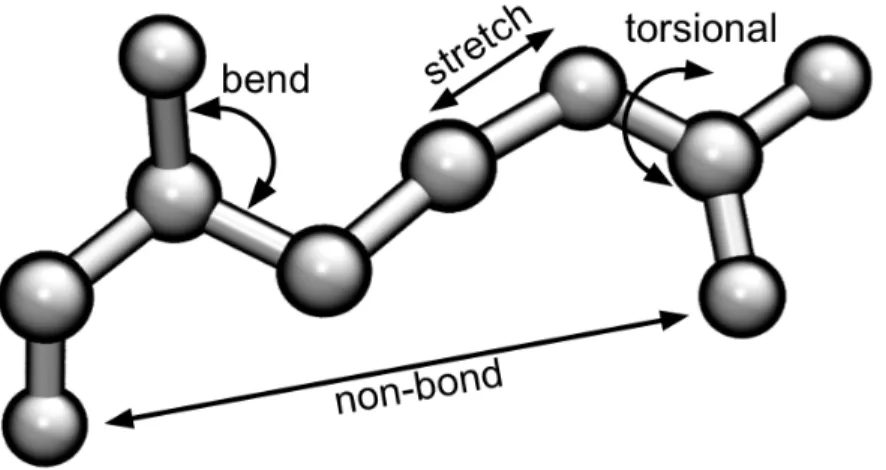
Figure 1- Terms of the Force Field Energy function. ... 26
!
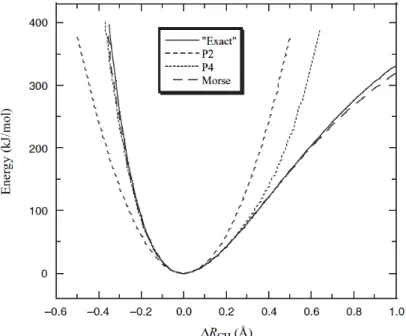
Figure 2- The stretching energy of the C-H bond of the CH4 molecule.. ... 28
!
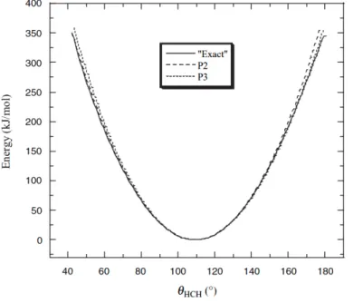
Figure 3- The bending energy of the H-C-H angle of the CH4 molecule.. ... 29
!
Figure 4- Illustration of the torsional angle definition. ... 30
!
Figure 5: Thermodynamic cycle used to calculate the binding free energy ... 36
!
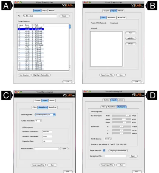
Figure 6: Graphical user interfaces available in vsLab ... 49
!
Figure 7: Sample VMD sessions displaying the results obtained from the vsLab plug-in. 50
!
Figure 8: Chem-Path-Tracker’s Graphical User Interface (GUI) input tab... ... 57!
Figure 9:!General algorithm implemented in Chem-Path-Tracker software. ... 60
!
Figure 10: Chem-Path-Tracker’s Graphical User Interface (GUI) output tab.. ... 61
!
Figure 11: Chemical interaction between the residues of the active site of the enzyme guanine deaminase that were highlighted by the Chem-Path-Tracker software.. ... 64
!
Figure 12: Most important chemical interactions present in the active site of OSC. ... 66
!
Figure 13: Graphical pathway that was highlighted by Chem-Path-Tracker revealing the (cation-π-)n stack chain found on the PDB structure with the code 3HHR. ... 68
!
Figure 14: Graphical pathway that was highlighted by Chem-Path-Tracker on the PDB structure with the code 2zz9. ... 70
!
Figure 15: Interaction network between the residues of monomer R2 of RNR provided by Chem-Path-Tracker (for the clarity of the image, Tryptophan 48 and 211 were not represented).. ... 72
!
Figure 16: Illustration of the usage of the probe radius to calculate the surface of molecules. ... 81
!
Figure 17: Schematic illustration of the searching radius superposition in order to illustrate the volume algorithm. ... 83
!
Figure 18: Example of the searching radius superposition, here applied to the cavity volume calculation. ... 84
!
Figure 19: Diagram of the algorithm that is used to calculate the volume in VolArea. ... 85
!
Figure 20: a) The relative error in the protein volume calculation (defined as the difference between the experimental and calculated volumes divided by the experimental volume) vs. the scale value and b) the average and standard deviation of the relative error for the 11 structures calculated.. ... 86
!
Figure 21: Variation of deviation as a function of the protein volume with a scale of 0.7 Å. ... 87
!
Figure 22: a) Average of the times of the protein volume calculation (using scale values from 1.0 to 0.7 Å) using four processing cores (4C) as a function of experimental volume, b)
20
ratio of the times in the volume calculation using two (2C) and four processing (4C) cores.
The speed up is linear. ... 88
!
Figure 23: VolArea Graphical interface:. ... 90
!
Figure 24: Surface values obtained with VolArea while analyzing the interface region of two proteins (retrieved from the PDB structure 1VFB):. ... 93
!
Figure 25: A) Exposed surface area of the residues located at the protein interface that interact more closely with the ligand.. ... 95
!
Figure 26: Simple representation of the NVIDIA Fermi GPU architecture. “A simplified hardware block diagram for the NVIDIA representing the arithmetic units “streaming processors” (SP) and “special function units” (SFU) for computing especial algebraic functions ... 99
!
Figure 27: Schematization of the organization of the atoms in bins ... 101
!
Figure 28: Chart displaying the gains retrieved from GPU.. ... 102
!
Figure 29: General algorithm of the CompASM procedure 27. ... 108
!
Figure 30:Scheme representing the Non-Solvent Contact Area (NSCA) ... 110
!
Figure 31: Results of the protein-protein interface study of immunoglobulin complexed with an egg lysozyme (detailed results in supporting information). ... 111
!
21
Index of Tables
Table I - Summary of the software’s available for calculating the volume and the surface of structures. ... 80
!
Table II - Results originated by CompASM. The Non-Solvent Contacting Area (NSCA) is calculated by the CompASM program. ... 113
!
Table III - Comparison of the values obtained using CompASM with those that result from the software/servers available. ... 114
!
22
1. Introduction
The discovery of new therapeutic compounds and the improvement of existing drugs are crucial aspects for every modern society, especially for rational drug design where the time and the costs of the process must be controlled and environmental harmless procedures
must be taken. Despite some divergences in terms of the real cost of drug design1-4, some
authors suggested that it is necessary more than 8 years and millions of dollars (between 800 and 2000 million US dollars) to develop a new therapeutic compound. These predictions are based in the probability of the new drug successfully pass each clinical trial phase. Here, the primordial steps of the drug design are extremely important to improve these probabilities, mainly when computational means are efficiently used.
Independently of the chosen methodology to develop a new drug, crucial steps are required, such as the identification of hit compounds and improvement of the lead compounds; the correct study and description of the drug target, and the prediction of the effects of the drug in terms of absorption, metabolism, excretion and toxicity (AMDE/Tox). Despite the possibility of performing these steps in vitro, it is using computational tools where major gains are obtained.
Computer-Aided Drug Design (CADD) is a field of research that comprehends a vast collection of computational solutions to store, manage, analyze and model chemical compounds. Here, the main purpose is to simulate ligand-receptor complexes in biological conditions in order to predict chemical properties to anticipate and manipulate drugs functionality and behavior. One of the greatest advantages of a CADD campaign is the possibility to select or model the potential compounds; calculate the drug-receptor binding properties and optimize compounds in silico, avoiding the usage and production of harmful substances. Only then, the most promising compounds are experimentally synthetized and tested improving the success and speed, i.e. reducing the costs of drug discovery.
The bases of the new potential drug commonly derive from one or more databases
containing a massive number of molecules, which is the case of the ZINC database 5
(despite the name it is not a Zinc based compound database). This free repository in particular contains about 21 million compounds prepared for virtual screening in their biologically relevant forms. Besides the atoms’ 3D-coordinates, this database contains the values that describe the residues protonation states, molecular weights, calculated LogP and the rotatable bonds, making ZINC database an important source for CADD campaigns. Beside this repository, there are many other repositories containing a large number of structures as well, which is the case of Available Chemical Directory (ACD, over 7 million
23
compounds)7 among others 8-10, in which some of them unfortunately are not so completed in
terms of biological significant values.
One keystone of the drug design process is the full characterization of the target structure, even before the selection of the possible candidates from the previous mentioned databases. Generally, these structures are obtained from experimental means and stored in the Protein
Data Bank (PDB) 11,12. This database is composed by the structures of large biological
molecules, such as proteins and nucleic acids, mainly resolved by X-Ray Crystallography/Diffraction and Nuclear Magnetic Resonance (NMR). However, when the experimental 3D-structure is not available, the most reliable technique to use is Homology
Modelling 13-15 or to extract the structure from the homology based, Homology-derived
Secondary Structure of Proteins(HSPP) database 16,17.
The availability of such amount of information is a vital aspect for computational chemists allowing the application of CADD techniques in a wide variety of biological processes, using
appropriate and successfully proven methodologies such as molecular docking18 and virtual
screening19. CADD methodologies have been supported by the appearance of numerous
scientific software focused on drug design or molecular simulations, serving different
purposes, presenting more or less accurate results, freely available or purchasable 20-24. The
development of efficient parallel algorithms has boosted CADD even further, and lately the
usage of Graphics Processing Units (GPU) in massive parallel operations 25 has resulted in
significant gains in terms of speed and allowed size of the simulated systems. On the other hand, large collections of structures and software specialization can also bring difficulties and challenges to the researcher in his/her projects. Here, bioinformatics play an important role creating tools to complement existing software, turning all this information usable and manageable. Using these tools is possible to extract significant and relevant values, improving in this way the efficiency of CADD campaigns.
Examples of such demand for process optimization in CADD methods is felt, for instance, when it is necessary to evaluate the binding of a large set of compounds extracted from one of the previously mentioned databases. It is thus necessary to analyze the poses of those structures against the target’s binding site and rank the ligands regarding the strength of binding interactions or other parameters. The information required to perform this process would be impossible to handle manually, and even computationally users would have to be familiar with programming languages such as Python or Tool Command Language (TCL). For instance, at the end of a protein-ligand docking calculation, the total number of files originated by the software can easily double or quadruple the number of structures files (e.g.
using Autodock26), making the extraction of the information of interest laborious and
hardworking. The same exponential growth of generated information can occur when another CADD technique is applied, namely Computational Alanine Scanning Mutagenesis
24
(CompASM)27. This method analyzes protein-protein interfaces, identifying the residues that
contribute more for the binding of the intervening systems. CompASM is based on the premise that residues responsible for the binding of the proteins (hotspots) cause significant
variations in the binding energy of the complex when mutated by an alanine residue28.
Moreira et al. proposed a successful protocol for a computational application of ASM which comprehends Molecular Dynamics (MD) simulations and Molecular
Mechanics/Poisson-Boltzmann Surface Area (MMPBSA)29 calculations.
Despite the major improvements in protein-ligand docking, virtual screening and ASM methods, several developments are required in order to bring this analysis to general use and to non-expert users. These new tools must have the ability to assist the user in the generation and parameterization of the input data and assemble the final results, displaying them in a user-friendly manner.
The work presented in this thesis provides solutions to assist computational chemists in their daily work, developing new tools to simplify the application of Molecular Docking, Virtual Screening, and Computational Alanine Scanning Mutagenesis, applying world-wide used
software such as AutoDock26, and the Amber molecular simulation package30. In this chapter
new algorithms are described to calculate protein structural features, namely surface residues in contact with solvent or other compounds, as well as to calculate the volume of any structure and empty spaces such as cavities and clefts. It is also presented a bioinformatics tool to identify and track chemical motifs (hydrogen bonds, cation-π-interactions, proton-electron transfer pathways and water tunnels) throughout a protein/molecular system. In order to provide a visual aspect to the user, allowing the inspection of the results, the developed tools are compatible with the widely used molecular
25
2. Methods
This section intends to give an overview of the theoretical methods applied in the developed work, in order to provide the foundations of the software used in the presenting new bioinformatics tools. The covered subjects are: Molecular Mechanics, Molecular Dynamics highlighting the specific binding energy calculation method Molecular Mechanics/Poisson-Boltzmann Surface Area (MMPBSA); and Molecular Docking, in particular Protein-Ligand Docking and Virtual Screening. In each topic, the theoretical contents associated to each subject is described numbering the most used software. A full
method description and deeper understanding of computational chemistry is presented in 32.
2.1. Molecular Mechanics
2.1.1. Introduction
Molecular mechanics (MM) is a simplification of the molecular structure model to an aggregated complex of “balls and springs”, where the unitary particle is the atom, neglecting electrons and protons as individual particles. In MM methods, the information assigned to each particle (atom) is the atomic mass, charge, van der Waals radii and instead of calculating the bonding information as a product of the Schrödinger equation, the values for bond lengths, bond angles and dihedral angles are provided explicitly as parameters of the
force field. Since the first published paper applying molecular mechanics calculations33,
several works have been published using this method with very interesting and promising
results27,34-38. The application of this method to biomolecules has got great acceptance
mainly because of the relative good performances in terms of speed and final results. Other important factor that contributed to the generalization usage of these methods were the increase of the community users that have applied these tools through these last decades, making somewhat easy to obtain the parameters for a wide range of structures type. At the same time, the requirement for these parameters is one of the drawbacks of this methodology, which are not always available, requiring its calculation. This method also fails when a deeper understanding of the system is intended, for instance, the study of formation and breaking of the chemical bonds.
In spite of the negative aspects, MM methods are still a very powerful strategy for molecular simulations and drug design. For instance, it is now possible to simulate 1 million atoms model of the satellite tobacco mosaic virus with a simulated time of 50 nanoseconds (ns) 39. The application of these methodologies is quite straightforward while the type of
26
atoms in the system remains common or is possible to obtain the parameters from other user
calculations. In both cases, MM packages such AMBER40, CHARMM41, GROMACS42
incorporate a large source of parameters for a wide range of biological molecules, such as amino acids and nucleotides, and have a large community of users. This last factor increases the probabilities of finding some missing parameters, allowing the simulation of a wide range types of systems.
2.1.2. The Force Field Energy
Molecular Mechanics describes the force field energy (!!!) as the sum of the terms
describing the energy required to distort a molecule in a specific way:
This equation is composed by energy functions that deal with bond interactions,
non-bound interactions and cross-terms, being the first three terms the stretching energy (!!"#),
the bending energy (!!"#$) and the torsional energy (!!"#) functions to describe the
interactions between bonded atoms; the following two are the van der Waals (!!"#) and
electrostatic energy (!!"!) functions to describe the unbound interactions, and the last term of
the equation is the combination of the any of the previous terms.
Figure 1- Terms of the Force Field Energy function.
The differences in the composition and complexity of the equations adopted to calculate these energies are mainly determined by the problem to be solved by the different force fields. For instance, the AMBER force field aims at dealing with biological systems, which can easily turn very computationally demanding due to the size of the complexes. In this
27
case simplified functions are required, describing only the bond and non-bond terms, dismissing the description of the out-of-the-plane bending energy and the cross-term. All molecular simulations presented in this work were carried out using the AMBER force field, and only the terms contained in this force field will be described in the following sections.
2.1.2.1.
The Stretching Energy
!!"# is the function of the energy associated to the elongation of the bond between two atoms (A and B) around the equilibrium bond length. A simple way to calculate this value is by the harmonic potential presented in equation (2).
In equation (2) !!" defines the bond force constant and !
!!" defines the equilibrium
bond length between atoms A and B. Despite the good results obtained by this potential in equilibrium geometries, a more accurate solution is required to analyze long-range bond distance or when it is necessary to include additional energy terms such as vibration energies.
The Taylor expansion of the harmonic potential up to the fourth term in equation (3) is a better energy descriptor when it is necessary to analyze these energies beyond the equilibrium bond length.
In spite of the better result, this expansion still presents two major drawbacks: the first one is the requirement of more parameters to be assigned, and the second one is the tendency to infinity (+∞) in long bond lengths, instead of a tendency to a constant energy, the dissociation energy.
The most accurate method to calculate the stretching energy is through the Morse potential (4), unfortunately this method is also the most slow/computationally demanding method. !!"# !!" = !!" !!"− !!!!" != ! !!" ∆!!" !! (2) !!"# !!" = !!!" ∆!!" !+ !!!!" ∆!!" !+ !!!!" ∆!!" !! (3) !!"#$% ∆! = !(1 − !!!∆!)!! ! = ! 2!! (4)
28
Like the previous potential, this method also requires some parameters such as the dissociation energy ! and the force constant at the equilibrium distance !.
Figure 2- The stretching energy of the C-H bond of the CH4 molecule. The exact curve was based on an electronic structure calculation with CASSCF/6-311++G(2df,2dp), the P2 and P4 curve stands for the simple harmonic potential and the Taylor Expansion of the harmonic potential, respectively 32.
At ambient or biological temperature, the bond length usually presents a variation of 0.03Å and the curve region of interest for simulation purposes is the bottom energy ~40 kJ/mol. In this region, all methods present close results, differing only in the computational and parameters requirements. In this case, the simple harmonic potential does not introduce significant errors, being profitable mainly by the calculation speed. The force field used in this work, AMBER force field, implemented the harmonic potential as the elected method to calculate stretching energies.
2.1.2.2.
The Bending Energy
The !!"#$ energy function describes the energy necessary to change the angle formed by
three atoms A-B-C, centered on atom B. Just like in the previous term, the bending energy is efficiently described by the simple harmonic potential (5). This potential formulation also
requires the parameterization of the force constant !!"# and instead of the equilibrium bond
length !!!", here it is required the value of the equilibrium bond angle !!!"#.
!!"# !!"# = !!"# !!"#− !!
29
If a more accurate solution is required, the third term of the Taylor expansion returns a reasonable value, which is not normally necessary as it is possible to see in Figure 3.
Figure 3- The bending energy of the H-C-H angle of the CH4 molecule. The exact curve was based on an electronic structure calculation with (MP2/aug-cc-pVTZ), the P2 and P3 curve stands for the simple harmonic potential and the Taylor Expansion of the harmonic potential, respectively 32.
As mentioned previously, at the bottom 40 kJ/mol energy of the curve (equivalent to most hydrogen bond energies), both methods fit reasonably well to the energy curve, being the simple harmonic potential more efficiently computed mainly due to the requirement of only two parameters.
2.1.2.3.
The Torsional Energy
!!"# (torsional energy) is the energy necessary to rotate atoms A or D around bond B-C in
30
Figure 4- Illustration of the torsional angle definition.
Unlike the !!"# and !!"#$ functions, the harmonic potential is not the perfect solution to
calculate the torsional energy mainly by the absence of descriptors for two observed behaviors in this type of distortion: one is the periodic movements allowed when the atoms are rotated in turn of the central bond, and the other is the low energy requirement to alternate between different minima.
To incorporate the missing aspects, a Fourier series (6) is used instead of the harmonic potential.
The periodicity of this function is acquired by the ! term, which provides to each period nth
rotation angles: ! = 1 term describes a 360º periodicity, ! = 2 describes a period in each
180º, ! = 3 term determines periodicity in each 120º, and so on. The !! constant is the size
of the barrier of the rotation around the B-C bond. The ! factor, the division by 2 and the summation of 1 are operations necessary to produce standard outputs so the values
returned by this equation may have a user defined minimum at 180º, and the !!"#/ !! values
vary between one and zero.
2.1.2.4.
The Van Der Waals Energy
The van der Waals (E!"#) energy function term is the first descriptor for the non-bonded
atoms interactions. This term is correlated with the non-polar interaction between the atoms, describing the attraction and repulsion provoked by the electron clouds surrounding the nuclei. This physical property explains the energy variation, in which at very small distances,
!!"# !!"#$ = ! !!!
!!!"#$
31
the E!"# energy becomes positive, reflecting the repulsion forced by the overlap of the electron clouds. At median distances, about 3.5 Å, this energy becomes slightly negative (attractive) due to the induced dipole-dipole forces, tending to zero at very long distances, a
R-6 dependency, being R the distances between the two atoms.
The Lennard-Jones potential (7) reflects the behavior described above, presenting
two parameters, the van der Waals radius !! and the softness factor (!).
The 12 exponential factor of the repulsive fraction of the equation is not related with physical evidences or theoretical basis, in which the values 9 or 10 returned better results. The usage of this factor is only associated with computational intrinsic features, which are calculated by squaring the attractive fraction with the exponential factor 6.
If a better descriptor is required, it is possible to calculate this energy using two
different potentials: on is the “Buckingham” or “Exponential R-6” potential (8), and the other
one is the Morse potential. In the first potential, A B and C factors are constants and the !!"
is the distance between the atom A and B.
Despite the better accuracy of this potential, its usage can also constitute a source of
error, especially at very small distances, where the (!!")!! tends to −∞ creating a “nuclear
fusion”, instead of becoming a positive repulsive energy. The Morse potential increases the accuracy of the results in all circumstances, but it also increases the computational time necessary to calculate these interactions like explained before.
The non-bonded atom interactions require special attention in terms of the computational time requirements. This problem becomes even more important in biological systems, since they contain a large number of atoms. While the number of bonded interactions increase linearly with the number of the atoms, the non-bonded interactions grow as the square of the system’s size, turning the calculations of these energies the predominant procedure in the force field energy calculation.
To reduce the calculation time of the non-bonded energies, one or more cut-off distances can be applied. In the case of one cut-off distance, in which the van der Waals energy becomes zero at great distances, the potential becomes a discontinuous descriptor. To solve this problem, a two cut-off distance approach can be adopted, in which a smothering function is applied between the two distances values, where the energy slowly tends to zero between these two energies.
!!" !!" = !4! !!!" !!" !" − ! !! !" !!" ! ! (7) !!"# !!" = !!!!!!"− ! ! (!!")!! (8)
32
2.1.2.5.
The Electrostatic Energy
The electrostatic energy (E!"!) term of the force field energy equation is the second
non-bond interaction descriptor. This term describes the electrostatic interactions between the average point charges of the atoms in the system and it is calculated based on the Coulomb potential (9).
In this potential, !! and !! are the charges of the correspondent atoms A and B, !!" is
the distance between them and ! is the dielectric constant of the medium. The dielectric ! can be parameterized to simulate the electronic environment of the system, such as ! = 1 for vacuum, or higher values; for instance ! = 4 for proteins and ! = 80 for water, simulating the water as the solvent in the absence of explicit water molecules.
In a physical sense, the atom point charge is not fully correct, being adopted as the point that describes better the arrangement of the electric field around the atom. This concept is applied in the AMBER force field through the Restrained ElectroStatic Potential fit (RESP).
The E!"! energy describes not only the influence of the formal charged atoms in the system, just like the oxygen atom in a hydroxide molecule, but also the partial charged atoms. Here, dipole-dipole interactions and hydrogen bonds are also implicitly included. For instance, an alcohol oxygen atom partially negatively charged would have the tendency to interact favorably with a partially positively charged hydrogen atom from another alcohol group. One of the most severe limitations of molecular mechanics is related to this function, in which the surrounding atom environment has no influence in the point charges of the atoms, keeping their charges static through the simulation calculation.
2.1.2.6.
The Force Field Parameterization
Besides the importance of the equations choice to describe the different terms of the force field, the efficient and accurate parameterization of the constants in the equation also plays a central role in the molecular mechanics methods. In spite of no force field parameterization having been performed in this work, this subject has a relevant importance in molecular simulations.
For an ordinary structure such as proteins, most of the parameters are included in the molecular simulations packages. However, this is not the case for most substrates or inhibitors, in which the calculation of parameters like the stretching energy constant force K!", or the torsional barrier size, is required. This last term is problematic due to the number
of possibilities.
!!"! !!" = !
!!!!
33
There are two ways for a computational chemist to obtain values for these parameters: one is deriving them from experimental values, but we are always conditioned by their availability, and the other option is by computational means, which are relatively easier, cheaper and straightforward to apply. Here, sophisticated computational methods such as Density Functional Theory (DFT) or post Hartree-Fock methods can be applied. In the case of the stretching energy, the parameters can be obtained by structure optimization and posterior scan, where the bond length is stretched and shrunken until the equilibrium value is reached. Later, this data is fitted to the harmonic potential or other potential.
The van der Waals parameters are normally assigned to single atoms directly from the experimental data, and later combined for the diatomic value. The simplest approach is to calculate the diatomic van der Waals distance as the sum of the two van der Waals radii, and the softness factor as the geometrical mean of the atomic softness constants.
As mentioned above, the charge parameter should describe the electrostatic field surrounding the atom, instead of a group of single point charges. These charges are calculated by the electrostatic potential of a series of points in a grid around the desired molecule, and adapted later to single points that reproduce better those values.
2.1.3. Molecular Dynamics
One of the most relevant applications of the molecular mechanics principles is in the description of the trajectories of the atomic structures throughout time. Here, Molecular Dynamics (MD) simulations describe the atoms’ Cartesian coordinates that have suffered the influences of the other atoms. The movements of the atoms are simulated by solving Newton’s second equation, ! = !", in order to obtain a time dependent descriptor (10).
The previous equation describes the trajectory of particle ! with mass !! along one
coordinate !! with !!! representing the force acting on the particle in that particular direction.
This force is calculated based on the potential energy obtained from the terms described in the earlier sections. This mobility description is deterministic, meaning that for any value of time variable, the state of the system can be calculated once the position and the velocities are deduced.
In Molecular simulations, this function is applied by the Newton’s equation as a function of 3N coordinates (i.e. the 3D spatial location). The complexity of the systems usually analyzed by this function turns the analytical solution impossible, requiring therefore the numerical
!!! ! !"! = ! − !!! !!! (10)
34
resolution of the equations. To do so is necessary to define a finite integration step denominated simulation time step (!").
2.1.3.1.
Simulation Time Step
The proper parameterization of the integration step requires special care that will determine the right description of molecular behavior. This time step must be set as a function of the quickest motion period to be described, and at the same time, the value that returns a relative economy in terms of computational demand and time consumption. The wrong parameterization of this value can lead to a mismatched description of the atoms trajectories due to the abrupt variation of the potential energy, or a software breakdown due to the numerical overflow.
The common rule applied to choose this value is the calculation of the number that is at least one order of magnitude smaller compared to the highest-frequency vibration motion in biological structures. This motion is the bond stretching movement involving hydrogen atoms, which is around 10 fs (e.g. the C-H bond stretching), originating an integration step of 1 fs. Despite of the fact that C-H bond stretching is the fastest motion period, its influence in terms of the potential energy variation is not significant, and the respective fluctuations do not imprint a significant numerical instability, giving space to restrain their variation and therefore
save computational time. To perform these constrains, the SHAKE algorithm 43 is usually
applied, in which the bonds containing hydrogen atoms are frozen to their equilibrium values, and the highest-frequency vibrations in the system are now the bonds stretching between heavy atoms such as the C-C bond. These frequencies have a motion period between 2 and 5 times slower (20 to 50 fs) than the hydrogen intervenient bonds, which is translated in a suggested time step of 2 fs.
2.1.3.2.
Simulation Time Scale
Besides the integration step, there is another time variable, which is the time simulation. This time scale defines the time range in which the atoms trajectories will be simulated. The value of this variable is related to the kind of structural motions that is intended to observe. For instance, if only the atoms position fluctuations or side chains motions are intended to simulate, the time range necessary to observe these variations is in the order of picoseconds. On the other hand, loop motions can take several nanoseconds, a protein subunit motion or even the folding and unfolding of protein could be out of the scope of this method. The choice of these values can also be influenced by the size of the system. Here, the total cost in terms of computational time can be very high. The values of time scale that
35
establish a good commitment between the computational time (real time) and the quality of the simulated trajectory are in the range of the hundreds of nanoseconds for the enzymatic systems.
2.1.3.3.
Boundary Conditions
In biological environment, it is possible to admit that a molecule is immersed in infinite universe, or has infinite space around it in all directions. In a molecular dynamics simulation
containing explicit solvent water molecules (e.g. TIP3P44) instead of an implicit description of
the solvent, is necessary to define the simulated space. In this work, this option was not applied, but like the force field parameterization, boundary conditions are also very important in the molecular dynamics simulations field.
As mentioned beforehand, the size of a molecular structure, for instance, a protein, compared to the intracellular space is substantially small, considering that there is infinite space surrounding a protein in a biological environment. Being computationally impossible to simulate an infinite space, a set of cut-off distances defining the borders of the system must be applied. Here, a box containing the structure and the solvent molecules must be defined. The edges of the simulation box are described as the edges of the copies of simulation box. These copies placed around the simulation box are in contact with each other in a way that, for instance, a solvent molecule describing a trajectory that goes out of the bottom of the simulation box, will appear on the top of this same box.
The size of the simulation box must be defined carefully in order to avoid self-interaction (the interaction between a molecule located in a boundary limit and itself). As mentioned in
the E!"! section, a set of cut-off distances must be used, and a special method to deal with
these interactions is through the application of the Particle Mesh Ewald (PME)45.
2.1.4. Predicting the Association Energy
One of the most important values to be determined in this kind of simulation is the Gibbs free energy of association. The importance of these values is revealed in several computational studies, such as the evaluation of the binding of a protein with small ligands
(e.g. enzyme-ligand binding), or the binding between larger structures like two proteins 46-49.
It is in the former subject that this free energy prediction took relevant weight in this work.
Here, the method used to calculated the Gibbs free energy (!! ) was the Molecular
Mechanics/Poisson-Boltzmann Surface Area (MMPBSA)50 implemented in the molecular
simulation package AMBER30. More accurate methods could be used for the same purposes,
36
methods, which in fact return better results. The reason for the choice of the MMPBSA method in detriment of FEP and TI is the higher computational efficiency of the MMPBSA. For protein-protein association analyses, MMPBSA presents relatively good agreement to the experimental results without compromising the computational time required. Only the MMPBSA method will be described in the following section because it was the only free energy calculation method used in this work.
2.1.4.1.
Molecular Dynamics/Poisson-Boltzmann Surface Area
The values of free energies calculated through molecular mechanics methods are not accurate enough to perform, for instance, a comparison between different systems. This feature relies in intrinsic properties of the MM method where the zero point of the energies descriptors must be parameterized, which in most cases is not the same for all force fields and the approximations necessary to solve the equations mentioned beforehand also induce a certain level of errors. This error accumulation leads to significant differences in the final value, making it devoid of scientific meaning. Instead of considering only one final free energy value, the binding free energy values can be compared based on error cancelation, retrieving a variation on the binding free energy, which is provided of scientific accuracy. In this work, these values are used for the analysis of the variation of the binding free energy of the system when a residue on a protein-protein surface is mutated by an alanine. The resulting Alanine Scanning Mutagenesis Method is described in the results section.
The MMPBSA methodology conjugates a molecular mechanics energy calculation with a molecular dynamics simulation in implicit solvent. The binding free energy can be calculated
using the thermodynamic cycle shown in Figure 5, in which ∆Ggas is the interaction free
energy between the two binding partners in the gas phase, and ∆!!"#$!"# ,
∆!!"#$!"#"$!"#!∆!!"#$!!"#$%&!are the solvation free energies of the two binding partners and the complex, respectively.
37
The binding free energy of two molecules in a complex is defined as the difference between the free energy of the complex and the respective monomers (11).
The free energy of the complex and the respective monomers can be calculated by
summing the internal energy (bond stretching, angle bending, and torsional energy), Einternal;
the electrostatic and the van der Waals interactions, Eelectrostatic and EvdW; the free energy of
polar solvation, Gpolar solvation; the free energy of nonpolar solvation, Gnonpolar solvation; and the
entropic TS contribution for the molecule’s free energy as is written in equation (12).
The first three terms are retrieved from the force field applied in the molecular dynamics simulation. The electrostatic solvation free energy can be calculated by solving the
Poisson−Boltzmann equation with the Delphi software51-53, which has been shown to
constitute a good compromise between accuracy and computing time. During the Poisson-Boltzmann equation solving process, two different dielectric constants are assigned in order to simulate two different environments: one refers to the external/solvent medium which is normally assigned with the value 80 (! = 80) for water solvent medium or ! = 1 in case of vacuum, and 2! < !! < 4 in the case of the solute/protein environment.
The nonpolar contribution to solvation free energy by the van der Waals interactions between the solute and the solvent, and cavity formation, is modeled as a term dependent on the solvent-accessible surface area of the molecule. It is estimated using the empirical relation,
where A is the solvent-accessible surface area calculated by the molsurf program, which is based on the idea primarily developed by Michael Connolly 54 and it is implemented in the
AMBER molecular package. α and β are empirical constants, with values 0.005%42 kcal Å
-2 mol-1 and 0.92 kcal mol-1, respectively. The entropy term, obtained as the sum of the
translational, rotational, and vibrational components, will not be calculated because it is assumed, on the basis of previous work, that its contribution to the ΔΔGbinding is negligible55,56.
∆!!"#$"#%!!"#$%&#$= !!"#$%&'− !(!"#$%&!!"#"$%&'! (11)
!!"#$%&#$= !!"#$%"&'+ !!"!#$%&'$($)#+ !!"#+ !!"#$%!!"#$%&'"(+
!!"!#"$%&!!"#$%&'"(− !" !
(12)
38
2.1.5. Molecular Docking
Molecular Docking is one of the most used molecular modeling methods in computer-aided drug design. This method is usually the first approach in the drug discovery process when the receptor structure is known, often extracted from the Protein Data Bank (PDB)
11,12or similar database. Instead of just characterizing the position and orientation of one
ligand inside the receptor binding site (docking campaign), this method reflects its full benefits in the characterization and sorting of several ligands (virtual screening). The main goal of virtual screening campaigns is to select the compounds that have higher probabilities to develop a strong binding (e.g. inhibitor or substrate) and ranking them by their docking score and/or predicted binding energy.
Molecular docking software are characterized by their search algorithm, sometimes named optimization algorithm, and their scoring function. The differences in the search algorithms are related to the model and the allowed degrees of freedom in the ligand and receptor structures. Looking at the scoring functions, some software adopts molecular mechanics model approximations like in the force field energy calculation, or empirical or knowledge-based scoring functions. The combination and tuning of the search algorithm and scoring function is always dependent of the accuracy/computational demand relationship that dictates the general usage of the program, especially in databases containing a vast number of compounds.
There are good reviews in the literature concerning molecular docking, e.g. the reviews from Sousa et. al 18,57.
2.1.5.1.
Search Algorithm
The simplest search algorithm to be considered is an algorithm that treats all the complex units as rigid bodies and only the rotation and translation of the units around each other are considered. This type of algorithms can be very useful in virtual screening campaigns, in which a large amount of ligands are evaluated. The speed of this kind of methods allows the analyses of large databases of small ligands, and suits even better in the docking of large structures as is the case of protein-protein docking58. On the other hand, the molecular
description is not enough in the cases where some conformational changes have to take
place in order to allow a proper interaction between the ligand and the receptor59. In these
cases some flexibility (or even the full flexibility) of the complex is required and is implemented in the search algorithms of the docking software through three different methods: systematic, random or stochastic and simulations methods.
39
In the systematic methods category, the conformational search, fragment-based and database-based algorithms are included. The conformational search algorithm is based on the analysis of all possible conformations originated by the rotation of the dihedral angles of the ligand. In case of the fragment-based, the algorithm tries to bind small parts of the ligand, adding groups to the initial structure until the full structure is completely docked in the receptor binding site. Regarding the database-based method, this algorithm is based on the docking of rigid structures. The ligand structures are generated computationally or experimentally and only the structures that present higher probability to exist are considered.
Random or stochastic methods are the most applied search algorithms in docking software. An example of a random algorithm is the Genetic Algorithm (GA) implemented in
AutoDock or Gold60,61, where the search routine is based in the Darwin survival theory and
the Mendel genetics processes like mutations and genes transmission. Another algorithm often implemented in docking programs is the Monte Carlo algorithm, which is very useful when it is intended to evaluate a wide range of conformations, such as the Tabu algorithm. In this algorithm several structures are generated avoiding the creation of equal structures, giving also a wide variety of structures.
The simulation search methods apply molecular dynamics simulations and/or energy minimization calculations. These methods are suitable for the optimization of the structures resulted from a previous virtual screening or docking campaign. The convergence rate of these algorithms is low and very computational demanding.
Published works like MADAMM (multi staged docking with an automated molecular
modeling protocol), from Cerqueira et al.38, apply a combination of systematic algorithms and
simulation methods, with a rigid body docking in order to improve the docking results. The major drawback of these protocols is the time required to evaluate all the conformations and the molecular simulations, which despite of improvements, are still considerably slow for a general application in a large database.
2.1.5.2.
Scoring Function
Searching for the best conformation of a ligand-receptor binding complex could not be complete if the evaluation of these conformations took place. Actually, the evaluation (scoring) and the search routines are intercalated in the docking process. For instance, in the Genetic Algorithm, the elements of the genes can only be transmitted to the next generations if they are fit to survive.
As with the search algorithms, different software apply different methods to evaluate the binding of the ligand into the receptor binding site, namely: force field, empirical, knowledge-based, and consensus scoring functions. The force field scoring functions are based on the
40
numerical calculation of the energy applied in the molecular energy descriptors described in the 2.1.2 section, just like internal energy calculation (bond stretching, angle bending and torsional energy). As mentioned beforehand, as the molecular descriptor becomes more sophisticated, the computational demand becomes an issue, turning the application of this kind of scoring functions not practical for fast docking processes.
The empirical scoring functions are based on experimental observations, in which it is intended to recreate these values by approximated and parameterized functions. Despite the speed of calculation of these functions, these parameters are not transferable to all structures, demanding constant parameterization, function tuning and constant search for experimental values (which are not availability for all cases). Knowledge-based functions employ the same parameters approximation, but instead of an energy calculation, these functions are focused on geometry optimization.
Instead of being a different method to score docked conformations, the consensus functions are the combination of the previously mentioned scoring functions. This approach is based on error cancelation while maintaining the advantages of the features of each method.
41
3. Results and Discussion
This chapter intends to report the accomplished work, either published or to be published, describing the resultant software. The descriptions of the new bioinformatics tools are based on the correspondent scientific papers, complemented with relevant information regarding, the software used to perform molecular calculations, theoretical information or developments carried out since their release. The visual inspection of the structures and the results is obtained by the inclusion of all developed tools in the world wide web molecular visualizer, Visual Molecular Dynamics (VMD).
The first section of this chapter describes the software vsLab, which was developed to assist the user in virtual screening campaigns and is based on one of the most used molecular docking software, AutoDock. This program allows the user to perform a virtual screening campaign in a very easy-to-use fashion. All the parameters required to carry a molecular docking prediction are set in a Graphical User Interface (GUI) in which the resultant ranking of the docked ligands is displayed, sorted by the docking score returned by the AutoDock software. The code under the GUI manages all the files necessary to launch the AutoDock calculations and also deals with all intermediate steps of the molecular docking protocol, including the structure files preparation and the generation of the affinity atoms grid maps required by the AutoDock software.
The second part of this chapter focus on the description of the Chem-Path-Tracker (CPT) software. This tool aims to find and highlight chemical motifs present in structures. These motifs can be formed by different type of structures and purposes, such as the coordination of a metal-enzyme binding site, the alignment of different residues in order to form a cation-π interactions chain, or the hydrogen bonds formed inside a water tunnel. The algorithm implemented in the CPT software is a modified version of the Dijkstra’s algorithm, which main goal is to find the closest path between two points containing several nodes between them. Defining the nodes as atoms or residues of different types is possible to trace different paths between the nodes to form cluster/motifs of nodes. In this way is possible to highlight structural motifs and thus reveal the surrounding environment.
The third section of this result and discussion chapter stands for the description and validation of the molecular structure analyzer VolArea. This software calculates and analyzes different structural features like the surface area accessible to different compounds such as the solvent, calculating in this way the solvent accessible surface area (SASA). VolArea is also constituted by an algorithm to calculate volume, both atoms and empty spaces volume such as cavities and clefts. This program has proven itself to be very useful in molecular dynamics simulations analysis, as it was possible to highlight and quantify events observed in the visual analyses, such as the closure of the binding site. It was also possible to analyse
42
contacting surfaces, such as protein-protein interacting surfaces. The volume algorithm was later improved and adapted to the usage of the Graphical Processing Units (GPU), providing this tool with a high parallelized algorithm, originating a huge gain in computing time.
The forth and final section of this chapter is devoted to the Computational Alanine Scanning Mutagenesis (CompASM) tool. This software was developed in order to bring the alanine scanning mutagenesis (ASM) method to the general usage, allowing the usage of this methodology by non-expert users. The ASM method, either experimental or computational, maps the importance of residues in a protein:protein interface surface. The method is based on the variation in the binding free energy of a complex triggered by the mutation of a residue by an alanine residue. The computational variant of this method has shown good balance between computational time and accuracy, when compared with more accurate technics such as Thermodynamic Integration (TI) or Free-Energy Perturbation(FEP) calculations. The CompASM protocol uses a molecular trajectory performed in the AMBER molecular simulation package in implicit solvent, using the Generalized Born solvation method, and the calculation of the binding energy applying the Molecular Mechanics/Poisson-Boltzmann Surface Area (MMPBSA) method, also implemented in AMBER.