Environmental inversion using high-resolution matched-field
processing
a)Cristiano Soaresb兲 and Sérgio M. Jesus
Institute for Systems and Robotics, Universidade do Algarve, Campus de Gambelas, PT-8005-139 Faro, Portugal
Emanuel Coelhoc兲
NATO Undersea Research Centre, Viale San Bartolomeo 400, I-19138 La Spezia, Italy
共Received 5 March 2007; revised 14 September 2007; accepted 17 September 2007兲
This paper considers the inversion of experimental field data collected with light receiving systems designed to meet operational requirements. Such operational requirements include system deployment in free drifting configurations and a limited number of acoustic receivers. A well-known consequence of a reduced spatial coverage is a poor sampling of the vertical structure of the acoustic field, leading to a severe ill-conditioning of the inverse problem and data to model cost function with a massive sidelobe structure having many local extrema. This causes difficulties to meta-heuristic global search methods, such as genetic algorithms, to converge to the true model parameters. In order to cope with this difficulty, broadband high-resolution processors are proposed for their ability to significantly attenuate sidelobes, as a contribution for improving convergence. A comparative study on simulated data shows that high-resolution methods did not outperform the conventional Bartlett processor for pinpointing the true environmental parameter when using exhaustive search. However, when a meta-heuristic technique is applied for exploring a large multidimensional search space, high-resolution methods clearly improved convergence, therefore reducing the inherent uncertainty on the final estimate. These findings are supported by the results obtained on experimental field data obtained during the Maritime Rapid Environmental Assessment 2003 sea trial. © 2007 Acoustical Society of America. 关DOI: 10.1121/1.2799476兴
PACS number共s兲: 43.30.Wi, 43.30.Pc, 43.60.Cg, 43.60.Pt 关AIT兴 Pages: 3391–3404
I. INTRODUCTION
During the 1990s, the problem of simultaneously esti-mating multiple ocean parameters by means of inversion of acoustic data collected with vertical receiver arrays aroused considerable interest in the underwater acoustic community. Several studies with experimental field data have demon-strated the viability of environmental inversion based on matched-field processing 共MFP兲 with multiple unknown pa-rameters. MFP-based inversion techniques perform a com-parison of the full pressure field 共amplitude and phase兲 re-ceived at an array of hydrophones with computer generated field replicas, usually by means of a correlation.1,2
MFP, originally proposed for source localization, was first formulated by Bucker3as he used realistic environmen-tal models, introduced the concept of ambiguity surface, and demonstrated that there was enough complexity of the wave field to allow inversion. The field complexity can be mea-sured in terms of the number of contributing normal modes, which is directly related to the degree of uniqueness of the inverse problem’s solution. The number of contributing nor-mal modes varies with physical parameters such as
fre-quency and water depth, among others. The idea of using vertical array is to spatially sample that normal modes struc-ture.
Then it was recognized that MFP could be also applied to environmental inversion problems, such as the inversion of the ocean water column4and bottom properties.5–8As, in general, direct inversion of the acoustic field is not possible, the inverse problem is usually posed as a nonlinear optimi-zation problem aiming at the maximioptimi-zation of the match be-tween the measured acoustic field and the replica field cal-culated for candidate parameter values. In most cases multiple unknown parameters enter the optimization prob-lem, therefore resulting in large search spaces. Thus, exhaus-tive search is not a viable practice. Gradient methods are also not viable due to the existence of many local extrema. This requires employment of efficient global optimization meth-ods such as genetic algorithms共GA兲 and simulated anealing 共SA兲.
Collins et al. first proposed including environmental pa-rameters in the search space in the context of range-depth source localization as an attempt to overcome model mismatch.9In this study with synthetic data the optimization was carried out with SA. There have been a number of pa-pers on experimental results on inversion of acoustic data for geometric and environmental parameters10–12 aimed at
sup-a兲
Portions of this work were presented at the European Conference on Un-derwater Acoustics on June 2006, Carvoeiro, Portugal.
b兲Electronic mail: [email protected]
c兲Current address: Naval Research Laboratory, Code 7322, Bldg. 1009,
porting source localization. Other experimental studies used global optimization methods for the estimation of ocean-bottom properties.5,6,13
In most of these studies, part of the success of MFP-based inversion techniques is explained by the fact that most acoustic experiments were carried out under highly con-trolled conditions, employing acoustic reception systems with a large number of receivers, moored arrays, and low frequency acoustic projectors. In other words, acoustic sys-tems traditionally employed are research directed apparatus, bulky and difficult to operate for their deployment require-ments, and are therefore not suitable for operational use.
Current developments of receiver systems go in the sense of reducing their overall size along with the length of the array itself and the number of receivers with the objective of reducing the cost and deployment requirements of these systems. The point is that if a sparse array is used then higher order modes are undersampled, i.e., the spatial Nyquist cri-terion is not taken into account, and MFP cannot effectively take advantage of that field complexity. The result is that the ambiguity surface, or hypersurface in the case of multiple unknown parameters, will show many sidelobes spread over the search space comparable with the main peak at the true solution, leading to a severely ill-conditioned problem with a large number of local extrema.14 When dealing with real data, the inherent model mismatch and the presence of noise create a situation where there is no assurance of existence of an optimum solution in coincidence with 共or even close to兲 the true model parameters. An additional concern arises when the optimization problem is solved with aid of meta-heuristic methods such as a genetic algorithm共GA兲 even in the absence of noise and model mismatch. The large number of local extrema associated with the typically large search space is a major difficulty factor to this class of search meth-ods in attaining convergence to the true model parameters.
This problem leads to an important discussion in MF approaches, which is on the ability of the processor to attenu-ate sidelobes. In the past, much effort has gone into devel-oping processor techniques with increased sidelobe attenua-tion capabilities. One of the main topics was the debate on incoherent and coherent processors, where it was claimed that using coherent processors would allow for increased sidelobe attenuation in comparison to the incoherent counterparts.15–20Another possibility would be the employ-ment of high-resolution processors. However, this possibility has not been significantly considered in the past due to the generalized notion that those methods nave weak probabili-ties of successful application with experimental data due to there high sensitivity to model mismatch. This paper pro-poses broadband and high-resolution MF processors for en-vironmental inversion of acoustic data collected with the Acoustic Oceanographic Buoy 共AOB兲,21,22 a light receiving system with a sparse vertical array deployed in a free-drifting configuration, where the signals were transmitted by a towed acoustic source. Here, the application of high-resolution pro-cessors to environmental inversion is motivated by their pos-sibility to significantly improve the convergence of global search algorithms due to their increased ability to attenuate sidelobes. Simulation results show that in the case of an
ex-haustive search, conventional processing is more capable of correctly pinpointing the maximum at the true parameter value than the proposed high-resolution methods. However, both synthetic and experimental inversion results obtained with a GA show that the high-resolution methods can signifi-cantly improve convergence to the global solution of the in-verse problem.
This paper is organized as follows: Section II develops broadband and high-resolution matched-field processors; Sec. III presents a synthetic study aimed at understanding the difficulties in applying high-resolution processors and com-paring them with the conventional processor; Sec. IV gives a description of the MREA’03 sea trial, and presents experi-mental results obtained with the proposed matched-field pro-cessors; finally, Sec. V draws final conclusions.
II. MATCHED-FIELD PROCESSORS FOR PARAMETER ESTIMATION
In order to cope with the difficulty that arises from using a sparse array to collect acoustic data in conjunction with meta-heuristic search methods, the following proposes vari-ous broadband 共BB兲 matched-field processors. There are at least two issues that can contribute to alleviate the ill-conditioning of the inversion problem: One is to efficiently use the spectral components of the acoustic field by exploit-ing field coherence across the spectral band, which has been claimed in the literature as a means of exploiting additional information contained in the acoustic field; the other is the application of matched-field processors based on a BB data model exploiting that cross-frequency coherence. The fol-lowing matched-field processors are considered herein: A BB Bartlett processor;2,1 a BB minimum-variance 共MV兲 processor;23,2,1 and a subspace based method, the BB Mul-tiple Signal Classification 共MUSIC兲 processor.24 The MV and the MUSIC processors are high-resolution methods, with an increased ability for attenuating sidelobes in comparison to the Bartlett processor.
A. The broadband data model
The broadband data model for the acoustic data received at an L-receiver array is written as a concatenation of K narrow-band signals Y共k兲 at discrete frequencies of interest k:
Y =关YT共1兲, ... ,YT共
k兲, ... ,YT共K兲兴T= H共兲S˜ + N 共1兲
in order to introduce, as much as possible, a common frame-work for the narrow-band and broadband cases共see Ref.20
for a detailed discussion兲. This data model allows for ac-counting for the field coherence across frequencies. The vec-tor represents the channel parameters and matrix H共兲 is the channel response matrix given as
H共兲 =
冤
H共1,兲 ¯ 0k−1 ¯ 0K−2 01 ¯ H共k,兲 ¯ 01 0K−2 ¯ 0K−k ¯ H共K,兲冥
, 共2兲 where the H共k,兲 is an L-vector representing the channelresponse at frequencyk, k = 1 , . . . , K. 0kis a vector with kL
zeros. This channel matrix is analogous to that used in clas-sical array processing models for multiple emitters. In the present case, each column is relative to a frequencyk,
how-ever, the channel vectors do not overlap across the columns, in order to keep frequencies separated. The channel matrix has KL rows and K columns. The vector S˜ has entries S共k兲␣共k兲, i.e., the source spectrum multiplied by a random
perturbation factor at each frequencyk苸关1,K兴. The
ran-dom perturbation factor ␣共k兲 appears as an attempt to
ac-count for unmodeled ocean inhomogeneities.20The vector N represents the noise, which is assumed Gaussian zero mean, and follows the same notation as Y in Eq.共1兲. Let
CYY= E兵YYH其 = HCSSHH+N
2
I 共3兲
be a generic definition of the spectral density matrix共SDM兲 for Y defined in Eq.共1兲, where CSSis the signal matrix given
by E兵S˜S˜H其, and N
2 the noise variance. The dimensions of the SDM CYY are KL⫻KL consisting of L⫻L cross-frequency
SDMs CYY共k1,k2兲. The SDMs for k1⫽k2are noiseless ac-cording to Eq.共3兲since it is assumed that the noise is uncor-related both across space and frequency. Concerning the sig-nal component, if the sigsig-nal receptions are fully coherent, then it just happens that CSS= SSH, which has rank equal one.
On the other hand, if the emitted wave form is a random signal, then CSS= diag关S2共1兲, ... ,2S共k兲, ... ,S2共K兲兴, with S2共k兲=E兵␣*共k兲␣共k兲S*共k兲S共k兲其. In that case the rank of
the signal matrix is equal to K. Note that for this case the SDM CYY consists only of block matrices in the diagonal.
The intermediate case is that where the rank of the signal matrix can vary between 1 and K, representing partial fre-quency cross correlation. This model is the most generic in the framework of a full broadband data model. At this point we stress the relevance of the rank of the signal matrix: From the signals’ point of view, the ocean represents a system with a response that may have features of random nature. In other words, a sequence of deterministic emissions is generally received as a random sequence. The degree of randomness seen at the receivers may depend not only on ocean inhomo-geneities such as sea surface roughness, but on small motion of the receivers. There may be a significant contribution re-lated to the variability in the geometry of the experimental setup caused by drifts both of the emitter and the receivers. In terms of the BB data model, it should be noted that the channel response is assumed to be deterministic, but in prac-tice there are both channel random features and parameter variability over the observation window, which is to be ac-counted for by the introduction of the random perturbation factor. These phenomena may have an impact on the coher-ence across the spectral band and therefore on the rank of the CSS signal matrix. Next, the three above-mentioned
proces-sors will be derived using the BB data model.
B. The BB Bartlett processor
Conventional or Bartlett matched-field processors are the most popular in underwater acoustic estimation prob-lems, since they have been used in virtually every study on MFP. The frequency domain Bartlett processor, also called linear processor, performs matched-field beamforming by weighting the output of the array elements at different fre-quencies and summing over all elements:
PB共兲 = E兵tr关wH共兲Y共0兲YH共0兲w共兲兴其, 共4兲
where w is a weighting matrix with K columns. Note that it is assumed that the acoustic field is zero mean without loss of generality. Replacing with Eq. 共3兲 and by performing a few ordinary algebra steps to maximize this criterion with respect to w共兲 under the constraint tr关wH共兲w共兲兴=1 the
following function is obtained:
PB共兲 =tr关H H共兲C YYH共兲CSS兴 tr关HH共兲H共兲C SS兴 . 共5兲
This is the BB Bartlett processor for generic assumptions on the emitted signal component in terms of the cross-frequency structure. Other functions can be obtained by working out assumptions on CSS comprehending either uncorrelated or
fully correlated frequency components.
C. The BB minimum-variance processor
The Bartlett processor generally has important limita-tions in terms of sidelobe attenuation. This might become a major difficulty in multiparameter estimation problems, when several unknown parameters are considered. As an at-tempt to alleviate such limitation Capon23proposed a proces-sor commonly known as Minimum Variance Distortionless Response 共MVDR兲 processor. The derivation of the broad-band MV processor is well documented in the literature and follows a similar notation as that for the above-presented BB Bartlett processor resulting as
P共兲 = tr关H H共兲H共兲C SS兴 tr关HH共兲C YY −1 H共兲CSS兴 . 共6兲
With regard to calculations, the MV processor presents the need to invert the SDM CYY, which can be done in a
straight-forward fashion provided that the SDM is of rank KL. In practice, this requires the number of snapshots of the re-ceived signal Y to be equal or larger than KL for calculating the sample SDM. Otherwise, it may be necessary to diagonal overload the SDM, as suggested in Ref.25.
D. The BB MUSIC processor
The BB data model has been discussed in Sec. II A in the context of channel variability and ocean inhomogene-ities, raising the question of the rank of the signal matrix CSS,
which is equivalent to the signal subspace dimension. His-torically, the subspace approach has been reported in the framework of classical beamforming for direction-of-arrival estimation and detection of emitters where the signal sub-space dimension is the number of independent emitters de-tected. The present case consists of a single emitter radiating
at several frequencies. In this context the dimension of the signal subspace is related to the degree of spectral coherence of the acoustic field at the discrete frequencies of interest— hence a measure of the cross correlation of those spectral components, while the number of frequencies considered is always known. In general the SDM defined in Eq.共3兲can be expressed in terms of the eigendecomposition
CYY= US⌳SUS H
+N2UNUN H
, 共7兲
where the data space is separated into signal and noise sub-spaces. This is an ordinary eigenfactorization with the fact that the eigenvalues and eigenvectors appear separated, with the subscripts S and N denoting signal subspace and noise subspace, respectively.
The idea would be to hypothesize a geometric solution for the eigenproblem, in particular, concerning the signal subspace represented by⌳Sand US. However, since the data
model assumes an arbitrary signal subspace dimension vary-ing from 1 to K, the best that can be asserted is that the span of the signal subspace is the same as that of the columns of
H共0兲CSS
1/2
冑
tr关H共0兲CSSHH共0兲兴. 共8兲
The dimension of the signal subspace is equal to the rank of CSS. This defines the signal subspace in agreement with Eq. 共3兲, but according to Schmidt24 the signal subspace can also be defined by its orthogonal complement—the noise sub-space. This is acceptable due to the orthogonality between the columns of USand UNin Eq.共7兲, i.e., USUN= 0. Thus, as
the span of US is that of Eq.共8兲, the condition
UN
H H共0兲CSS1/2
冑
tr关H共0兲CSSHH共0兲兴= 0 共9兲
is verified. The eigenvectors of the SDM CYY are separated
into signal and noise eigenvectors as in Eq. 共7兲, and the so-called orthogonal projector onto the noise subspace is given as ⌸⬜= UN
H
UN H
. The MUSIC processor is defined as
PMUSIC共兲 = tr关H H共兲H共兲C SS兴 tr关HH共兲⌸⬜ H共兲CSS兴 , 共10兲
such that the solution parameter occurs at the maximum of PMUSIC共兲. The degree of the solution uniqueness will cer-tainly depend on the dimension of the signal subspace since the orthogonality in Eq. 共9兲 works as a constraint of the solutions satisfying that condition. The smaller the signal subspace dimension the larger the dimensionality of that con-straint, thus, reinforcing the solution uniqueness. The dimen-sionality of the noise subspace will in general be high. In theory, estimates of an arbitrary accuracy can be obtained if the observation time is sufficiently long, if the signal-to-noise ratio 共SNR兲 is adequate, and if the signal model is sufficiently accurate. The main limitations of this method are the failure to correctly estimate the parameter with a low number of observations and a poor SNR. This method has been credited as being highly sensitive to model mismatch.
Finally, it should be noted that in practice only a sample SDM CˆYYis available. Thus, in Eqs.共5兲and共6兲CYYmust be
replaced by CˆYY, and in Eq. 共10兲 ⌸⬜ must be replaced by
⌸ˆ⬜.
E. Estimating the signal matrix
Earlier, three matched-field processors based on the broadband data model were developed. However, the devel-opment was carried out assuming full knowledge of the sig-nal matrix. In practice, knowledge of the emitted sigsig-nal is often not available, or such knowledge may be useless due to unmodeled ocean inhomogeneities or variability in the chan-nel response. This leads to the requirement of estimating the signal matrix CSS, which is analogous to deconvolution.26,27
Classical deconvolution assumes full knowledge of the source location and environmental parameters, which is not the case in environmental estimation problems.
The estimation of the signal matrix can be based on the signal subspace. Let CXX= HCSSHH be the signal
component of the SDM defined in Eq.共3兲. This can be esti-mated together with N
2
. Using the eigenvalue representa-tion 1艌 ... 艌M and the orthonormal eigenvectors ui,
共i=1, ... ,M兲 of CYY共0兲 spanning the signal subspace, and
assuming thatM⬎M+1=¯ =KL=N
2
, one can write
CXX=
兺
i=1 M 共i−N 2兲u iui H ,where M is the dimension of the signal subspace. Optimum estimates of the eigenvaluesiand the eigenvectors uican be
obtained from the sample SDM CˆYY共0兲, and an optimum estimate of N2 can be obtained by28
ˆN2=
tr CˆYY−
兺
i=1 Mˆi
KL − M , 共11兲
which is equivalent to the arithmetic mean of the KL − M smallest eigenvaluesi, i = M + 1 , . . . , K of CˆYY. Now the
es-timate ˆN2 can be used in Eq. 共11兲 to estimate CXX. Finally,
the estimate of CSS proceeds by filtering out the channel
response:
CˆSS= H+共ˆ0兲CˆXX关H+共ˆ0兲兴H. 共12兲
In Eq. 共12兲 one problem persists: Generally 0 is un-known, and the deconvolution algorithm cannot be com-pleted. In the framework of parameter estimation one can replace 0 with , making CˆSS dependent on , and then
replacing it in the processor expressions obtained earlier. It has been observed with synthetic data that the lack of knowl-edge on the emitted wave form will lead to a drawback in the parameter estimation performance. Knowledge on the struc-ture of the emitted wave form can be seen as a priori infor-mation entering the parameter estiinfor-mation algorithm.
III. SIMULATIONS
In Sec. II, three matched-field processors based on a broadband data model were developed. The Bartlett
proces-sor is simply based on correlations—its implementation is straightforward. The MV and MUSIC high-resolution pro-cessors go beyond simple correlations and their computation requires additional steps. The computation of the MV pro-cessor involves the inversion of the SDM matrix, which has been noted as a difficulty in the MFP literature. The MUSIC processor involves splitting the data into signal and noise subspaces, whose correct estimation is fundamental for its success. So far, high-resolution methods have not been ap-plied to experimental data with the purpose of performing environmental inversions. The objective of the following is to perform a simulation study in order to compare the three proposed processors covering issues such as sidelobe struc-ture; performance for different data model assumptions; and the influence on the genetic algorithm’s performance. Al-though all three processors will be analyzed with the same depth, the Bartlett processor will be seen as the reference in terms of performance and some more focus will be on the high-resolution methods, since these somewhat constitute a novelty for this application.
The synthetic data are generated using an environmental model for a shallow water scenario similar to that of the North Elba site. The forward problem is solved using the normal modes propagation model C-SNAP.29
A. Portraying MF processors as cost functions A matched-field processor can be seen as a function of the hypothetical parameter vector , and is usually called cost function in the context of inverse problems. Concerning the behavior of a processor, assuming absence of noise and model mismatch of any type, one of the key characteristics is the ratio between the maximum value of the processor and the sidelobes, which has traditionally been considered an im-portant issue in the context of a processor’s robustness against noise. Herein the importance of that issue is rein-forced in the context of the optimization problem with aid of a genetic algorithm. The main interest is to illustrate how the matched-field processors obtained in Sec. II compare in terms of sidelobe attenuation and resolution, and how the assumptions of known or unknown wave form, or the as-sumption of coherent or incoherent signals impact on these characteristics. This can be carried out numerically by calcu-lating each cost function as a function of physical parameters of interest for a given scenario example. The source was supposed to be at a 6 km range and at a 60 m depth, and receivers were at depths 15, 60, and 75 m共L=3兲. The acous-tic field was considered for frequencies 400, 450, and 500 Hz 共K=3兲. The spectral density matrix was computed
using Eq.共3兲. The noise powerN2 was set as the mean of the first K eigenvalues k of the CXX matrix 共the SDM of the
signal component兲 in order to obtain autofrequency SDMs with the same SNR, in both coherent and incoherent cases. The noise is assumed uncorrelated both across space and frequency. Note that under the assumption of coherent sig-nals the eigenvalues of CXX1⬎0 and 2=¯ =K= 0, and
for the incoherent case, in general,k⬎0. Note also that for
computing the SDM, CSS= 1 for the coherent case, and CSS
= I for the incoherent case. Some more remarks are necessary before proceeding:共a兲 In Sec. II, the emitted wave form will always be represented by second-order statistics, i.e., by ma-trix CSS;共b兲 in Sec. II A, for computing the cost functions,
and, in particular, for estimating the signal matrix or for es-timating the noise subspace, it is assumed that the dimension of the signal subspace is known, which is 1 in the coherent case and K in the incoherent case.
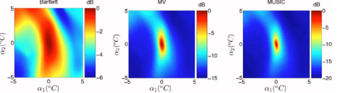
The cost functions were computed as a function of two coefficients ␣1 and ␣2 used to parametrize the temperature profile共see the following details兲 with 关␣1␣2兴T=关00兴Tas true parameter values. Figure1shows the matched-field response of the three BB processors computed for the case assuming coherent spectral components and unknown signal structure. The three plots respectively correspond to implementations of Eqs.共5兲,共6兲, and共10兲, together with Eq.共12兲for estimat-ing the signal matrix. Observestimat-ing Fig. 1, the plot on the left contains a very smooth function as is typical for the Bartlett processor, with a variation between minimum and maximum values of 6 dB. The plot in the middle corresponds to the coherent MV processor, which is clearly superior to the Bar-tlett processor in terms of sidelobe attenuation, with values ranging by about 15 dB. Finally, a plot corresponding to the MUSIC processor was computed. This processor has the best sidelobe attenuation performance of all, with values ranging between −20 and 0 dB. The reader might ask how this was done if this processor approaches⬁ as the parameter vector approaches the true value, under the conditions used for gen-erating the synthetic data. It is possible to portray the MU-SIC processor such that its maximum is 1 by
PMUSIC,1=
␥
␥+ 1
PMUSIC
. 共13兲
It can be seen that PMUSIC,1→1 as PMUSIC→⬁. This modi-fication has two effects:共1兲 The maximum value that can be attained is a known finite value; and 共2兲 implementation al-lows for smoothing the processor. Small values for ␥ will produce a peaky function, while large values for␥will pro-FIG. 1.共Color online兲 The behavior of the broadband processors for the co-herent case assuming an unknown sig-nal matrix.
duce a smooth function. In this study,␥has been always set to 0.01.
Table I summarizes the results obtained in terms of peak-to-surface average ratio for different combinations of coherent/incoherent and known/unknown signal matrix. This measure is the ratio between the surface maximum and its average MF response. It is easy to conclude that there is an increasing discriminating potential when presenting the de-veloped methods in that sequence. The coherent MV proces-sor shows the highest effectiveness in comparison with its incoherent counterpart. For the other two processors coher-ent processing with unknown signal gives similar perfor-mance to incoherent processing with known signal.
B. Error performance
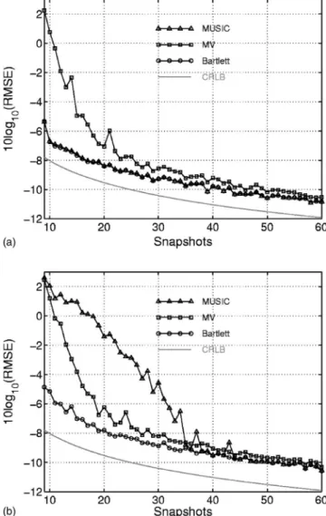
The next issue to be investigated is how the coherent processors perform against the number of signal snapshots N for a given SNR. Here the parameter to be estimated is ␣1, whose true value is 0. Once again the three frequencies/three receivers case is taken with a SNR= 0 dB. Figure 2 shows plots with computations of the RMSE as a function of the number of snapshots N based on 100 estimates of the param-eter. In no case is the Cramer-Rao lower bound attained. Figure2共a兲shows the RMSE with known signal matrix and signal subspace dimension. The MUSIC and Bartlett proces-sors perform similarly for a known signal matrix. The MV processor has poor performance for low number of snapshots and recovers comparatively to the others as the number of snapshots increases. Finally, in the case of unknown signal matrix and signal subspace dimension, Fig.2共b兲shows how the low number of snapshots can impact on the performance of subspace-based methods, in particular, on the separation of the subspaces, in a conjunction with low SNR and low number of snapshots. For the other two processors, working with unknown signal slightly increases the RMSE.
The difficulties seen with the high-resolution methods are related to poor estimates of the eigenvaluesi. The data
model assumes that the eigenvalues associated with the noise subspace are all equal. However, if N is finite, those will be different with probability 1. The MV processor requires in-version of the SDM, whose accuracy depends on the eigen-values’ estimates. Since it weights the eigenvector associated with the smallest eigenvalue most heavily, and this is the least stable vector because it has the least energy and must be orthogonal to all others, a small N is certainly a source of relatively poor performance. Concerning the MUSIC proces-sor, the problem arises when the signal space is to be split into the signal and noise subspaces. This important issue is
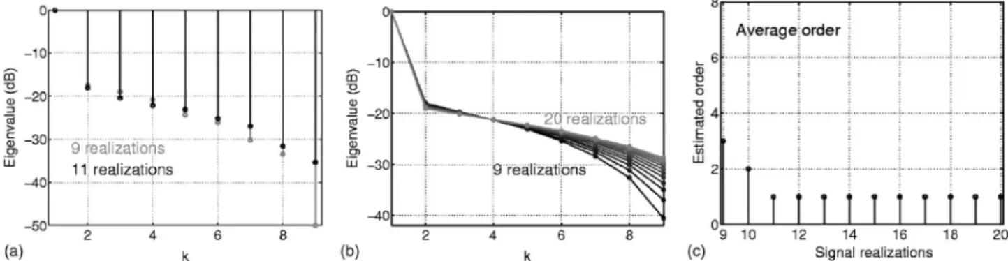
illustrated in Fig.3, which shows in共a兲 the computed eigen-values for two particular cases, one using 9 signal realiza-tions, and the other using 11. The signal subspace dimension is estimated using the MDL criterion.30–32 The former case yields a signal subspace with dimension eight, although a deterministic signal component is used for data generation. Note that the smallest eigenvalue has a very high ratio to its predecessor. The latter case, N = 11, yielded a signal subspace with dimension one—in that case the ratios between contigu-ous higher-order eigenvalues are reduced. Figure3共b兲shows the average eigenspectrum when the number of realizations varies from 9 to 20. For each case 100 realizations of the eigenspectrum were computed and averaged. On average, the eigenspectrum tends to become flattened as N→⬁. Finally, Fig.3共c兲shows the average order estimate obtained using the same data as in Fig. 3共b兲, applying the MDL information criterion. For the minimal number of signal realizations 共9兲 the average order obtained is about 3; for 10 realizations it is about 2; for 11 realizations or more it estimates on average the correct value, which is 1. This exercise illustrates the potential impact of the number of signal realizations on methods relying on the eigendecomposition of the data. TABLE I. Peak-to-surface average ratio obtained for the different
proces-sors. Coherent known signal Coherent unknown ignal Incoherent known signal Incoherent unknown signal Bartlett 2.23 1.86 1.64 1.58 MV 17.9 14.5 6.08 5.41 MUSIC 53.0 41.9 41.9 37.2
FIG. 2. RMSE as a function of the number of snapshots for the three processors and the coherent model Cramer-Rao lower bound under compari-son:共a兲 With known signal matrix and 共b兲 with unknown signal matrix and signal subspace dimension.
C. Global search
In Sec. III A it is shown that all three proposed MF processors significantly differ in their ability of attenuating sidelobes. The next case study is to conclude about the com-parative performance of the processors when the environ-mental estimation problem includes multiple unknown pa-rameters. This problem is usually solved with the aid of a global search method such as a genetic algorithm. The idea is to find out whether high-resolution methods can improve the convergence of meta-heuristic search methods due to their reduced sidelobe structure. Sidelobes competing with the main peak may be seen as false attractors that cause difficul-ties to any meta-heuristic search method in converging to the solution maximizing the cost function.
The data are generated and inverted 50 times using a genetic algorithm. The inversion search space regarded the water column and the seafloor properties, but array tilt was also included. The signal matrix and the signal subspaces dimension were known. The general conditions for synthetic data generation are the same as those used earlier with SNR of 0 dB and 16 snapshots.
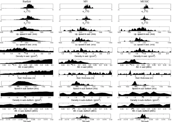
A posteriori distributions can provide insight into the performance of the environmental inversion process. These distributions emphasize the variability of each parameter over the search interval, which is intimately related to the ambiguity pattern of the cost function used and the sensitiv-ity to each parameter. Figure4shows the a posteriori distri-butions obtained for the three methods. To obtain these dis-tributions the individuals of the last generation of all independent populations are merged and histograms are computed from the parameter vectors represented by those individuals.
The idea of showing all these distributions is to obtain a global comparison of the three processors in terms of con-vergence rather than performing a detailed analysis. The MUSIC processor clearly has the narrowest distributions. In fact, that processor contributed to improving the convergence of the genetic algorithm, supporting the belief that a massive sidelobe structure causes difficulties in terms of the popula-tion convergence. The MV processor appears to be more uncertain, which is rather attributed to the problem of invert-ing the SDM with a small N than to the sidelobe structure. Finally, the distributions obtained with the Bartlett processor are significantly more spread out over the search interval
than the others, which is attributed to its massive sidelobe structure causing difficulties for the search algorithm in con-verging to the true solution. From the a posteriori distribu-tions, model estimates based on the distribution peak, called Maximum A Posteriori 共MAP兲 estimates, can be obtained. The MUSIC processor produced more reliable MAP esti-mates, since its parameter distributions are the most com-pact, and all parameters, except sediment upper speed and subbottom density, have a posteriori distributions with a peak close to the true parameter value共indicated by the gray asterisk兲.
IV. ENVIRONMENTAL INVERSION OF EXPERIMENTAL DATA
A. The MREA’03 sea trial
The Maritime Rapid Environmental Assessment 2003 共MREA’03兲 sea trial took place from 26 May to 27 June 2003, in the Ligurian Sea, with target areas North and South of Elba Island. This paper considers only the acoustic experi-ment held on 21 June 200333 whose area of operation was North of the Elba Island as shown in Fig. 5.
1. The deployment geometry
On 21 June, the AOB was deployed on a free drift con-figuration with very favorable weather conditions in an area of mild bottom range-dependency, attaining a variability of 20 m over some acoustic tracks. The experimental setup con-sisted of a towed acoustic source and a free drifting vertical line array with receivers at nominal depths of 15, 60, 75, and 90 m. Figure5共b兲shows the bathymetry in the interior of the white box depicted in the map of Fig.5共a兲together with the source ship navigation and AOB drift estimated from GPS recordings. The acoustic buoy was deployed at 09:01 GMT and recovered at about 15:16 GMT. During this time the buoy drifted about 1.7 km away to the Southeast of the point of deployment, at approximate average displacement of 4.5 m / min共white dashed line兲.
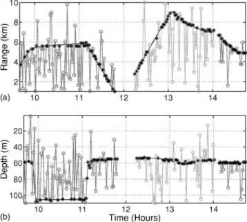
The acoustic source was deployed immediately after the acoustic buoy and towed by the RV Alliance to West where it was stalled between times 09:53 and 11:05 GMT. Then RV Alliance steadily moved to the East and performed the ge-ometry shown in Fig. 5共b兲 共white solid line兲 until source
recovery. Figure 6共a兲 shows the GPS estimated range be-FIG. 3. Eigenspectra for finite number of signal observations:共a兲 Comparison of two eigen-spectra using N=9 共gray兲 and N=11 black; 共b兲 average eigenspectrum for a varying number of signal realizations; and共c兲 average order estimation for a varying number of signal realizations.
tween source and receiver and Fig. 6共b兲 the source depth. The acoustic source was deployed at a variable depth, be-tween 54 and 106 m, depending on ship speed.
2. Acoustic signals
The emitted wave forms consisted of 2-s LFM chirps emitted in two frequency bands. The A1 and A1double chirps are in the band 500– 800 Hz. The signals differ in terms of repetition interval and duty cycle: A1 lasts for 2 s and has a repetition interval of 8 s hence a duty cycle of 25%; A1double lasts for 4 s and has a repetition interval of 10 s hence a duty cycle of 40%. The objective of emitting the A1double wave form was to increase the number of signal realizations in a given observation interval, which may sig-nificantly impact on the performance of some matched-field processors. The A2 chirp is in the band 900– 1200 Hz. Table
IIshows the emission schedule indicating the periods during which each wave form was emitted. The signals were re-ceived at a vertical array containing four hydrophones at nominal depths of 15, 60, 75, and 90 m. Figure7 shows an example of receptions of the A2 chirps at time 11:45 GMT collected at the third receiver. The data are extremely clean without blanks and interruptions, which results from the AOB’s local storage capability. However, it was found that the acoustic data collected by the deepest hydrophone was very noisy most of the time, possibly due to deployment
issues that were not well understood. For this reason it was decided to not consider that hydrophone in the present work. A final remark is that a channel fading effect that signifi-cantly reduces the signal received on the top most hydro-phone was noticed, probably due to the effect of the ther-mocline.
3. Environmental data measurements
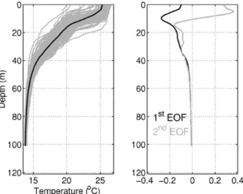
Regarding the inversion of the acoustic data collected on 21 June, 95 conductivity-temperature-depth共CTD兲 measure-ments taken during the days 16, 17, and 19 June taken at the positions marked by the black circles in Fig.5are considered in this study. No CTD measurements were performed during that acoustic experiment since RV Alliance was towing the source. There is a significant difference in scale between the acoustic 共white box兲 and the oceanographic survey, as the latter was set up for different purposes. Those CTD measure-ments are being taken as an attempt to cope with the diffi-culty in sampling the ocean volume, both in time and space, and obtain representative a priori oceanographic data as an input to the acoustic inversion problem. It is of concern to what extent these historical data collected several days be-fore may be representing the oceanography of the target day. Figure 8 shows the measured temperature profiles with two empirical orthogonal functions 共EOF兲 representing more than 80% of the water column variability. The water column FIG. 4. A posteriori probability distributions for each parameter based on the last generation of 50 independent populations. Each column corresponds to processors entering the comparison. The gray asterisks indicate the correct parameter value.
temperature is then modeled as a sum of the mean tempera-ture共thick curve兲 and the two EOFs weighted by associated EOF coefficients␣n. It is useful to measure the coefficients
for the historical data available in order to obtain hints on their range of variation. In the present case␣1 varied in the interval from −15 to 15, and ␣2 varied in the interval from −5 to 5 temperature profiles considered.
4. The environmental model
One of the tasks with the largest impact on the final result is the choice of an adequate environmental model to represent the propagation conditions of the experiment. This choice is generally the result of a compromise between a detailed, accurate, and parameter full model and a light model ensuring a rapid convergence during the processing. The baseline computer model adopted for the MREA’03 was built based on the segmentation of archival bathymetric in-formation along the source-receiver cross sections at differ-ent times. As shown in Fig.5 the bathymetry in the experi-mental area is accurately known. The water depth at the AOB deployment site was approximately 120 m and the maximum depth at the emitting source was 140 m. The base-line geoacoustic properties were drawn from previous studies in that area.10,34 The baseline model consists of an ocean layer overlying a sediment layer and a bottom half space with the bathymetry assumed range dependent, as shown in Fig. 9. The sound-speed profile was calculated using the Mackenzie formula with the mean temperature and mean sa-linity profiles as inputs共see Fig.8兲.
For the purposes of the inversion the forward model was divided into four parameter subsets—water column tempera-ture, sediment, subbottom, and geometric parameters. The temperature in the water column is parametrized by the two EF coefficients as discussed earlier.
B. Results
The following reports on environmental inversions of the experimental acoustic data for water column and seafloor properties using the broadband processors proposed in Sec. II, and the comparison of their estimation performance. FIG. 5.共Color online兲 The Maritime Rapid Environmental Assessment 2003
共MREA’03兲 experimental area: 共a兲 Black circles indicate the sampling grid setup for the CTD measurements used in this study, and the dashed white box limits the area where the acoustic experiment of 21 June took place and 共b兲 GPS estimated source ship navigation 共white solid curve兲 and AOB drift 共white dashed curve兲 during the deployment of 21 June.
FIG. 6. Source range共a兲 and depth 共b兲 measured during the deployment of 21 June. The curves are broken indicating change of the emitted wave form. A1, A2, and A1double denote the wave forms emitted in each interval.
TABLE II. Signal emission schedule on 21 June. The times are in GMT.
Al A2 A1double
Start 09:40 12:14 14:07
End 11:47 14:01 14:44
1. Frequency clustering
The proposed BB matched-field processors are based on the KL⫻KL SDM CYY measuring cross correlations of the
acoustic field across space and frequency. Both the MV and MUSIC processors require CYY to be full-rank, i.e., N艌KL.
If an observation window of 80 s is taken, then the MREA’03 data set provides N = 10 for the A1 and A2 inter-vals, and N = 16 for the A1double interval. Given a number of receivers L = 3 and N = 10, one can choose a number of fre-quencies K = 3 in order to assure that full-rank SDMs are obtained in all emission intervals. In order to use an in-creased number of frequencies while assuring that the SDM is full rank one can use an alternative matched-field proces-sor output given as
PNg共兲 = 1
Ng
兺
n=1 NgP共,n兲. 共14兲
This is an incoherent average over Ng coherent
fre-quency clustersn, where P共,n兲 is a given matched-field
processor. The question is how to choose the frequency
clus-ters. As the idea is to use coherent processors one can carry out an optimization aimed at finding SDMs CYY共n兲 with the
most coherent frequencies. Ideally, one would cluster per-fectly coherent frequencies, which results in a signal sub-space with dimension equal 1. Thus, it appears natural to implement an optimization scheme based on the minimiza-tion of the signal subspace dimension, using an informaminimiza-tion criterion as cost function. Since these criteria are not reliable for N⬇KL it was decided to choose Ng cluster with the
largest1/2—the ratio between the two largest eigenvalues of CYY共n兲 is a simplified measure of the signal’s coherence.
This is a preprocessing step that performs a selection of frequency combinations based on a coherence criterion. In this study a number of clustersNg= 7 will be used, and the
optimization was carried out using a frequency resolution of 4 Hz. In order to assure spectral diversity, frequencies in a cluster are separated by at least 52 Hz.
2. Data processing procedure
Several steps are performed until the inversion is com-plete:
共1兲 Frequency selection based on the 1/2optimization cri-terion.
共2兲 Acoustic field inversion for water column and seafloor properties, and geometric nuisance parameters.
共3兲 Inversion validation by means of source localization with large search bounds using the estimated environ-mental models.
共4兲 Reconstruction of physical parameters of interest using only environmental estimates validated in step共3兲. In step 共2兲 the unknown parameters are divided into water column 共␣1 and␣2 EOF coefficients兲, sediment 共upper and lower compressional speeds, density, attenuation, and thick-ness兲, and subbottom 共compressional speed, density, and at-tenuation兲. Additionally, geometric parameters, array tilt, and receiver depth are included. These parameters are regarded as nuisance parameters, since there is no interest in their estimates once the inversion is finished. The inversion is posed as an optimization problem solved with aid of a ge-netic algorithm共GA兲.35The parameter vector is coded into a 68-bit chain, which results in a search space size approxi-mately equal to 2.95⫻1020. The GA settings are summarized in TableIII. Since there is a new time bin every 80 s only a single population is used for each inversion, which is suffi-cient to achieve the main objective of comparing the pro-posed MF processors’ inversion performance.
FIG. 8. CTD-based data used for temperature estimation taken during 16, 17, and 19 June Temperature profiles with mean profile in solid black共left兲 and representative empirical orthogonal functions共EOF兲 computed from the temperature profiles共right兲.
FIG. 9. Baseline model for the MREA’03 sea trial. All parameters except water depth are range independent.
TABLE III. GA settings for environmental inversion.
Parameter Setting Generations 30 Population size 200 Independent populations 1 Mutation probability 0.004 Crossover probability 0.9
Step 共3兲 is to validate the model estimates obtained in step 共2兲 by means of range-depth source localization. This step is based on the accurate knowledge on source range and depth available and on the fact that source position is on top of the parameter hierarchy. It is assumed that if the environ-mental estimates are not accurate then the source cannot be properly located. Performing source localization with large search bounds should give an indication on the quality of a given environmental estimate.
Finally, step 共4兲 is to produce the final environmental estimates using only those estimates validated in step共3兲.
3. Environmental inversion: Comparison of three MF processors
Here, the three BB processors will be applied to experi-mental field data. The whole data set collected on 2l June will be inverted with each processor. In Sec. III C, inversions on synthetic data with a GA indicated that high-resolution processors may contribute to improve the convergence to the true solution. The comparison performed here may also serve the purpose of understanding how these processors behave in a real situation with the inherent model mismatch. The maxi-mum source-receiver range is 9 km, which is more than 70 water depths, possibly giving rise to environmental mis-match.
The inversion is carried out assuming an unknown sig-nal matrix CSS. Since the frequencies are optimized in the
sense of clustering those with highest coherence, it is as-sumed that the signal subspace dimension is always one, although source and receiver are moving most of the time. The processing is, therefore, considered broadband coherent with unknown wave form.
No ground truth measurements are available for evalu-ating the inversion performance achieved. Thus, one can re-fer directly to step共3兲, the validation step, and analyze those results. Source localization along time was performed within search bounds from 1 to 10 km in range, and from 1 to 110 m in depth. The source is admitted as correctly localized if the error both in range and depth is simultaneously less than 5% of the search interval amplitude. In other words the maximum must fall in a 0.9-km-long and 11-m-wide rect-angle centered on the true location. TableIVshows the rate of successful localization achieved with each processor. The localization rate was computed for each emission interval due to the different signal characteristics, and then summa-rized on the rightmost column as an overall result. Consid-ering the overall results, the MUSIC processor clearly out-performs the other two processors, as the localization rate increases with the processors’ resolution. A more detailed analysis of the result allows for making the following
re-marks: 共i兲 The A1 interval was the most difficult. Close in-spection shows that the localization rate is clearly lower with the source stalled at 105 m 共during time 10:00 to 11:00兲 in the three cases.共ii兲 The MV processor performed remarkably well during the A1double interval. It appears that this pro-cessor performed particularly well with the number of signal realizations N = 16 provided by that data portion, while show-ing difficulties in the other data portions providshow-ing N = 10 共which is consistent with the synthetic study兲. 共iii兲 The source was located both in range and depth at ranges up to 9 km, as indicated by the black asterisks in Fig.10.
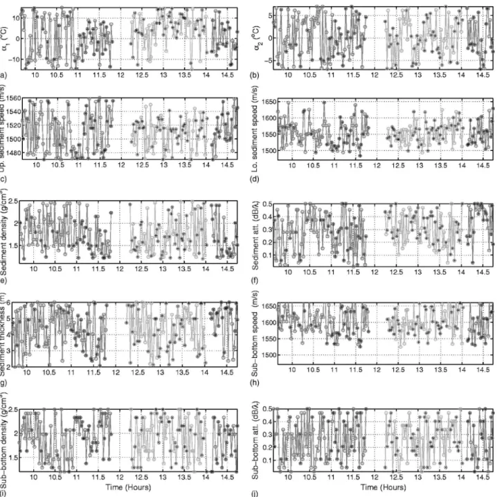
Figure11shows the environmental inversion results ob-tained with the MUSIC processor. The reason for showing the run performed with the MUSIC processor was its overall superiority in terms of source localization, and the belief that this means that the environmental estimations are also of superior quality in comparison with those obtained with the other processors. The circles filled with an asterisk corre-spond to inversions with successful localization.
It can be seen in plot 共a兲 that from time 10:00 to time 11:00 the estimate of the ␣1 EOF coefficient, a leading pa-rameter, varies over the entire search interval. When the source moves and goes up to approximately midwater col-umn, the variability substantially reduces, with the estimates becoming confined in the interval −10 to 10. During A2 the estimates continue in the interval −10 to 10 at the beginning but then during the remaining part the estimates are in the upper half of the search interval between 0 and 15. Finally, the ␣1 estimates in the A1double period are clearly in the interval −10 to 10. The second EOF coefficient was searched in an interval with amplitude less than half of that for the first one. The EOFs used to model the water column differ significantly only in the first third of the water column, while they coincide for the remaining depth. On the other hand only one receiver is in place in the first third of the water TABLE IV. Rates of successful localization共%兲 for the different processors
and different wave forms.
Processor A1 A2 A1double Overall Bartlett 22.7 38.3 51.9 32.7
MV 22.7 29.6 85.2 35.1
MUSIC 39.0 53.1 70.4 48.3
FIG. 10. Source localization obtained with the MUSIC processor. Source range共a兲 and source depth 共b兲. True location is given by the black curve in the background. The gray curves with circles are the source localization results. The black asterisks indicate the successful localizations.
column. In Ref.36it is shown that these circumstances lead to an ambiguous cost function regarding the ␣i coefficients,
resulting in a poor solution uniqueness.
Concerning the seafloor parameter estimates, most of them appear to be unstable, making it nearly impossible to draw some value from the plots of Fig.11. Nevertheless, the compressional speeds in sediment and subbottom appear to be fairly restricted to subintervals in the search interval with aid of the source localization step. In order to obtain a single estimate for each of the seafloor parameters, a posteriori distributions based on the individuals of the last generation of each inversion allowing for correct source localization共43 out of 81 inversions兲 were computed considering only the A2 emission period共see Fig.12兲. Sediment and subbottom
com-pressional speeds, and sediment attenuation are relatively
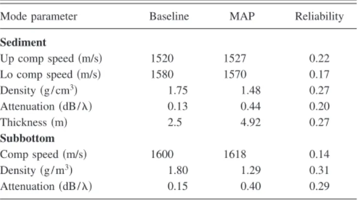
compact, each with a peak close to the baseline value. Also, sediment density and thickness show an outstanding distri-bution peak. The sediment attenuation distridistri-bution, although compact, is concentrated at the upper search bound far from the baseline value. Table Vcontains the MAP estimates for the seafloor parameters, together with the baseline values and a measure of the estimation reliability, which is the standard deviation of the a posteriori distribution divided by the search interval length. The MAP estimates of the compres-sional speeds are in fair agreement with the baseline values. Sediment density and thickness are also credible.
Finally, it can be remarked that during the A2 emission period, the MUSIC processor produced the most reliable en-vironmental estimates. During the A1double emission period the most reliable environmental estimates were produced by FIG. 11. Model parameter estimates obtained via acoustic data inversion using the BB MUSIC processor. Water column关共a兲 and 共b兲兴; sediment 关共c兲–共g兲兴; and subbottom关共h兲–共j兲兴. The black asterisks indicate model estimates allowing for successful source localization in the validation step.
the MV processor. This supports the close relation between the rate of source localization and the quality of the environ-mental estimation, and the choice of source localization as a validation tool.
V. CONCLUSIONS
Acoustic data were collected using a prototype of a light acoustic receiving system, an AOB, developed to meet op-erational requirements such that it consisted of a vertical line array with only three operating receivers. One of the objec-tives of these acoustic data was to evaluate the performance of newly adapted field inversion methods for the estimation of water column and geoacoustic properties using such a light acoustic receiving system.
The application of genetic algorithms for the estimation of model parameters has been shown to be very effective on several occasions. However, when a sparse receiving array is used the inversion problem becomes heavily ill-conditioned. Traditionally, the difficulty of solving an ill-conditioned problem has been associated with model mismatch and noise, which may lead to the situation where the optimum is not in coincidence with 共or even close to兲 the true model parameters.
This paper associates this difficulty with the application of a genetic algorithm to carry out the optimization, specifi-cally due to the existence of many local extrema in concur-rence with the main peak, together with the typically large search space of a multiple environmental estimation prob-lem. In order to cope with this difficulty broadband matched-field processors, specifically, high-resolution processors, are proposed for their increased ability in attenuating sidelobes. A Bartlett, a minimum-variance, and MUSIC processor, all truly broadband rather than a superposition of multiple frequencies since they are based on a broadband data model, were first compared in terms of estimation performance with synthetic data. It was concluded that in the case of an ex-haustive search of the unknown parameter, the high-resolution processors were unable to outperform the Bartlett processor. The main difficulty of the application of the high-resolution processors is related to a reduced number of signal realizations to compute the sample spectral density matrix 共SDM兲. In the case of a multiparameter inversion problem the comparison shows that the high-resolution methods
clearly contribute to improve the convergence of the genetic algorithm to the true model parameters, therefore reducing the inherent uncertainty.
The inversion results with the experimental data are con-sistent with those obtained with the synthetic data in terms of processor performance comparison. The inversion algorithm included a source localization step with large search bounds aimed at discarding model estimates upon wrong localization result. As no concurrent environmental ground truth data were available the processor performance was evaluated by means of the rate of correct source localization. Based on that criteria, the MUSIC processor achieved the best overall performance. Note that this processor was applied assuming that the dimension of the signal subspace was one, since a coherence optimization step was performed before. This con-tributed to avoiding a major difficulty with this processor— the estimation of the signal subspace dimension. The minimum-variance processor achieved an exceptional perfor-mance in an emission interval where a larger number of sig-nal realizations were available. With this data set successful source localization results were obtained for ranges up to 9 km.
FIG. 12. A posteriori probability distributions for the seafloor parameters based on the last generation of the GA. Only inversions validated by means of source localization during the A2 period are considered. The gray asterisk indicates the baseline value of the parameter.
TABLE V. Baseline seafloor parameters, parameter MAP estimates on 43 GA populations, and a reliability measure.
Mode parameter Baseline MAP Reliability
Sediment Up comp speed共m/s兲 1520 1527 0.22 Lo comp speed共m/s兲 1580 1570 0.17 Density共g/cm3兲 1.75 1.48 0.27 Attenuation共dB/兲 0.13 0.44 0.20 Thickness共m兲 2.5 4.92 0.27 Subbottom Comp speed共m/s兲 1600 1618 0.14 Density共g/m3兲 1.80 1.29 0.31 Attenuation共dB/兲 0.15 0.40 0.29
The EOF coefficients, used to parametrize the water col-umn, were estimated with some uncertainty, although well restricted to subintervals over some periods. A single esti-mate of the seafloor properties was obtained by means of the maximization of the a posteriori distributions based on the last populations of the genetic algorithm. This result is es-sentially in line with the baseline model values for compres-sional speeds in the sediment and subbottom, and density in the sediment. The estimate of the sediment thickness is also well determined. Finally, a strong relation between uncer-tainty and source localization rate was observed共Fig.12兲.
The dimension of the search space appears to be a major impairment for consistently obtaining valid model estimates 共by means of correct source localization兲 over time since, in principle, this cannot be attributed to model mismatch or additive noise.
ACKNOWLEDGMENTS
The authors would like to thank the NATO Undersea Research Centre for the organization of the MREA’03 sea trial. This work was financed by FCT, Portugal, under fel-lowship SFRH/BD/12656/2003 and NUACE project, Con-tract No. POSI/CPS/47824/2002, and the development of the AOB prototype was funded by the Portuguese Ministery of Defense under the LOCAPASS project.
1A. Tolstoy, Matched Field Processing for Underwater Acoustics共World
Scientific, Singapore, 1993兲.
2A. B. Baggeroer, W. A. Kuperman, and P. N. Mikhalevsky, “An overview
of matched field methods in ocean acoustics,” IEEE J. Ocean. Eng. 18, 401–424共1993兲.
3H. P. Bucker, “Use of calculated sound fields and matched-detection to
locate sound source in shallow water,” J. Acoust. Soc. Am. 59, 368–373 共1976兲.
4A. Tolstoy, O. Diachok, and N. L. Frazer, “Acoustic tomography via
matched field processing,” J. Acoust. Soc. Am. 89, 1119–1127共1991兲.
5M. D. Collins, W. A. Kuperman, and H. Schmidt, “Nonliear inversion for
ocean-bottom properties,” J. Acoust. Soc. Am. 92, 2770–2783共1992兲.
6P. Gerstoft, “Inversion of acoustic data using a combination of genetic
algorithms and the Gauss-Newton approach,” J. Acoust. Soc. Am. 97, 2181–2190共1995兲.
7S. E. Dosso, M. L. Yeremy, J. M. Ozard, and N. R. Chapman, “Estimation
of ocean-bottom properties by matched-field inversion of acoustic field data,” IEEE J. Ocean. Eng. OE-18, 232–239共1993兲.
8C. E. Lindsay and N. R. Chapman, “Estimation of ocean-bottom
proper-ties by matched-field inversion of acoustic field data,” IEEE J. Ocean. Eng. OE-18, 224–231共1993兲.
9M. D. Collins and W. A. Kuperman, “Focalization: Environmental
focus-ing and source localization,” J. Acoust. Soc. Am. 90, 1410–1422共1991兲.
10D. F. Gingras and P. Gerstoft, “Inversion for geometric parameters in
shallow water: Experimental results,” J. Acoust. Soc. Am. 97, 3589–3598 共1995兲.
11P. Gerstoft and D. Gingras, “Parameter estimation using multi-frequency
range dependent acoustic data in shallow water,” J. Acoust. Soc. Am. 99, 2839–2850共1996兲.
12C. Soares, M. Siderius, and S. M. Jesus, “Source localization in a
time-varying ocean waveguide,” J. Acoust. Soc. Am. 112, 1879–1889共2002兲.
13M. Snellen, D. G. Simons, M. Siderius, J. Sellschopp, and P. L. Nielsen,
“An evaluation of the accuracy of shallow water matched field inversion results,” J. Acoust. Soc. Am. 109, 514–527共2001兲.
14R. M. Hamson and R. M. Heitmeyer, “An analytical study of the effects of
environmental and system parameters on source localization in shallow
water by matched-field processing of a vertical array,” J. Acoust. Soc. Am.
86, 1950–1959共1989兲.
15A. B. Baggeroer, W. A. Kuperman, and H. Schmidt, “Matched field
pro-cessing: Source localization in correlated noise as an optimum parameter estimation problem,” J. Acoust. Soc. Am. 80, 571–587共1998兲.
16A. Tolstoy, “Computational aspects of matched field processing in
under-water acoustics,” in Computational Acoustics, edited by D. Lee, A. Cak-mak, and R. Vichnevetsky共North-Holland, Amsterdam, 1990兲, Vol. 3, pp. 303–310.
17Z.-H. Michalopoulou, “Matched-field processing for broad-band source
localization,” IEEE J. Ocean. Eng. 21, 384–392共1996兲.
18Z.-H. Michalopoulou, “Source tracking in the Hudson Canyon
experi-ment,” J. Comput. Acoust. 4, 371–383共1996兲.
19G. J. Orris, M. Nicholas, and J. S. Perkins, “The matched-phase coherent
multi-frequency matched field processor,” J. Acoust. Soc. Am. 107, 2563– 2575共2000兲.
20C. Soares and S. M. Jesus, “Broadband matched field processing:
Coher-ent and incoherCoher-ent approaches,” J. Acoust. Soc. Am. 113, 2587–2598 共2003兲.
21A. Silva, F. Zabel, and C. Martins, “Acoustic oceanographic buoy: A
telemetry system that meets rapid environmental assessment require-ments,” Sea Technol. 47, 15–20共2006兲.
22S. M. Jessus, C. Soares, E. Coelho, and P. Picco, “An experimental
dem-onstration of blind ocean acoustic tomography,” J. Acoust. Soc. Am. 3, 1420–1431共2006兲.
23J. Capon, “High-resolution frequency-wavenumber spectrum analysis,”
Proc. IEEE 57, 1408–1418共1969兲.
24R. O. Schmidt, “A signal subspace approach to multiple emitter location
and spectral estimation,” Ph.D. dissertation, Stanford University, Stanford, CA, 1982.
25K. Hsu and A. B. Baggeroer, “Application of the maximum-likelihood
method 共mlm兲 for sonic velocity logging,” Geophysics 51, 780–787 共1986兲.
26P. C. Mignerey and S. Finette, “Multichannel deconvolution of an acoustic
transient in an oceanic waveguide,” J. Acoust. Soc. Am. 92, 351–364 共1992兲.
27S. Finette, P. C. Mignerey, J. F. Smith, and C. D. Richmond, “Broadband
source signature extraction using a vertical array,” J. Acoust. Soc. Am. 94, 309–318共1993兲.
28J. F. Boehme, Advances in Spectrum Analysis and Array Processing,
共Prentice Hall, Englewood Cliffs, NJ, 1991兲, Vol. 2, Chap. 1, pp. 1–63.
29C. M. Ferla, M. B. Porter, and F. B. Jensen, “C-SNAP: Coupled
SACLANTCEN normal mode propagation loss model,” Memorandum SM-274, SACLANTCEN Undersea Research Center, La Spezia, Italy, 1993.
30G. Schwartz, “Estimating the dimension of a model,” Ann. Stat. 6, 461–
464共1978兲.
31J. Rissanen, “Modeling by shortest data description,” Automatica 14, 465–
471共1978兲.
32M. Wax and T. Kailath, “Detection of signals by information theoretic
criteria,” IEEE Trans. Acoust., Speech, Signal Process. ASSP-33, 387–392 共1985兲.
33S. Jesus, A. Silva, and C. Soares, “Acoustic Oceanographic Buoy test
during the MREA’03 sea trial,” Internal Rep. 04/03, SiPLAB/CINTAL, Universidade do Algarve, Faro, Portugal, November 2003.
34F. B. Jensen, “Comparison of transmission loss data for different
shallow-water areas with theoretical results provided by a three-fluid normal-mode propagation mode,” in Sound Propagation in Shallow Water, edited by O. F. Hastrup and O. V. Oleson共SACLANT Undersea Research Centre, La Spezia, Italy, 1974兲, Vol. II, pp. 79–92, SACLANTCEN document CP-14.
35T. Fassbender, “Erweiterte genetische algorithmen zur globalen
optim-ierung multi-modaler funktionen共Extended genetic algorithms for global optimization of multi-modal functions兲.” Diplomarbeit, Ruhr-Universität, Bochum, 1995.
36C. Soares, S. M. Jesus, and E. Coelho, “Acoustic oceanographic buoy
testing during the maritime rapid environmental assessment 2003 sea trial,” in Proceedings of the European Conference on Underwater