Maximum Level and Time to Peak of Dam-Break Waves on
Mobile Horizontal Bed
João G. A. B. Leal
1; Rui M. L. Ferreira
2; and António H. Cardoso
3Abstract:This experimental study focuses the influence of bed material mobility and initial downstream water level on maximum water level and time to peak of dam-break waves. It covers horizontal bed conditions on fixed bed, sand bed, and pumice bed. Results include water surface level time evolution, maxima wave levels and time to peak. The influence of bed material mobility and downstream water level was identified and characterized, stressing the importance of using mathematical models with appropriate sediment transport formulations instead of purely hydrodynamic models to simulate dam-break waves on mobile bed channels.
DOI:10.1061/共ASCE兲HY.1943-7900.0000099
CE Database subject headings:Dams; Water waves; Bed materials; Sediment transport.
Introduction
The most important features of dam-break flows 共DBF兲 are the maximum wave level and time to peak. Lauber and Hager共1998兲
have characterized experimentally these variables for fixed, hori-zontal, initially dry bed downstream the dam, taking into consid-eration the influence of the upstream reservoir length.
Recent events and observations point out that DBF can interact strongly with the mobile bed, causing major impacts in its mor-phology. This was the case, for instance, downstream of Lake Ha! Ha! due to the rupture of a dyke 共Lapointe et al. 1998兲. The occurrence of intense sediment transport in DBF as well as the interaction between the flow and the bed can significantly affect the flow dynamics, usually contributing to increase the water sur-face levels and to decrease the wave-front celerity as compared with purely hydrodynamic solutions共cf. Leal et al. 2006兲. Never-theless, such solutions are frequently used due to difficulties in the implementation and exploitation of models accounting for the bed mobility.
The role of bed mobility in DBF was scarcely studied in the past. For lightweight granular bed material, Capart and Young
共1998兲observed the excavation of a scour hole near the dam cross section, leading to the onset of an hydraulic jump. Spinewine and Zech共2007兲concluded that the scour hole and the hydraulic jump were significantly attenuated for heavier, less mobile bed. The effect of the water level downstream the dam was rarely studied
too. Stansby et al. 共1998兲and Leal et al.共2002兲verified that the water surface level behind the wave-front raises as compared with the pure hydrodynamic solution, creating a jump whose height increases with the initial downstream water level. The present experimental study intends to contribute to further characterize the influence of bed mobility and initial water level downstream the dam on maximum wave level and time to peak in horizontal, mobile bed channels.
Experiments
The data used in this study were collected by Leal共2005兲. Tests were carried out in a 19.2-m long, 0.5-m wide, and 0.7-m high rectangular flume with horizontal bed. For simulating dam-break events, a vertical lift-gate, installed in the middle cross section of the flume, was opened instantaneously. Three types of bed were adopted: fixed bed, sand bed, and pumice bed. The sand diameter wasds= 0.8 mm; sand specific gravity wass= 2.65. For pumice,
these variables were 1.2 mm and 1.40, respectively. The initial water depth upstream the gate was the same in all tests 共hu
= 0.40 m兲; for mobile bed tests, the initial bed elevation was al-ways kept equal to 0.07 m, both up and downstream the gate; the initial water depth downstream,hd, ranged from 0.000–0.210 m. The main features of the initial conditions are summarized in Table 1, where ␣=hd/huis the dimensionless initial downstream
water depth. Assuming hydrostatic pressure distribution, the time evolution of water surface levels was measured with seven pres-sure transducers installed downstream the gate, atX= 0.5, 2.5, 5.0, 7.5, 12.5, 17.5, and 22.5, whereX=x/huandx= longitudinal co-ordinate measured from dam cross section.
Time Evolution of Water Surface Level
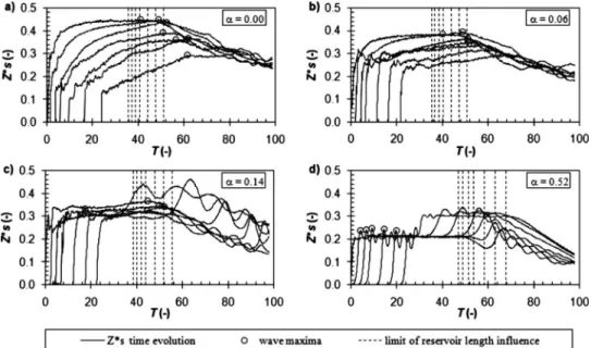
Fig. 1 presents the time evolution of dimensionless water surface levels,Zsⴱ, of fixed bed tests,␣= 0.00, 0.06, 0.14, and 0.52. In Fig.
1,Zsⴱ=z s ⴱ/hu;z
s
ⴱ= measured water surface elevation above the
ini-tial water level downstream the gate; T=t/共hu/g兲0.5 = dimensionless time; t= time; g= gravitational acceleration. The maxima wave levels are marked with circles; the instants of 1
Assistant Professor, Dept. of Civil Engineering, Faculty of Sciences and Technology, Universidade Nova de Lisboa, Quinta da Torre, Caparica 2829-516, Portugal共corresponding author兲. E-mail: [email protected]
2
Assistant Professor, Dept. of Civil Engineering and Architecture, Instituto Superior Técnico, UTL, Av. Rovisco Pais, Lisbon 1049-001, Portugal. E-mail: [email protected]
3
Full Professor, Dept. of Civil Engineering and Architecture, Instituto Superior Técnico, UTL, Av. Rovisco Pais, Lisbon 1049-001, Portugal. E-mail: [email protected]
time—time limits—above which the limited upstream reservoir length starts to influence the wave levels at the measuring cross sections are also identified with vertical dashed lines. Time limits were calculated by assuming that the negative wave-front celeri-ties measured by Leal et al.共2002兲also apply downstream. For a given location, X, the time limit is therefore computed as 共2r
+X兲/C
NF, where r=Lr/hu= dimensionless reservoir length; Lr
= length of the upstream reservoir;CNF= dimensionless negative wave-front celerity.
For the lower values of␣关␣= 0.00, Fig. 1共a兲, and␣= 0.06, Fig. 1共b兲兴, the water surface level rises abruptly, in each section, im-mediately after the arrival of the wave-front; afterwards, it in-creases slowly until reaching the maximum; afterwards, the water level decreases slowly as the upstream reservoir empties. This behavior was also observed by Lauber and Hager共1998兲for fixed horizontal bed. For higher values of ␣ 关␣= 0.14, Fig. 1共c兲, and
␣= 0.52, Fig. 1共d兲兴, water levels are influenced, after some time, by reflection waves induced by the downstream weir used to guar-antee the water level downstream the gate. Whenever this oc-curred the “corrupted” parts of the records were ignored in the analysis. As ␣ increases, the maxima wave levels are attained
sooner and tend to become independent of the reservoir length, i.e., they occur before the calculated time limit. For the highest value of ␣ 关␣= 0.52, Fig. 1共d兲兴 the maxima wave levels are at-tained just after the arrival of the wave-front due to the fact that the wave propagates downstream as a solitary wave or as a group of waves共cf. Leal 2005兲.
For sand bed, the time evolution of the water surface elevation is practically as described above. Still, the maxima wave levels at X= 0.5 are attained slightly sooner共cf. Leal 2005兲.
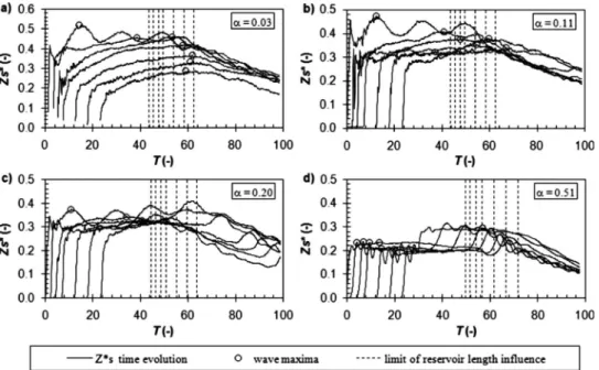
Fig. 2 presents the time evolution of the dimensionless water surface levels of pumice bed tests,␣= 0.03, 0.11, 0.20 and 0.51. Again, the water surface behavior presents qualitative similarities with the one described for fixed bed. Important discrepancies are observed, however, at the cross section the nearest to the gate for the lower ␣ values 关Figs. 2共a and b兲兴, where the water surface level does not rise slowly until reaching its maximum. Instead, it exhibits an oscillatory behavior; the maximum level is attained much sooner than for the other sections and is independent of the reservoir length. It can be concluded that, for locations near the gate, the increase of bed mobility induces the increase of the water surface levels. Although this can be attributed to the added Table 1.Tests Main Features
Test Type of bed
hd 共m兲
␣
共⫺兲 Test Type of bed
hd 共m兲
␣ 共⫺兲
Ts.1 Sandds= 0.8 mms= 2.65 0.003 0.01
T.1 fixed bed 0.000 0.00 Ts.2 0.012 0.03
T.2 0.023 0.06 Ts.3 0.042 0.10
T.3 0.049 0.12 Ts.4 0.073 0.18
T.4 0.056 0.14 Ts.5 0.106 0.26
T.5 0.071 0.18 Ts.6 0.204 0.51
T.6 0.082 0.20 Tp.1 Pumiceds= 1.2 mms= 1.40 0.013 0.03
T.7 0.094 0.23 Tp.2 0.014 0.04
T.8 0.114 0.28 Tp.3 0.044 0.11
T.9 0.142 0.35 Tp.4 0.078 0.20
T.10 0.212 0.52 Tp.5 0.107 0.27
Tp.6 0.207 0.51
Fig. 1. Time evolution of dimensionless water level,Zsⴱ, at X= 0.5, 2.5, 5.0, 7.5, 12.5, 17.5 and 22.5共right to left兲for fixed bed tests: 共a兲 ␣
sediment inertia and to the increase of flow resistance, it should be mostly dictated by morphological changes—scour hole— observed in the bed profile共cf. Leal 2005兲.
Maxima Wave Levels
It was found that maxima wave levels, 共Zsⴱ兲max, can be fitted by
the following relation
1/共Z
s ⴱ兲max=共a
1␣+a3兲X+共a2␣+a4兲 共1兲
wherea1,a2,a3anda4= regressions coefficients which depend on
the bed type, according to Table 2. Fig. 3 plots Eq.共1兲against the experimental data. The equation proposed by Lauber and Hager
共1998兲for fixed, horizontal dry bed
共Zsⴱ兲max=4
9
冉
1 + 1Xⴱ
冊
−5/4共2兲
where Xⴱ=rX−2/3, is also included in Fig. 3共a兲. For fixed and
sand bed tests, ␣ ⬍⬇0.2, as well as for pumice bed tests, ␣ ⬍
⬇0.3, 1/共Z
s
ⴱ兲max increases linearly with X, i.e., the maximum
water surface elevation decreases withX. This can be attributed to the finite length of the reservoir and is in accordance with re-ported real cases. However, for higher values of␣, waves behave as solitary waves or groups of waves, the kinetic energy converts into potential energy through the increase of the water surface elevation and the influence of the upstream reservoir length ulti-mately ceases. The influence of the initial downstream water level
共i.e.,␣兲decays with X, since, for high Xvalues, maxima water
Fig. 2.Time evolution of dimensionless water level,Zsⴱ, atX= 0.5, 2.5, 5.0, 7.5, 12.5, 17.5 and 22.5共right to left兲for pumice bed tests:共a兲␣
= 0.03;共b兲␣= 0.11;共c兲␣= 0.20; and共d兲␣= 0.51
Table 2.Regression Coefficients of Eq.共1兲
Type of bed
a1 共⫺兲
a2 共⫺兲
a3 共⫺兲
a4 共⫺兲
Fixed ⫺0.2233 4.3681 0.0431 2.2354
Sand ⫺0.2598 4.4543 0.0630 2.0880
Pumice ⫺0.1894 5.1618 0.0744 1.7340
Fig. 3.Variation of dimensionless maximum wave level, 1/共Z s ⴱ兲
surface levels tend to a constant value irrespective of␣. Although the described behavior applies to the three bed types, pumice bed results are somewhat different from fixed bed and sand bed. For small values of␣, the water surface level is slightly
higher, which is in accordance to what was mentioned before, i.e., the bed morphological changes and the flow-bed interaction in-crease the maxima wave levels, especially near the gate cross section.
Time to Peak
Fig. 4 presents the variation of the dimensionless time to peak, Tⴱ=T
maxX−2
/3
, withX.Tmax=tmax共g/hu兲1
/2
;tmax= time to peak,
as-sociated to the maximum water level. The equation proposed by Lauber and Hager 共1998兲 for fixed, horizontal dry bed is also plotted
Tⴱ= 1.7共1 +Xⴱ兲 共3兲
From Fig. 4, it can be concluded that the equation of Lauber and Hager共1998兲is a rather good predictor as soon as␣ ⬍⬇0.14 and
Xⴱ⬍15. Since higher values ofXⴱ correspond to cross sections
located near the gate, it can also be concluded that the morpho-logical changes occurring in the mobile bed influence mostly the time to peak at those sections. For high ␣ values, the wave maxima levels are attained shortly after the wave-front arrival. Nevertheless, the influence of the water depth downstream 共i.e.,
␣兲on time to peak is smaller asXⴱdecreases.
Conclusions
From the previous sections and within the range of covered ex-perimental conditions, the following conclusions can be drawn:
共1兲 maxima wave levels near the gate are higher and attained sooner for highly movable bed material 共pumice兲 as compared with fixed bed, and become independent of the upstream reservoir length;共2兲for small initial water depth downstream the gate, the maxima wave levels decrease in the downstream direction, while the opposite trend is observed for high initial water depth;共3兲the influence of the water depth downstream—expressed by ␣—on
the amplitude of water level variations and on time to peak is attenuated in the downstream direction.
These results stress the importance of using mathematical models incorporating appropriate sediment transport formulations instead of purely hydrodynamic models to propagate dam-break waves on mobile bed channels.
Acknowledgments
The writers wish to acknowledge the financial support of the Por-tuguese Foundation for Science and Technology through the Grant Nos. POCTI/36069/ECM/99 and PTDC/ECM/70652/2006.
Notation
The following symbols are used in this technical note: a1,a2,a3,a4 ⫽ regressions coefficients of Eq.共1兲;
CNF ⫽ dimensionless celerity of the negative
wave-front;
ds ⫽ sediment mean diameter; g ⫽ gravitational acceleration; h ⫽ flow depth;
hd ⫽ initial water depth downstream; hu ⫽ initial water depth upstream; Lr ⫽ upstream reservoir length;
s ⫽ sediment specific gravity;
T ⫽ dimensionless time after the dam-break;
Tⴱ ⫽ dimensionless time to peak defined as TmaxX−2
/3;
Tmax ⫽ dimensionless time to peak; t ⫽ time after the dam-break;
tmax ⫽ time to peak;
X ⫽ dimensionless location from the dam; Xⴱ ⫽ dimensionless length parameter defined as
rX−2/3
;
x ⫽ location from the dam section; Zsⴱ ⫽ dimensionless water surface elevation
measured from the initial water level downstream of the dam;
zsⴱ ⫽ water surface elevation measured from the
initial water level downstream of the dam;
Fig. 4.Variation of dimensionless time to peak,Tⴱ, withXⴱ:共a兲fixed
␣ ⫽ dimensionless initial downstream water depth; and
r ⫽ dimensionless upstream reservoir length.
References
Capart, H., and Young, D. L.共1998兲. “Formation of a jump by the dam-break wave over a granular bed.”J. Fluid Mech., 372, 165–187. Lapointe, M. F., Secretan, Y., Driscoll, S., Bergeron, N., and Leclerc, M.
共1998兲. “Response of the Ha! Ha! River to the flood of July 1996 in the Saguenay Region of Quebec: Large-scale avulsion in a glaciated valley.”Water Resour. Res., 34, 2383–2392.
Lauber, G., and Hager, W. H.共1998兲. “Experiments to dambreak wave: Horizontal channel.”J. Hydraul. Res., 36共3兲, 291–307.
Leal, J. G. A. B.共2005兲. “Experimental and mathematical modeling of dam-break waves over mobile bed open channels.” Ph.D. thesis, Uni-versidade da Beira Interior, Covilhã, Portugal共in Portuguese兲. Leal, J. G. A. B., Ferreira, R. M. L., and Cardoso, A. H.共2002兲.
“Dam-break waves on movable bed.” Proc., of the Int. Conf. on Fluvial Hydraulics, Balkema, Rotterdam, The Netherlands, 981–990. Leal, J. G. A. B., Ferreira, R. M. L., and Cardoso, A. H.共2006兲.
“Dam-break wave-front celerity.”J. Hydraul. Eng., 132共1兲, 69–76. Spinewine, B., and Zech, Y.共2007兲. “Small-scale laboratory dam-break
waves on movable beds.”J. Hydraul. Res., 45共Extra Issue兲, 73–86. Stansby, P. K., Chegini, A., and Barnes, T. C. D. 共1998兲. “The initial