Dissertation
Master in Medical Information Systems Management
Exporting data from an openEHR repository
to standard formats
Jorge Daniel Borges Brilhante Almeida
Dissertation
Master in Medical Information Systems Management
Exporting data from an openEHR repository to
standard formats
Jorge Daniel Borges Brilhante Almeida
Masters dissertation performed under supervision of Doutor Ricardo João Cruz-Correia, Professor of School of Management and Technology from Leiria Polytechnic Institute and
the Faculty of Medicine of the Oporto University
ii
iii
“Declare the past, diagnose the present, foretell the future.”
Hippocrates
“Arguably the greatest technological triumph of the century has been the public-health system, which is sophisticated preventive and investigative medicine organized around mostly low- and medium-tech equipment; ... fully half of us are alive today because of the improvements.”
iv
v
Acknowledgements
To my son, who gave me the strength to endure during the long and lonely nights of writing. To my friends and family for their patience and support.
To Professor Ricardo Correia and Samuel Frade for their guidance, dedication, collaboration and availability throughout this stage.
And finally, to everyone who have in some way contributed so that this thesis could be concluded.
vi
vii
Abstract
With the healthcare sector computerization, a large amount of data is produced from medical encounters, therapeutic outcomes and other aspects of healthcare provider’s organizations current activity. Decision support systems cover several methodologies and approaches that may be applied to the healthcare sector and, since that they store and analyze data in a tabular format, it becomes necessary to assure that data sources with different data representations can be used to feed these systems.
The present work focuses on the development of a methodology to export data from an openEHR repository to standard formats through a software tool which adapts itself to different data sources for later exploration in statistical and decision support systems. From use case and requirements analysis to the efective development of the tool, several steps were performed to document progress and to ground conclusions regarding operational test data.
Obtained results indicate that this data export is feasible, but also highlight the need to define parameters so that the tool may function.
viii
ix
Resumo
Com a informatização do sector da saúde, uma grande quantidade de dados é produzida a partir de encontros médicos, resultados terapêuticos e outros aspectos da actividade corrente dos prestadores de cuidados. Os sistemas de apoio à decisão englobam várias metodologias e abordagens que se podem aplicar ao sector da saúde e, sendo que esses sistemas armazenam e analisam dados em formato tabular, torna-se necessário assegurar que fontes de dados com diferentes representações de informação podem ser utilizadas para alimentar estes sistemas. O presente trabalho debruça-se no desenvolvimento de uma metodologia para a exportação de dados de um repositório openEHR para formatos standard através de uma ferramenta de
software que se adapte às diferentes fontes de dados para posterior análise em sistemas
estatísticos e de apoio à decisão.
Desde a análise de casos de uso e requerimentos até ao efectivo desenvolvimento da ferramenta, vários passos foram dados para documentar o progresso e fundamentar conclusões respeitantes aos dados dos testes operacionais.
Os resultados obtidos indicam que esta exportação é exequível, mas evidenciam também a necessidade de definir parâmetros para que a ferramenta possa funcionar.
x
xi
List of figures
FIGURE 1–DECISION CHARACTERISTICS AND MANAGEMENT LEVEL RELATIONSHIP ... 7
FIGURE 2–DECISION SUPPORT SYSTEMS POSITIONING ... 8
FIGURE 3–DATA WAREHOUSE BASIC ELEMENTS ... 10
FIGURE 4–THE CRISP-DM METHODOLOGY ... 15
FIGURE 5–INFERENCE TYPES ... 19
FIGURE 6–SUPERVISED MODELING METHODOLOGY PROCESS ... 20
FIGURE 7–DECISION TREE EXAMPLE ... 24
FIGURE 8–APRIORI ALGORITHM PSEUDO CODE ... 27
FIGURE 9- OPENEHR ARCHITECTURE ... 30
FIGURE 10–USE CASE DIAGRAM FOR THE EXPORT TOOL ... 40
FIGURE 11– OPENEHR EXPORT TOOL SERVER-CLIENT ARCHITECTURE DIAGRAM ... 43
FIGURE 12–FIRST VERSION SOURCE ADDRESS AND DESTINATION FORMAT LOCATION SCREEN MOCKUP ... 45
FIGURE 13-SECOND VERSION SOURCE ADDRESS AND DESTINATION FORMAT LOCATION SCREEN MOCKUP ... 45
FIGURE 14–WEB SERVICE ADDRESS INSERTION SCREEN MOCKUP ... 46
FIGURE 15–SUCCESSFUL WEB SERVICE ADDRESS VERIFICATION SCREEN ... 46
FIGURE 16–UNSUCCESSFUL WEB SERVICE ADDRESS VERIFICATION SCREEN ... 46
FIGURE 17–OUTPUT FILE FORMAT CHOICE SCREEN ... 47
FIGURE 18–OUTPUT FILE LOCATION CHOICE SCREEN ... 47
FIGURE 19–WEB SERVICE AVAILABLE TEMPLATES SCREEN ... 47
FIGURE 20–CHOSEN TEMPLATE VARIABLE SELECTION SCREEN ... 48
FIGURE 21–EXPORT AND CONSISTENCY CHECK SCREEN ... 48
FIGURE 22–RE-RUN OR EXIT OPTION SCREEN ... 48
FIGURE 23– OPENEHRTRANSLATION TOOL RETRIEVE TEMPLATES METHOD SELECTION SCREEN ... 51
FIGURE 24–WRONG METHOD SELECTION ERROR MESSAGE SCREEN ... 52
FIGURE 25–AVAILABLE TEMPLATES OPTION SCREEN ... 52
FIGURE 26–AVAILABLE FIELDS TO EXPORT SELECTION SCREEN ... 52
FIGURE 27- OPENEHRTRANSLATION TOOL RETRIEVE VARIABLES METHOD SELECTION SCREEN ... 53
FIGURE 28–FILE SAVE DIALOG SCREEN (LINUX ENVIRONMENT) ... 53
FIGURE 29–SUCCESSFUL EXPORT OPERATION SCREEN (LINUX ENVIRONMENT) ... 53
FIGURE 30–FILE IMPORT IN OPENOFFICE CALC SOFTWARE ... 54
FIGURE 31-FILE IMPORT IN MICROSOFT EXCEL SOFTWARE ... 54
FIGURE 32-FILE IMPORT IN WEKA SOFTWARE ... 54
FIGURE 33–DESTINATION WEB SERVICE COMBO BOX POPULATION FUNCTION CODE ... 55
FIGURE 34-DESTINATION WEB SERVICE ADDRESS SAVE FUNCTION CODE ... 55
FIGURE 35–RETRIEVE AVAILABLE WEB SERVICE METHODS FUNCTION ... 56
FIGURE 36–WEB SERVICE SOAP RESPONSE HANDLING FUNCTION ... 56
FIGURE 37–RETRIEVING TEMPLATE NAMES FUNCTION ... 56
FIGURE 38–RETRIEVE VARIABLE NAMES FUNCTION ... 57
FIGURE 39–RETRIEVE VARIABLE VALUES FUNCTION ... 57
FIGURE 40–CSV STRUCTURE CREATION FUNCTION ... 58
xii
xiii
List of tables
TABLE 1–DIFFERENCES BETWEEN OLTP AND OLAPSYSTEMS ... 11
TABLE 2–OPERATIONAL DATA AND DSS DATA DIFFERENCES ... 12
TABLE 3–CRISP-DM STAGE SUB-TASKS AND RESULTING DOCUMENTS ... 16
TABLE 4–FUNCTIONAL AND NON-FUNCTIONAL REQUIREMENTS FOR THE EXPORT TOOL ... 40
xiv
xv
Abbreviations and Acronyms
EHR – Electronic Health Record ETL – Extract, Transform, Load
IEEE – Institute of Electrical and Electronics Engineers epSOS – European Patients Smart Open Services DSS – Decision Support System
DW – Data Warehouse
TPS – Transaction Processing Systems MIS – Management Information System ES – Expert Systems
EIS – Executive Information Systems DSA – Data Staging Area
DPA – Data Presentation Area DAT – Data Access Tools
OLAP – On-Line Analytical Processing OLTP – On-Line Transaction Processing CDW – Clinical Data Warehouse
DM – Data Mining
KDD – Knowledge Discovery in Databases XML – eXtensible Markup Language
BIRCH – Balanced Interactive Reducing and Clustering using Hierarchies CURE – Clustering Using REpresentatives
DBSCAN – Density-Based Spatial Clustering of Applications with Noise OPTICS – Ordering Points To Identify the Clustering Structure
CLIQUE – CLustering In QUEst STING – STatistical INformation Grid
ISO – International Organization for Standardization IHE – Integrating the Healthcare Enterprise
xvi
AM – Archetype Model IT – Information Technology SM – Service Model
CEN – European Committee for Standardization HL7 – Health Level Seven
ADL – Archetype Definition Language API – Application Programming Language
SNOMED – Systematized Nomenclature Of MEDicine ICD – International Classification of Diseases
LOINC – Logical Observation Identifiers Names and Codes ICPC – International Classification of Primary Care
CKM – Clinical Knowledge Manager GRM – Guideline Representation Model
RDBMS – Relational DataBase Management System AQL – Archetype Query Language
SQL – Structured Query Language OQL – Object Query Language JFC – Java Foundation Classes GUI – Graphic User Interface JSON – JavaScript Object Notation SOAP – Simple Object Access Protocol REST – REpresentational State Transfer WSDL – Web Service Definition Language WADL – Web Application Description Language
xvii
Index
Acknowledgements ... v Abstract ... vii Resumo ... ix List of figures ... xiList of tables ... xiii
Abbreviations and Acronyms ... xv
Index ... xvii
Achievements ... 1
1 Introduction ... 3
1.1 Knowledge from data ... 3
1.1.1 Data Quality ... 4
1.1.2 Interoperability ... 5
1.1.3 Decision Support Systems ... 6
1.1.3.1 The decision-making process ... 6
1.1.3.2 Decision Characteristics... 7
1.1.3.3 Decision support systems definition and positioning ... 8
1.2 Knowledge extraction systems ... 9
1.2.1 Data Warehousing and Data Mining ... 9
1.2.1.1 Data Warehousing ... 10
1.2.1.2 Data Mining ... 12
1.2.1.2.1 Data mining process and methodologies ... 13
1.2.1.2.2 Data mining techniques ... 16
1.2.1.2.3 Data mining algorithms ... 23
1.3 openEHR ... 28
1.3.1 Architecture ... 29
1.3.2 Community participation ... 32
1.3.3 openEHR repository data structure ... 32
1.3.4 openEHR repository data query ... 33
1.4 The OpenObsCare project ... 34
2 Aim ... 37
3 Use cases and requirements ... 39
xviii
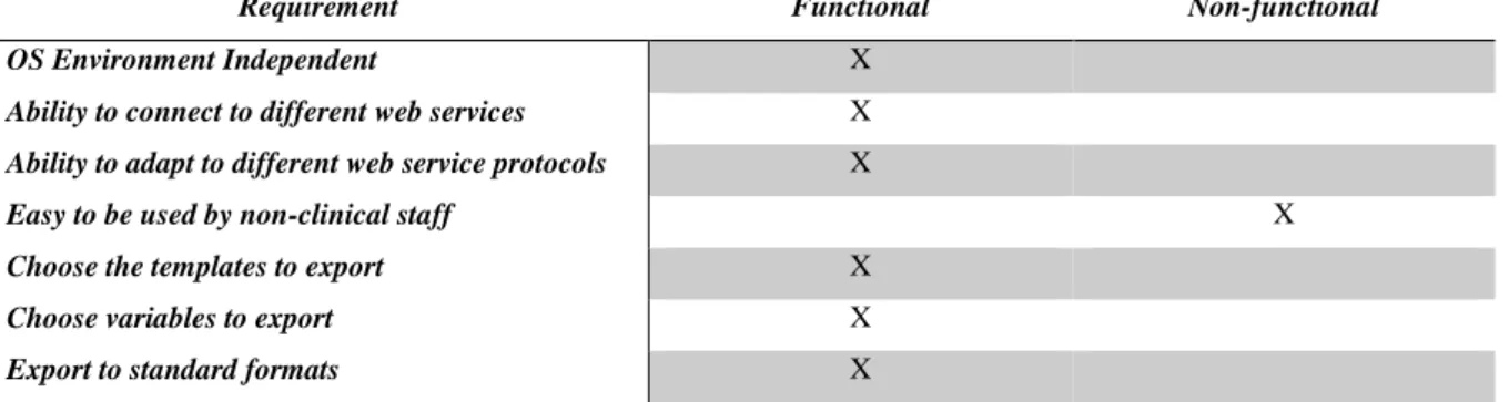
3.2 Functional and non-functional requirements ... 40
4 Architecture ... 43
4.1 Used technologies ... 43
4.2 openEHR export tool communication ... 43
5 Implementation... 45
5.1 Graphic user interface ... 49
5.2 Adopted methodology ... 49
6 Results ... 51
6.1 Tool operation ... 51
6.2 Tool exported data use ... 54
6.3 Tool application code ... 55
6.4 Comparative tests ... 59 6.5 Results summary ... 59 7 Discussion ... 61 7.1 General objective ... 61 7.2 Specific objectives ... 62 7.3 Limitations ... 62 7.4 Future work ... 62 7.5 Conclusion ... 63 8 References ... 65 9 Annexes ... 71
1
Achievements
Article submitted to the HCist 2014 International Conference on Health and Social Care Information Systems and Technologies and published on Procedia Technology
openEHR Translation Tool
2
3
1 Introduction
Nowadays, the need for information and the knowledge that it may provide are essential in the health care sector because, in essence, the practice of medicine is an information-driven strive. Whether to resource optimization, service evaluation or improving quality of service, systems generated information have yet unexplored potentialities.
However, the quality of data from where information is extracted is yet below the expected level and, thus leading to a situation in which the obtained knowledge is limited and often irrelevant or redundant. This is one of the main reasons that information systems who support physicians, health professionals, hospitals and primary care units fail to answer due to their base limitation: the quality of fed data, namely at the heath record level.
And what roots the lack of data quality? Usually, two reasons support this fact: non-investment in measures or infrastructures to improve data quality due to the fact that its economical return is not immediately visible and also the fact that data which is considered to be valuable to operational usage may not be suitable for medical research.
openEHR arose as a new instrument available to represent information and knowledge in health. It is a standard that comprises a set of electronic health care architecture specifications and establishes the base to the development of interoperable modular applications. As these specifications define the way clinical information concepts are organized by Information Services, obtaining semantic interoperability amongst different systems becomes possible. The openEHR standard is developed, revised and refined in a collaborative manner, sharing an international high quality and interoperable electronic health record vision.
1.1 Knowledge from data
In a time where is almost impossible to give a step without leaving a digital footprint, and if we transpose this idea to medicine, nearly every physician or medical staff activity produces data that is valuable for collection, review and management. The constantly growing volume of information will later give place to medical knowledge which will be used to provide the best patient health care possible.
For medical knowledge to increase, it requires valid data sets resulting from basic clinical-collected data to be used in research. This fact uncovers the utter importance of biomedical informatics, concerned with gathering, treating and optimally using information in healthcare
4
and biomedicine and why is it critical to the current and future practice of medicine by studying healthcare outcomes that result from this practice [1] [2].
Health information technology has become significantly important in medical research by implementing technologies like electronic health records, knowledge-management systems and clinical data storage, thus improving medical research and advancing outcomes research [3]. By outcomes research, we understand the comprehension of one or more health care practices and interventions end results [4]. These end results can influence decision-making processes towards resource management through better indicators such as cost-effectiveness or comparative effectiveness, since medical knowledge not only comprises “diseases and
diagnoses but also about the organization of health care and the procedures followed in the institutions through which health care is delivered”[5].
To achieve this, data collection must occur so it can be analyzed, treated and then forwarded to report findings. Therefore, patient or patient-related information generated during encounters or performed exams are one of the most important sources of information for knowledge extraction and clinical decision support systems.
In the healthcare environment, we have been observing an increasing progression of information systems which can support clinical research and several tasks, from medical encounters to patient information storage: EHR systems (to collect data in a structured format, reduce redundancy and identify intervention-eligible patients) [6], data mining tools (to predict patterns in patient conditions and their behaviors) [7], decision support systems (to provide clinicians with evaluations and recommendations to support clinical decision making) [8], computerized physician order entry systems (to automate the medication ordering process and implement legible and complete orders in a standardized form) [9], clinical data warehouses (to combine data from several sources to achieve conclusions otherwise impossible to achieve separately by means of business requirements analysis, data and architecture design) [10][11]. Such systems feed clinical information management platforms that have an important role in the improvement of healthcare.
1.1.1 Data Quality
As mentioned before, data is generated from the most various sources. However, none of this data is useful if not suitably stored. Data quality has an important part in this process and, contrary to what is often thought, is does not concern only data insertion errors or misspellings. In fact, the consequences of poor data quality can have an enormous impact on business and
5
organizations, leading to large costs due to several causes such as scattered or overlapping data, duplicated registries, inaccurate or unreliable information and incomplete or inconsistent data. Transposing this issue to the health sector, it is easy to understand its importance. Whether it is for research purposes or to resolve a structural question, data quality is vital to achieve proposed objectives and failure to assure it can have disastrous consequences, namely with the loss of human lives. Several tools exist to address these problems and with different application domains. Two examples of these tools which can be applied the health domain are Artkos [12] and ClueMaker [13]. While the first aims at the data integration instance-level conflict resolution and error localization through the application of a proprietary metamodel during the ETL process in a Data Warehouse for health applications and pension data (even though it’s an academic project), the latter has evolved for a commercial product and provides object identification and deduplication, removing duplicated copies of repeating data using clues as an input for a matching algorithm by means of rich expressions of the semantics of data [14]. 1.1.2 Interoperability
According to IEEE, interoperability is the “Ability of a system or a product to work with other systems or products without special effort on the part of the customer. Interoperability is made possible by the implementation of standards.” [15]. This definition implies other two notions:
technical interoperability; semantic interoperability.
By technical interoperability, we understand the exchange of data between systems, whichever means are used, and relies solely on the data exchange process. Concerning semantic interoperability, it relies on the ability of the destination system to use the exchanged data in a useful manner and applying the destination system business rules, thus sharing the same domain, interpretation, context, codes and identifiers between sender and destination systems. When technical and semantic interoperability is implemented, it is possible to move forward to achieve process interoperability, which is the conjunction of the first two with the fact of the human beings across a network can share a common understanding. In the healthcare sector these three types of interdependent interoperability are of particular importance, since information of an EHR in a specific healthcare unit must be accessible by health professionals or organizations in regions other than the one belonging to the patient’s residence area. One example of this interoperability is the epSOS project [16], aimed at the integration of several countries health data integration in a way that could be possible to access patient’s clinical
6
information even when outside of national territory. However, different levels of interoperability are found within European Union because of different views and barriers towards technological investment [17], even though it is widely agreed that semantic interoperability is the motor of life-long EHR's [18].
1.1.3 Decision Support Systems
It is a known fact that a bad or an uninformed decision can have a disastrous impact in an organization, whatever activity sector it belongs to. Due to high market competition and evolution, one decision can then mean the fall, maintenance or uprising in the rank of major players in a company’s market segment. One good example of poor decision making with a devastating result was the Blockbuster videogame and movie rental provider: by failing to observe and to adapt to the customers’ needs and market tendencies towards online movie renting rather than DVD or other physical support, it declared bankruptcy in 2010, after almost having the monopoly of movie and game rental in several countries.
Decision support systems (DSS) appeared to fill the gap between operational systems and the need to obtain information suitable for decision makers to opt for one of the several available hypothesis presented in the most grounded way. Since the majority of operational systems are not suited to the information needs, an adequate environment for storing and managing data creation became obligatory. However, to better understand the importance of DSS in an organizational context, some concepts must be apprehended first.
1.1.3.1 The decision-making process
The decision-making process for whatever problem involves several steps towards its solution in a successful manner or not. These steps are:
Situation identification and analysis; Alternatives development;
Alternatives comparison;
Classification of each alternative risk; Best alternative election;
Execution and evaluation.
Failing to build a decision based in the previous mentioned steps will lead to a poor decision support and, as a consequence, loss of outcome whether it may be financial or not.
7 1.1.3.2 Decision Characteristics
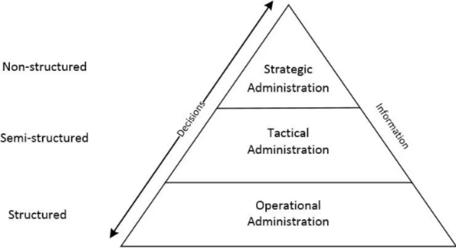
There are various kinds of decision, depending on the management level in which we are focusing. Figure 1 illustrates the relation between these two:
Figure 1 – Decision characteristics and management level relationship
As it can be observed, information is generated and used at operational, tactical and strategic administration levels to base every type of decision, which can be structured, semi-structured or unstructured, respectively.
By structured decisions, we understand the ones in which is possible to specify the procedure to follow. These decisions are typical of operational administration and an example can be the decision to perform an inventory. Operational systems are located at this level.
Semi-structured decisions are made at the tactical administration level and have some impact
along the time. Regarding to the procedure to follow, some steps can be previously known, but their influence in the final decision is not relevant. One example can be the decision to create a new institutional website or launching a new marketing campaign. Management information systems are located at this level.
Regarding the unstructured decisions, these are made at the strategic administration level and do not take in count the procedure to follow to implement them. These decisions have effect in the organization as a whole and one example can be the budget approval or a long term objective definition. Decision support systems are located at this level.
The organization decision-making is sequential in nature. Decisions are not isolated events and each of them has a relation to some other decision or situation. As it may appear as a ‘snap’, it is made only after long chain of developments and a series of related earlier decisions.
8
1.1.3.3 Decision support systems definition and positioning
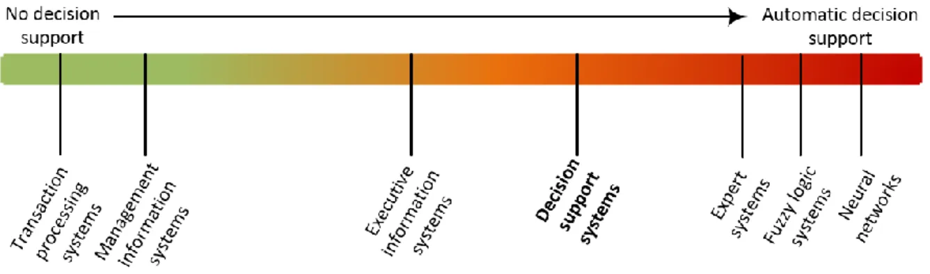
A decision support system is a complex system which allows access to the organization’s databases, problem modelling and simulation performing, amongst other features, in order to aid the decision maker to organize information and to assist in every step of the decision-making process [19]. It is mainly used in the resolution of complex and poorly structured problems and combines analytical models or techniques with traditional data processing functions, such as access and recovery of information. Figure 2 represents the positioning of decision support systems among other information systems.
Figure 2 – Decision support systems positioning
On the far left of the bar are located the transaction processing systems (TPS) and management information systems (MIS). These are projected for producing operational reports, based on routine operations with little or no integration and not oriented for decision support.
The far right side of the bar is where expert systems (ES) can be found. These systems use algorithms and advanced heuristics to replicate human logic to support decisions previously programmed to process, thus being excellent tools, but with a low flexibility level due to its narrow scope.
Somewhere in the middle of the diagram is the DSS and EIS (Executive Information Systems), which possess a high flexibility for data retrieval and analysis, providing a good decision support with specific tools that combine several viewpoints of data and allowing the decision maker to obtain valuable information.
Transposing this diagram to the reality of a company which sells a determined product, TPS and MIS can produce reports which show how many units have been sold and which has been the biggest buyer, the most profitable route of delivery or the lowest raw material cost supplier. However, a decision support system can produce reports combining information to achieve other conclusions, such as the most profitable product given the number of sold units with the
9
lowest raw material cost and with the most optimized route of delivery on a determined season of the year. This information can help the decision maker to whether invest in a big truck to maximize delivery route profit or to buy two smaller trucks to increase delivery flux over the second most profitable route.
Decision support systems can then have a wide range of application and can be found in different sectors of activity. Nevertheless, they are more valuable when used in an environment where dimension and lack of choices combine or simply no suitable data appears to be noticeable at first glance. One good example of this combination is the health sector: along with computerized physician order entry, decision support systems can decrease medication error rates and adverse drug events [20], while improving clinical practice. This is, however, a controversial matter, due to published studies stating that computerized physician order entry systems can also facilitate medication errors [21]. These two antagonistic views, despite of their motivations, uncover the need to improve these systems with everyone’s contribution.
1.2 Knowledge extraction systems
As previously stated, every day, an enormous amount of data is generated around the world and with the most diverse origins. Most managers consider that their workplace has too much information and don’t use it in decision making due to the information overload, storing it for later use and believe that the cost of information retrieval is higher than retrieved information real value. This situation leads to a situation where only a small amount of data is used due to its complexity and volume.
Being true that every generating system has its own method to bring out conclusions about its data, usually under the form of reports of listings, it is also true that organizations have more than one system or data source within their network or structure. Each of these data source can then be combined and/or analyzed to infer deductions otherwise impossible to obtain separately, which makes knowledge extraction techniques an extremely important tool for decision-making activities, supplying decision makers with concise and valuable information.
1.2.1 Data Warehousing and Data Mining
Data Warehousing and Data Mining concepts are tightly related, due to the fact that data mining algorithms are usually applied to data contained inside a data warehouse. To understand how these concepts relate with each other, it is important to first describe each of them separately.
10
1.2.1.1 Data Warehousing
A Data Warehouse (DW) belongs to the DSS category and according to Bill Inmon (2005), considered the father of the data warehouse concept, it is “a subject-oriented, integrated,
nonvolatile, and time-variant collection of data in support of management’s decisions.” [22].
In other words, a data warehouse is focused in a subject area (business process), combining cleansed data from different sources throughout a defined period of time in a way where mainly no data is updated or deleted. When data deletion or update is performed in the source systems, a new version is stored in the data warehouse expiring (but not deleting) the old version, thus enabling to find patterns in data that may help future decisions.
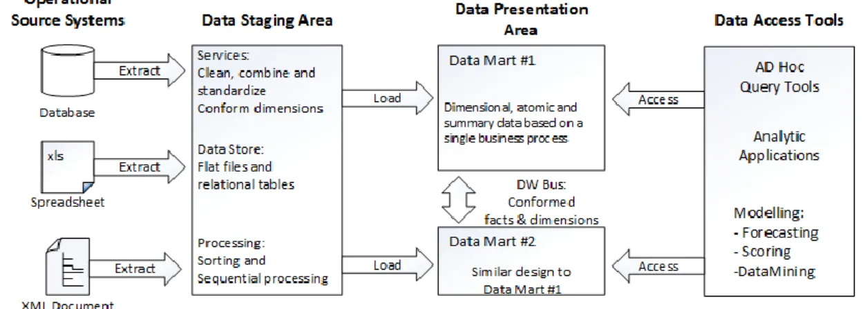
This collection of data flows within the data warehouse environment from the operational (production) environment through a complex process of extraction, transformation and loading of data (ETL). In this process, data is extracted from its sources to the Data Staging Area (DSA) where it is transformed (cleansed from incongruences, bad or missing values) using several techniques to minimize the possibility of later problems before being loaded into the Data Presentation Area (DPA), where one or more data marts are located. A data mart contains data from a single business process which, as we can deduct, will lead to the presence of more than one at this area. Data Access Tools (DAT) will then access these data marts to apply modelling techniques, such as data mining or to produce ad-hoc queries and reports [23]. This process is schematized in Figure 3, according to Ralph Kimball (2002).
Figure 3 – Data Warehouse basic elements
Queries are performed by data access tools against data marts and not in Data Staging Area, since this is where data is prepared to load. We can compare the DSA with a restaurant’s kitchen where meals are prepared for its customers so they can be served at the Data Presentation Area. Data Access Tools can range from ad hoc query tools for direct reporting (approx. 80 to 90 percent) to more complex tools for data mining, forecasting or other modelling applications
11
which may even feed their results back to operational systems, thus enriching source data for later extraction back into the data marts.
There are some important concepts within the data warehouse structure:
Time – time is always present, even if just implicitly, thus implementing the non-volatility characteristic of a data warehouse. So, it may or may not be present in a table form;
Fact table – This table stores the numerical measurements in an entire data mart, avoiding duplication across it and each row in this table represents a measure. Usually, its primary key is composed of foreign keys and it has a many-to-many relationship; Dimension table – Dimensional tables enclose the textual measurements or descriptors
and usually have a high number of columns, being related to fact tables;
Granularity – The level of granularity of a data warehouse is defined by its dimensions, as well as the measurements’ scope.
Data warehousing unveils the possibilities of derived data by combining different data sources in a multidimensional representation (data cube), which contains the facts (or cells), measures and attributes, thus implementing Line Analytical Processing (OLAP) by opposition to On-Line Transaction Processing (OLTP) present in an operational system [24]. The major differences between these two reside mostly in speed and the used schema for data storage. Table 1 table summarizes these differences by categories.
OLTP System OLAP System
Data Source Operational data Merged data from operational systems
Data Purpose Support business processes Support decision making, planning, and
forecasting
Speed Usually fast Speed is dependable of the stored data amount
Queries, Inserts and Updates Short and simple standard queries; Short and fast operations
Complex and long tailored queries; Long running batch jobs for data refresh Database design Highly normalized, usually 3NF;
Many tables
No normalization, usually star schema; Fewer tables
Space Consumed Relatively small Large consumption due to aggregates
Backup and Recovery Crucial for disaster recovery and
business continuity Not important for business continuity Table 1 – Differences between OLTP and OLAP Systems
Regarding data present in each of these systems within an organization, and due to its purpose, it can be said to be rather distinct. Even though OLAP systems originate in OLTP systems, the whole paradigm changes so it can be obtained a kind of data which can support decision
12
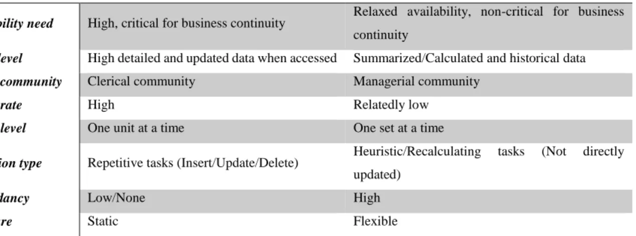
making. Primitive and derived data dissimilarities can then be better observed in Table 2 [25].
Primitive/Operational data Derived/DSS data
Availability need High, critical for business continuity Relaxed availability, non-critical for business continuity
Detail level High detailed and updated data when accessed Summarized/Calculated and historical data
Target community Clerical community Managerial community
Access rate High Relatedly low
Access level One unit at a time One set at a time
Operation type Repetitive tasks (Insert/Update/Delete) Heuristic/Recalculating tasks (Not directly updated)
Redundancy Low/None High
Structure Static Flexible
Table 2 – Operational data and DSS data differences
When implementing a data warehouse in a clinical context, the main reasons behind this decision are the need for administrators to have a broader view in terms of costs, personnel, bed allocation, billing, admission-discharge-transfer operations and expansion planning of the organization (hospital) or sector (in case of government institution), amongst others. It is known that clinical systems produce a high volume of data documenting patient care and several projects have been executed which have raised some difficulties and identified several problems in source systems to be solved, while developing techniques to optimize the ETL process and leading to successful but never-finished projects [25] [26].
Clinical Data Warehouses (CDW) are a specific implementation of the general data warehouse methodology and are central to evidence-based medicine by allowing access to healthcare providers to an information repository to which all have contributed. However, given the specificities of the health care, building a clinical data warehouse which serves manageability and investigation can be a challenging task [10].
1.2.1.2 Data Mining
Data Warehouses and other OLAP systems do not allow us to identify new groups, associations, rules or patterns in contained data, since OLAP systems are exploration-oriented, while data mining (DM) is knowledge-oriented. This has led to coupling OLAP with data mining to enable a next-generation systems towards KDD (Knowledge Discovery in Databases) with promising results, even though these two started by being considered different fields [27].
Data mining refers to the extraction of important and predictive information from a large amount of data or, as described by Mehmed Kantardzic (2011), “Data mining is a process of
13
discovering various models, summaries, and derived values from a given collection of data.”
[28]. It is widely accepted as an important mean to achieve the recognition of patterns or models in analyzed data through several algorithms and techniques such as neural networks, decision trees, genetic algorithms, nearest neighborhood or rule induction towards KDD [29].
Since its introduction in the late 1990’s, data mining has been applied in several fields, from finance to commerce or from health to business. With the dissemination and evolution of data mining systems as well as the processing capability power in the early 2000’s, new algorithms were introduced to perform outlier detection, web log and multimedia data matchmaking, bioinformatics mining, web mining and text mining, among others.
Integration of systems and the exponentiality of data generation by means of monitoring technologies and data streams, which are virtually impossible to store completely, led to the implementation of data sampling and the use of aggregations and, consequently, the emerging of parallel or distributed data warehousing concept through the growing use of XML technologies such as XML Schema-based data warehouse design, XML OLAP Cube in addition to already used standard data [30].
1.2.1.2.1 Data mining process and methodologies
Data mining projects are not easy to accomplish and many of them fail essentially due to the lack of vision (not knowing what information to bring out of data), incorrect, outdated or missing data, department bickering, legal restrictions, technical difficulties (several data formats) and poor interpretation. Since data mining is an iterative process, several steps were defined as essential, which are:
Present the problem and hypothesis formulation; Data gathering;
Data pre-processing (includes sub-tasks, such as data preparation and data reduction); Model construction (using the most appropriate techniques);
Model evaluation and interpretation.
For these steps to be accomplished successfully, a methodology must be followed. This ensures that, in every step of the project, it is possible to know what tasks were performed earlier, thus having an updated status regarding the overall project execution. Some data mining methodologies are described in light detail below and are based in previous stated step order, each of them with its changes [31].
14
PRMA methodology
PRMA stands for Preparation, Reduction, Modelization and Analysis. It was followed by Sholom Weiss and Nitin Indurkhya (1995) while describing a machine learning method for predicting the value of a real-valued function, given the values of multiple input variables [32] and essentially presents slight changes from the general steps:
Data origin business description; Data preparation;
Data reduction; Modelization; Analysis.
SCECMR Methodology
This methodology is a little more fragmented. It was developed by Usama Fayyad and is characterized by promoting two sub-steps of the general model and adding a third step, while renaming some to reflect the change:
Problem domain comprehension; Data Selection; Data Cleansing; Data Enrichment; Data Codification; Modelization; Reporting;
Model production implementation.
SEMMA Methodology
The SAS Institute (Statistical Analysis System Institute, Inc.) has developed this five-step methodology to conduct a data mining project [33]. Its name, as in with the previously presented methodologies, derives from the first letter of each of its steps designation:
Sample; Explore; Modify; Model; Assess.
15
CRISP-DM Methodology (CRoss-Industry Standard Process for Data Mining)
CRISP-DM is supported by the majority of the computational tools and one of the most used methodologies. It is well documented and implements the iterative and incremental features of the standard data mining process while running its own steps in a structured way, allowing for its revision in any stage [34]. An overview of the whole process can be found in Figure 4.
Figure 4 – The CRISP-DM methodology
As it can be observed, six stages are comprised in this methodology. The first stage focuses on understanding the project objective and transposing it onto an effective plan. The second stage is centered in understanding the gathered data, while identifying threats to its quality or possible hidden data subsets. The third stage involves all activities related to the construction of the data set which will be modeled. Next, on the fourth stage, several techniques will be applied according to its applicability to the raw dataset in a manner that they can be evaluated on the fifth stage to check for its compliance to the project objectives. If so, the sixth stage is achieved and the model is deployed.
Since it is a well-documented process, for every stage there is one or more sub-tasks resulting in a document containing important information for the next stages. Below, Table 3 presents each stage sub-tasks and resulting documents.
16
Stage Stage sub-tasks Stage resulting document(s)
Business understanding
Meeting for requisites understanding Meeting for business understanding Data source analysis
Model specification document Data selection process specification
Data understanding
Data selection process design Data combining
Data normalization Data tests
Technical specification regarding data selection process
Data quality document
Data preparation
Data selection for data mining process Data cleansing
Data codification
Technical specification about data document update
Modeling
Algorithm selection Test plan definition Model creation Model evaluation
Model evaluation document
Evaluation Real problem model evaluation Obtained results evaluation
Model evaluation document update Data mining process description document
Deployment
Obtained model deployment planning Process maintenance planning Model deployment
Data mining process description document final update
Obtained model results and its importance to business
Table 3 – CRISP-DM stage sub-tasks and resulting documents
For every data mining methodology, there are several common aspects. Whatever methodology is chosen, its process is iterative, giving place to a continuous feed along the process between stages and between iterations and the data mining process continues even after a solution is deployed. The process always starts with the problem/business understanding and all stages are similar between methodologies, while the data preparation are the ones that are more time and effort consuming.
1.2.1.2.2 Data mining techniques
Data mining methodologies are useful for organizing the whole process, but for each stage or aspect there are known problems and certain techniques to address them. For these and every other unexpected situations, the experience of the data miner is of the uttermost importance, since along the process several questions will be presented and the way they are dealt will dictate the success or failure of the data mining project.
Data preparation
17
set. This task is many times neglected when taught or in research over prediction methods but, in the real world, what happens is just the opposite.
When dealing with raw data sets, it is common to find missing values (such as measure errors or unavailable values), distortions, insertion errors or inadequate samples (which can generate outliers). So, some objectives at this point go through organizing data in a standard way to be processed by modelization software and choosing the best features (or variables) that lead to a better model performance, which normally involves data transformation.
Data organization
Computers have the ability to analyze many data in a standard way, but that same ability is limited by the description of original data. During this analysis, some data sets can be standardized, while others can present combinations or text for each feature. For learning or prediction methods to benefit from additional knowledge, it must be introduced at this point and each feature must be numerically coded. This coding can assume categorical values (eye color), discrete (qualitative) values, continuous (quantitative) values, periodical values or numerical values, which have an order or distance relation unlike categorical ones. However, a feature must me defined to prediction objective, thus promoting it to label.
Data transformation
In order to apply data mining techniques, there is always the need to transform original data. Even though transformations are not optimal and are mostly manually made, the human experience and knowledge are fundamental during feature selection and feature composition tasks.
Feature composition is related with data reduction, while feature selection focuses on normalization, smoothing and differences and ratios. By normalizing data, we understand a kind of transformation that reduces values to the same scale (e.g.: decimal), thus maintaining the values between an interval. Smoothing is applied when data detail will not be used by the data mining method, thus being a form of data reduction. Differences and ratios can contribute to learning methods by specifying a difference or ratio, leading to lower number of alternatives, while being possible to use with dependent or independent variables.
Missing data
18
depending on the amount of cases detected. If the missing value is the label value, the sample is discarded. However, if many samples have the label value empty, it will undoubtedly derail a whole project. Some solutions can be used, such as using a constant or the feature average, but it will never be the correct value.
Outliers
Outliers are sample values that do not fall within the scope of the remaining data model. They can be originated by a simple insertion error or, being plausible, resulting from a spurious data variation.
Determining outliers is a tricky task, because if a sample is considered an outlier and therefore erased, the model performance can be compromised. For instance, in credit card transactions analysis, outliers can be indicators of fraud. However, in the majority of applications this is not the case.
The most used techniques for outlier detection are statistic, distance or deviation-based.
Data reduction
We must never forget that when building a model, we are building one to apply to big data sets. So, the objective is to tune it with a sample data set before feeding it the whole one, which raises the question of what data can be selected without compromising result quality. Data reduction must then involve several analysis parameters, such as computational effort, learning speed, learning precision, model representation, model precision or complexity. These parameters are usually incompatible with each other and cannot be simultaneously improved. Some data reduction can be achieved by feature removal, case removal or value removal. Feature removal will enable higher precision and higher learning speed and can be accomplished by selecting a feature subgroup that has an identic performance to the whole group, by replacing the initial feature set with another one obtained from its composition or by feature ranking based on data consistency, information content, sample distance and feature statistic dependence.
Case removal is performed when the software that will be used or other techniques cannot handle the load. Usually, the most simple and used method is sampling in which the size depends on the feature number and problem complexity. This sampling can be random or systematic.
19
values are binned into discrete symbols. One good example is age categories (child, adolescent, adult, mid-aged and old): depending on the age value, it will belong to one of these discrete symbols. However, border values can be difficult to establish.
Data exploration
When exploring data, graphical representation greatly increases its meaning. Results nowadays can be represented in one, two, three, four or more dimensions and, according to Tufte (2007), graphical excellence “is that which gives to the viewer the greatest number of ideas in the
shortest time with the least ink in the smallest space” [35].
Some methods of visualization can assume the form of pie charts, bar charts, scatter plots or parallel coordinates, each of them with a proper use.
Additionally to graphical exploration, statistical methods can help to understand some aspects of a data set. Such methods include statistical measures for data location (mean, median or mode) and data dispersion (variance or standard deviation). Other measures can relate two or more features to determine their dependency or relation, like covariance or correlation matrices.
Learning from data
Data mining approaches are based in human learning capabilities and computational learning is made from data. It consists of two main phases:
Estimating unknown dependencies in the system;
Using estimated dependencies to predict new outputs for later system data feed.
These phases correspond to the two classical types of inference (induction and deduction), which can be observed in Figure 5.
20
In the inference process, a training data set provides induction to the model estimation that, when fed with a priori knowledge (usually human-driven) can make deductions and predict outputs. Estimating only one model implies a global function learning for all input values, which generates a problem when the objective is to only deduct estimates for some values. So, when estimating a function without building a global model, transduction is used.
Model estimation process can be described, formalized and implemented using different learning methods. These learning methods are algorithms which estimate an unknown mapping or dependency between entries and outputs of a system from a data set and, when precisely estimated, it can be used to predict outputs given its inputs.
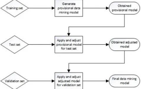
Within the data mining methods, we can catalogue them as supervised or unsupervised. Supervised methods are used to estimate a dependency from known input-output data while in unsupervised methods only the input data are known and the algorithm searches for patterns among all variables. The majority of data mining methods is supervised, which means they preprocess data from a training set so the algorithm can learn the association between the variable values and the predictor variables. However, the model obtained from this training set must be validated so it won’t act prejudicially when applied to the data to be classified. This provisional model is applied to a test set where the target variable values were hidden to observe how the model behaves. After the necessary adjustments to decrease error rate, the obtained model is then applied to a validation set again with the target variable values hidden where some more adjustments are made to minimize error rate. The resulting model is then ready to apply to the final data set to be evaluated. The whole view of this process is shown in Figure 6.
21
The accuracy values on the test set and on the validation set will not be as high as the ones on the training set, due to overfitting. Overfitting is the violation of the principle of parsimony, in which is stated that a model or procedure must contain all that is necessary for the modelling, but nothing more [36]. When overfitting occurs, certain idiosyncratic trends or structures are computed, which may lead to erroneous interpretation.
Between model complexity and generalizability, a balance must be achieved in order to obtain a model which can be reliable. When increased, model complexity will result in a more accurate model in the training set, but a higher error rate in provisional and test sets.
There are no guidance lines on how to perform data splitting to obtain the training or test sets, even though it is known that a small training set will result in a low robust model and with a weak generalization capability and that a small test set will lead to a low confidence in the generalization error. However, there are some techniques for addressing these issues, being all the most used ones based in the resampling concept:
Resubstitution – all samples are used for training and test sets. It is the simplest method, but also not common to use in real data mining applications;
Holdout – Half or two thirds of data are used for the training set and the remaining are used for the test set. Because each set samples are independent, the generalization error is pessimist but, repeating the process with different training and test set samples randomly selected will improve the estimated model;
Leave-one-out – the resulting model is obtained from using n-1 samples for training and evaluated with the remaining ones and then repeated n times with different training sets of size n-1. This approach demands high computational resources, since it is necessary to build and compare many models;
Cross-validation – This is a mix of the holdout and leave-one-out methods. Data is divided in P subsets, all of equal size. P-1 subsets are used for training and the remaining ones are used for test sets. This is the most used method;
Bootstrap – In its simplest form, instead of repeatedly analyzing data subsets, random subsampling with complete sample substitution is analyzed. This allows to generate “fake” data sets with the same size of the original data set, which is useful when working with data sets that have a low number of samples.
Model evaluation
22
error). Such evaluations are performed using metrics like Mean Square Error, Root Mean Square Error or Non-Dimensional Error Index for regression problems or hypothesis evaluation for classification problems. Regression problems are related with the prediction of a result based on two or more variables whilst classification problems point a class where a sample should be placed.
In a classification problem, the error rate is:
𝐸𝑟𝑟𝑜𝑟 𝑟𝑎𝑡𝑒 = 𝑁𝑢𝑚𝑏𝑒𝑟 𝑜𝑓 𝑒𝑟𝑟𝑜𝑟𝑠 𝑛𝑢𝑚𝑏𝑒𝑟 𝑜𝑓 𝑐𝑎𝑠𝑒𝑠
This logically means that the accuracy of a model is obtained by:
1 − 𝐸𝑟𝑟𝑜𝑟 𝑟𝑎𝑡𝑒
For hypothesis evaluation, each case (or sample) receives a “verdict”. In this perspective, it can be found to be a true positive (TP), true negative (TN), false positive (FP) or false negative (FN). As it can be deducted, a true positive or true negative is a sample correctly classified respectively as positive or negative, while a false positive or false negative is a sample classified as positive or negative when in reality it was found to be otherwise.
When measuring a model precision or sensibility, the percentage or correctly predicted items in a given class can be obtained by:
𝑃 = 𝑇𝑃
𝑇𝑃 + 𝐹𝑃
For recall or specificity model measuring, the percentage of correctly classified items in a given class is obtained by:
𝑅 = 𝑇𝑃
𝑇𝑃 + 𝐹𝑁
Model evaluation is of great importance due to the fact that a balanced model will be possible to apply to the real dataset and perform in the most optimized way, whatever its size. It is virtually impossible to build a flawless model, but it is very easy to build one that has a high generalization degree and also a high error rate. The keyword is, therefore, balance.
23
1.2.1.2.3 Data mining algorithms
To build a model, it is necessary not only to apply the right techniques but also the right algorithms to the data set in a way that information can be extracted. There is a myriad of available algorithms which can be used with this objective, each of them with their advantages and disadvantages. The most used ones are described below, even though there are many more (including variants) which can be applied.
Bayes Classifier
The Bayes Classifier has its roots in the Bayes theorem, which can be observed below. This allows for the classifier to add external information in the data analysis process with an a priori probability and also with an a posteriori probability.
𝑃(𝐻|𝑋) =𝑃(𝑋|𝐻)𝑃(𝐻) 𝑃(𝑋)
The X symbolizes the sample intended to be classified, while H represents the hypothesis to be tested. P(H|X) is the probability of H to be true, given observation X (a posteriori probability) and P(H) is the probability of H to be true (a priori probability).
In theory, the Bayes Classifier has the lowest classification error when compared with other classification algorithms. However, that not always is true due to uncertainty regarding some assumptions about features and conditional independence of classes.
Linear Regression
The objective of the regression analysis is to determine the relation between the output variable (Y) and one or several input variables (X1, X2,…, Xn). Since the measurement of the output
value can be expensive, it is more affordable to measure de input values and establish the relationship between them in a way that it is possible to control the output.
Decision Trees
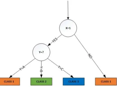
Decision trees are widely used in the real world, especially in classification problems. The objective is to create a classification model in which is possible to predict the class of a new sample.
24
attributes are tested, while branches and leaves represent the possible values attributes can take and the classes’ tags, respectively. The path between the root and one leave expresses a decision rule. Figure 7 presents an example of a decision tree.
Figure 7 – Decision tree example
One of the most used algorithms within decision trees is the ID3 algorithm. It starts by choosing one attribute to partition samples and then applying the same method to the partitioned samples recursively. Each branch of the tree represents one decision rule and the algorithm relies on the concepts of entropy and information gain to generate them. These concepts derive from the Claude Shannon’s Information Theory [37].
Entropy can be defined, in information theory, as the measure of uncertainty regarding a random variable (or sample) and the average information lost. The ID3 algorithm aims at the entropy minimization by minimizing the number of tests needed to classify a sample. This can be translated in the following formula:
𝐸𝑛𝑡𝑟𝑜𝑝𝑦 (𝑆) = − ∑ 𝑝i 𝑛 𝑖=1 ∙ log2(𝑝i) Being that 𝑝i= 𝑛𝑢𝑚𝑏𝑒𝑟 𝑜𝑓 𝑟𝑒𝑔𝑖𝑠𝑡𝑟𝑖𝑒𝑠 𝑖𝑛 𝑐𝑙𝑎𝑠𝑠 i 𝑡𝑜𝑡𝑎𝑙 𝑛𝑢𝑚𝑏𝑒𝑟 𝑜𝑓 𝑟𝑒𝑔𝑖𝑠𝑡𝑟𝑖𝑒𝑠
The information gain concept, which consists in minimizing the needed information to classify a sample in the resulting sub tree, is applied by the ID3 algorithm recurring to the following formula:
25
𝐺𝑎𝑖𝑛 (𝑆, 𝐴) = 𝐸𝑛𝑡𝑟𝑜𝑝𝑦(𝑆) − ∑ 𝑝i 𝑚
𝑖=1
∙ 𝐸𝑛𝑡𝑟𝑜𝑝𝑦(𝑆i)
Attribute selection for a node is based on the assumption that the tree’s complexity is related with the amount of information contained in an attribute’s value, thus leading to the objective of minimizing the number of tests to classify a sample from a given dataset.
However, the ID3 algorithm has a high sensitivity to features with a high number of different values, such as social security numbers. This situation will lead to low entropy values, unless there is a way to circumvent it. Since ID3 gives preference to high ramification factor, C4.5 algorithm uses the ratio between information gain and entropy from the sample set. This can be represented by 𝐺𝑎𝑖𝑛𝑅𝑎𝑡𝑖𝑜(𝑝, 𝑇) = 𝐺𝑎𝑖𝑛(𝑝, 𝑇) 𝑆𝑝𝑙𝑖𝑡𝐼𝑛𝑓𝑜(𝑝, 𝑇) Where SplitInfo is 𝑆𝑝𝑙𝑖𝑡𝐼𝑛𝑓𝑜(𝑝, 𝑡𝑒𝑠𝑡) = − ∑ 𝑃′ 𝑛 𝑗=1 (𝑗 𝑝) ∙ log (𝑃′ ( 𝑗 𝑝))
By applying the gain ratio to the data set being tested for the node, C4.5 chooses the best fitted attribute to split the set based on the normalized information gain. In addition, C4.5 allows to work with missing and numerical value attributes, as well as to perform the tree pruning by discarding branches which does not contribute to error reduction in the classification [38]. There are several advantages in using decision trees such as the possibility to work with continuous values as well as symbolic values, the ability to generate understandable rules, the construction of interpretable models, the clear designation of the most important features contributing to prediction and the fact of being light from the computational point of view, among others. However, there are some disadvantages which restrain its wider use. Namely, the size of the tree has a great influence on its accuracy due to the fact that when having a high number of splitting characteristics, the classification algorithm tends to increase the branch number, rendering the extracted decision rule useless or highly difficult to understand. Other limiting characteristic is that most of the algorithms demand discrete values as target attributes in order to be applied, which excludes most induction algorithms which can be used [39]. In conclusion, decision trees allow to generate decision rules during which generalization is applied and the rule set is compact. This process implies ordering the resulting rules, being
26
necessary to state a class to allocate the undefined samples by the resulting rules.
Association Rules
This is the most common way to find local patterns in non-supervised systems with the objective of finding interesting rules which are previously unknown. However, information overload needs to be avoided in order to keep data analysis as smooth and quick as possible [28].
Three types of association rules can be obtained from applying algorithms to a specific dataset: the useful rule (which can be explained in an intuitive way), the trivial rule (which does not add any value to an empiric experience) and the inexplicable rule (which does not have a plausible explanation).
One of the most used examples for association rules is the market basket analysis. In this analysis, the shopping cart (market basket) content is examined in order to find items which are repeated in other shopping carts (itemsets) and can contribute to define item localization in stores or to provide client-oriented advertising based on shopping habits. Nevertheless, it can be applied to other domains, such as business or research. For instance, to predict service degradation during utilization peaks in diverse times of the year on a cell network, detecting insurance fraud or even in studying a new drug side effect. Several difficulties arise here, namely the high number of baskets to examine, the exponential frequent itemsets in relation to different items and the need for scalable algorithms in order to increase linear complexity par opposition to exponential complexity due to computational resources limitation.
To find frequent itemsets, its support must be higher than a certain value and by support we understand the percentage of transactions that contain that same itemset. In addition, an itemset that contains x items is called an x-itemset [39].
The Apriori Algorithm is the reference algorithm to discover association rules within data. It was first presented in 1994 by Rakesh Agrawal and Ramakrishnan Srikant and it is composed by two phases. In the first phase, it starts by generating candidates and then it performs the counting and selection of the obtained candidates. In the second phase, the algorithm generates the association rules. The pseudo code for algorithm can be found in Figure 8.
27 Figure 8 – Apriori Algorithm pseudo code
Like any other algorithm, Apriori has some advantages and disadvantages. Amongst the advantages, we can list the ease of data interpretation, the ease of understanding and the possibility to produce results without certainty or expectation. However, the exponential growth complexity along with the problem dimension, the poorly defined detail level and the problems arisen with products (items) which have a low degree of appearance (Market Basket Analysis) are the main disadvantages of this algorithm.
Clustering
When analyzing samples, sometimes it is useful to group them in classes by resemblance. Clustering is a set of methodologies aimed at automating records association by segmenting a whole data set in groups based on similarities for better interpretation and deeper analysis, where patterns that may exist in data are unknown, thus not existing predefined classes. This record organization is not classification-oriented mainly because there is no target variable to predict or estimate and, unlike association rules process, clustering belongs to the unsupervised learning category. One cluster aggregates several samples with similar characteristics, being that these same samples are distinct from others belonging to other clusters.
Typical applications for clustering are the initial data relation discovery, pre-processing stage for other algorithms, pattern recognition, geographical data analysis, image processing, financial data analysis or document classification in a web context.
Several algorithms can be invoked, each of them with its own approach. For illustrative purposes, only the K-means algorithm will be described, which is one of the most used and is positioning-based. However, there are other algorithms that can be used, depending on the desired objective. Other approaches comprise hierarchy (BIRCH, CURE), density-based
28
(DBSCAN, OPTICS, CLIQUE), grid-based (STING, WaveCluster) or model-based (statistical approach, AI, Soft Computing).
K-means algorithm follows a five step procedure to achieve its objective. In the first step, the number of clusters (groups) is defined (K). The next step is to randomly calculate the cluster initial center (or seed) so it can be possible to associate each sample to its nearest seed in the third step. In step four, a new center for each cluster is estimated and, in the fifth step, a repetition of steps three and four are performed until the algorithm converges.
It is important to refer that K-means can only be used with numerical (and preferably normalized variables). Also, the partitioning result depends of the prototype initialization, which make it necessary to avoid circumstances where the algorithm can be “stuck” in a local minimum. One possible alternative is to run the algorithm several times and with different initializations in order to achieve an optimal global positioning clustering.
Amongst its advantages, the K-means algorithm is a simple and easy one to understand and its samples are automatically associated to clusters. On the other hand, the need to define the initial cluster number along with the obligation that each sample belongs to a cluster makes this algorithm too sensitive to outliers, which can lead to problems when dealing with different size, density or form clusters [28][40].
1.3 openEHR
The electronic health record is one of the root components in health. What started by an initiative to evolve from paper records to digital records soon became a source of information on which bases great part of today’s medical research.
It is a known fact that standards exist in many areas, and the healthcare sector is no exception. According to International Organization for Standardization (ISO), a standard can be defined as “a document that provides requirements, specifications, guidelines or characteristics that
can be used consistently to ensure that materials, products, processes and services are fit for their purpose” [41].
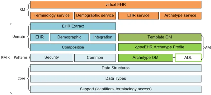
openEHR is an “open standard specification that describes the management, storage, retrieval
and exchange of data in Electronic Health Record” [42]. It first appeared in 1992 inserted in
the GEHR/openEHR European project. Later, Australia invested in the initiative, in the meantime renamed from Good European Health Record to Good Electronic Health Record. Currently maintained by the non-profit openEHR Foundation [43], an international and online community to promote electronic health records of high quality supporting the need of patients