q
-distributions in complex systems: a brief review
S. Picoli Jr., R. S. Mendes, L. C. Malacarne and R. P. B. Santos
Departamento de F´ısica and National Institute of Science and Technology for Complex Systems, Universidade Estadual de Maring´a, Avenida Colombo 5790,
87020-900 Maring´a, PR, Brazil
(Received on 26 March, 2009)
The nonextensive statistical mechanics proposed by Tsallis is today an intense and growing research field. Probability distributions which emerges from the nonextensive formalism (q-distributions) have been applied to an impressive variety of problems. In particular, the role ofq-distributions in the interdisciplinary field of complex systems has been expanding. Here, we make a brief review ofq-exponential,q-Gaussian andq-Weibull distributions focusing some of their basic properties and recent applications. The richness of systems analyzed may indicate future directions in this field.
Keywords:q-exponential,q-Gaussian,q-Weibull, Nonextensive statistics
1. INTRODUCTION
Common characteristics of complex systems include long-range correlations, multifractality and non-Gaussian distribu-tions with asymptotic power law behavior. Typically, such systems are not well described by approaches based on the usual statistical mechanics. In this scenario, a new formalism capable of providing a better description of complex systems is welcome. This is the case of the generalized (nonextensive) statistical mechanics proposed by Tsallis - nowadays, an in-tense and growing research field[1–4].
Concepts related with nonextensive statistical mechanics have found applications in a variety of disciplines including physics, chemistry, biology, mathematics, geography, eco-nomics, medicine, informatics, linguistics among others[5– 7]. Probability distributions which emerge from the nonex-tensive formalism - also calledq-distributions - have been ap-plied to an impressive variety of problems in diverse research areas including the interdisciplinary field of complex systems. In the present work we focus onq-exponential,q-Gaussian andq-Weibull distributions. We summarized some of their basic properties and provide useful references of recent ap-plications. The richness of systems analyzed may indicate future directions in this research line.
2. q-EXPONENTIAL DISTRIBUTION
The q-exponential distribution is given by the probability density function (pdf)
pqe(x) =p0
1−(1−q) x x0
1/(1−q)
(1)
for 1−(1−q)x/x0≥0. Ifp0= (2−q)/x0, eq. (1) is
normal-ized.
In the limit q→1, eq. (1) recovers the usual exponen-tial distribution in the same way in which theq-exponential function, defined ase−qx≡[1−(1−q)x]1/(1−q), recovers
ex-ponential function in the limitq→1 (e−1x≡e−x). Ifq<1, eq. (1) has a finite value for any finite real value of x since, by definition,pqe(x) =0 for 1−(1−q)x/a<0. Ifq>1, eq.
(1) exhibits power law asymptotic behavior,
pqe(x)∼x−1/(q−1). (2)
0 1 2 3 4
0,0 0,5 1,0
q=2,5 q=1,5 q=1,0 q=0,5
pqe
(x
)
x
(a)
0,1 1 10 100
10-3
10-1
q=2,5 q=1,5 q=1,0 q=0,5 pqe
(x
)
x
(b)
0 1 2 3
-2 -1 0
x0=2.5 x0=1.5 x
0=1.0 x0=0.5
lnq pqe
(x
)
x (c)
FIG. 1:q-exponential distribution. a) Plot ofpqe(x)versusx, with
p0=x0=1 and typical values ofq. b) Log-log plot of the curves in
a). c) lnqpqe(x)versusxforp0=1 and typical values ofx0.
Note also thatpqe(x)≃1+xfor smallx, independently of the
q value. Figures 1a and 1b showpqe(x)versusxfor typical
values ofq.
100 102 104 106 101
103
R
(P
)
P USA
(a)
0,0 5,0x10⁶
1,0x10⁷
0 1
lnq
’
R
(P
)
P USA
(b)
103
104
105
106
107
10-1
101 103
R
(P
)
P
(c)
Brazil
0,0 5,0x10⁶
1,0x10⁷
0,0 0,5 1,0 1,5
lnq
’
R
(P
)
P (d)
Brazil
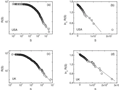
FIG. 2:Population of cities.a) Empirical cdfR(P), wherePis the population of USA cities. The solid line is aq-exponential, given by eq. (3), withq′=1.7 (q≃1.4),x′0=21,250 andc′=2,919. b) lnq′R(P)versusP, withq′=1.7, for the same data shown in (a). The solid line
is a linear fit to the data. c) Empirical cdfR(P), wherePis the population of Brazilian cities. The solid line is aq-exponential, given by eq. (3), withq′=1.7 (q≃1.4),x′0=7,073 andc′=6,968. d) lnq′R(P)versusP, withq′=1.7, for the same data shown in (c). The solid line is
a linear fit to the data.
103
104
105
106
107
101
103
R
(S
)
S
(a)
USA
0 1x10⁷
2x10⁷
0,4 0,8 1,2 1,6
lnq
’
R
(S
)
S
(b)
USA
103
104
105
106
107
101
103
R
(S
)
S
(c)
UK
0 1x10⁶
2x10⁶
3x10⁶
0,4 0,8 1,2 1,6
lnq
’
R
(S
)
S
(d)
UK
FIG. 3:Circulation of magazines. a) Empirical cdfR(S), whereSis the circulation of 570 USA magazines in 2004. The solid line is a
q-exponential, given by eq. (3), withq′=1.65 (q≃1.4),x′0=255,204 andc′=594. b) lnq′R(S)versusS, withq′=1.65, for the same data
shown in (a). The solid line is a linear fit to the data. c) Empirical cdfR(S), whereSis the circulation of 727 UK magazines in 2005. The solid line is aq-exponential, given by eq. (3), withq′=1.65 (q≃1.4),x′0=37,493 andc′=860. b) lnq′R(S)versusS, withq′=1.65, for
the same data shown in (c). The solid line is a linear fit to the data.
The cumulative distribution function (cdf) associated to eq. (1) is given by
Rqe(x) =
Z ∞
x
pqe(y)dy
= p′0
1−(1−q′) x x′0
1/(1−q′)
, (3)
defined forq<2, withq′=1/(2−q),x′0=x0/(2−q)and
p′0=p0x0/(2−q). Observe thatRqe(x)andpqe(x)exhibit the
same mathematical form.
It is possible to visualize q-exponential distributions as straight lines in graphs with appropriate scales. Applying the q-logarithm function, defined as lnqx≡[x(1−q)−1]/(1−q),
with ln1x≡ln(x), in both sides of eq. (1), we have
lnqpqe(x) =lnqp0−[1+ (1−q)lnqp0]
x x0
A similar result holds forRqe(x). Figure 1c shows lnqpqe(x)
versusxfor typical values ofx0.
The q-exponential function given by eq. (1) has been employed in a growing number of theoretical and empiri-cal works on a large variety of themes. Examples include scale-free networks[10–14], dynamical systems[15–27], al-gebraic structures[28–31] among other topics in statistical physcics[32–36].
As specific examples of q-exponential distributions in complex systems, let us consider results on population of cities[37] and circulation of magazines[38]. Figure 2 shows the cumulative distribution of the population of cities in the USA and Brazil. Figure 3 shows the cumulative distribution of circulation of magazines in the USA and UK. In both cases - population of cities and circulation of magazines - the em-pirical data are consistent with aq-exponential distribution, withq≃1.4.
q-exponential distributions have also been applied in the empirical study of stock markets[39–42], DNA sequences[43], family names[44], human behavior[45–47], geomagnetic records[48, 49], train delays[50], reaction kinetics[51], air networks[52], hydrological phenomena[53], fossil register[54], basketball[55], earthquakes[56–58], world track records[59], voting processes[60], internet[61], individual success[62], citations of scientific papers[63, 64], football[65], linguistics[66, 67] and solar neutrinos[68, 69].
3. q-GAUSSIAN DISTRIBUTION
Theq-Gaussian distribution is specified by the pdf
pqg(x) =p0
"
1−(1−q) x
x0
2#1/(1−q)
, (5)
for 1−(1−q)(x/x0)2≥0 and pqg(x) =0 otherwise. It is
normalized ifp0= (2/x0)
p
(q−1)/π Γ[1/(q−1)]/Γ[1/(q− 1)−1/2]. In addition, eq. (5) presents unit variance ifx20= 5−3q, withq<5/3.
In the limitq→1, eq. (5) recovers the usual Gaussian dis-tribution, soq6=1 indicates a departure from Gaussian statis-tics. Forq>1, the tails ofq-Gaussian decrease as power laws,
pqg(|x|)∼ |x|−2/(q−1). (6)
Figures 4a and 4b showpqg(x)for typical values ofq.
Applying theq-logarithm function in both sides of eq. (5), we have
lnqpqg(x) =lnqp0−[1+ (1−q)lnqp0]
x
x0
2
. (7)
Figure 4c shows lnqpqg(x)versusx2for typical values ofx0.
Recent works have been focused on the study of mathe-matical properties of q-Gaussian functions[70–78], includ-ing methods for generatinclud-ing random numbers which fol-low q-Gaussian distributions[79, 80]. q-Gaussians have been employed in the study of a wide range of themes in-cluding probabilistic models[81, 82], stellar plasmas[83], porous-medium equation[84], Bose-condensed gases[85–87],
-4 -2 0 2 4
0 2 4
q=1.7 q=1.5 q=1.3 q=1.0
pqg
(x
)
x
(a)
-8 -4 0 4 8
0,01 0,1 1 10
q=1.7 q=1.5 q=1.3 q=1.0
pqg
(x
)
x
(b)
0 4 8
-6 -3 0
x0=1.7 x0=1.5 x0=1.3 x0=1.0 lnq
pq
g
(x
)
x2
(c)
FIG. 4: q-Gaussian distribution. a) Plot ofpqg(x)versusx, with
p0=x0=1, for typical values ofq. Some curves were vertically
shifted for a better visualization. b) The same curves shown in a), but for mono-log scale. Some curves were also shifted . c) lnqpqg(x)
versusx2forp0=1 and typical values ofx0.
dynamical systems[88–90], polymeric networks[91], small-world networks[92], fingering processes[93], processes with stochastic volatility[94, 95] and nonlinear diffusion[96, 97].
In order to illustrate a recent application ofq-Gaussian dis-tributions in complex systems, we mention here results on the dynamics of earthquakes[98]. Figure 5 shows the distribution of energy differences between successive earthquakes at the San Andreas Fault. The empirical data is consistent with a q-Gaussian distribution, withq=1.75.
Other recent applications of q-Gaussian distribution in-clude stock markets[99–107], DNA molecules[108], the solar wind[109–111], galaxies[112], optical lattices[113], cellular aggregates[114] and the atmosphere[115].
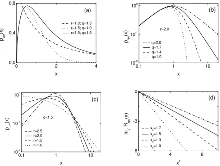
4. q-WEIBULL DISTRIBUTION
Theq-Weibull distribution is given by the pdf
pqw(x) =p0
rxr−1
xr0
1−(1−q) x
x0
r1/(1−q)
, (8)
for 1−(1−q)(x/x0)r≥0 andpqw(x) =0 otherwise. Eq. (8)
is normalized ifp0=2−q.
re--40 -20 0 20 40 10-5
10-3 10-1
P
(Z
)
Z
(a)
0 10 20 30
-400 -200 0
lnq
p
(Z
)
Z2
(b)
FIG. 5:Earthquakes. a) Empirical pdfP(Z), whereZ=E(t+1)−E(t)is the energy difference between successive earthquakes at the San Andreas Fault in the period 1966-2006. The solid line is aq-Gaussian, given by eq. (5), withq=1.75,x0=0.25 andp0=1.63. b) lnqP(Z)
versusZ2, withq=1.75, for small values ofZ. The solid line is a linear fit to the data.
0 2 4
0,0 0,4 0,8
r=1.0; q=1.5 r=1.5; q=1.0 r=1.5; q=1.5
pqw
(x
)
x
(a)
0,1 1 10
10-2
10-1
100
r=2.0
q=2.0 q=1.7 q=1.4 q=1.0
pqw
(x
)
x
(b)
0,1 1 10
10-2
10-1
100
q=1.5
r=2.5 r=2.0 r=1.5 r=1.0
pqw
(x
)
x
(c)
0 4 8
-6 -3 0
x0=1.7 x0=1.5 x0=1.3 x
0=1.0
lnq
’
R
q
w
(x
)
xr
(d)
FIG. 6:q-Weibull distribution. a) Plot ofpqw(x)versusx, withp0=x0=1, and typical values ofqandr. b) Log-log plot ofpqw(x)versus
x, withp0=x0=1,r=2 and typical values ofq. c) a) Log-log plot ofpqw(x)versusx, withp0=x0=1,q=1.5 and typical values ofr. d)
lnq′Rqw(x)versusxrforp′0=1 and typical values ofx0.
spectively. Ifq<1,pqw(x)has a finite limit sincepqw(x) =0
for 1−(1−q)(x/x0)r<0. Ifq>1,pqw(x)exhibits power law
behavior both for small and large values ofx. More specifi-cally,
pqw(x)∼x−ξ, (9)
withξ= (1−r)for smallxandξ=r[(2−q)/(q−1)] +1 for largex. Figures 6a, 6b and 6c show pqw(x)versusxfor
typical values ofqandr.
The cdf associated topqw(x)is given by
Rqw(x) =p′0
1−(1−q′)
x x′0
r1/(1−q′)
, (10)
withq′=1/(2−q),(x′0)r=xr
0/(2−q)andp0′ =p0/(2−q).
Applying theq-logarithm function in both sides of the cdf Rqw, we have
lnq′Rqw(x) =lnq′p′0−[1+ (1−q)lnq′p′0] x
x0
r
. (11)
Figure 6c shows lnq′RqW(x)versusxrfor typical values ofx0.
If pqw(x)is normalized (p0=2−q), Eq. (11) reduces to
lnq′Rqw(x) =−(x/x0)r. In this case,
ln[−lnq′(Rqw(x))] =rlnx−rlnx0. (12)
As specific example ofq-Weibull distribution in complex systems, we now consider results on citations in scientific journals[116]. Figure 7 shows the distribution of the impact factor of scientific journals in comparison with aq-Weibull curve. The empirical data is consistent with aq-Weibull dis-tribution, withq=1.45 andr=1.50.
0,01 0,1 1 10 100 10-3
10-1
p
(F
)
F
(a)
0 100 200 300
0,6 0,9 1,2
lnq
’
R
(F
)
Fr
(b)
FIG. 7: Citations in scientific journals. a) Empirical pdf p(F), whereFis the 2004 impact factor for 5912 scientific journals. The solid line is aq-Weibull distribution, given by eq. (8), withr=1.5,
q=1.45,x0=0.74 andp0=0.58. b) lnq′R(F)versusFr, with
q′=1.82 (q=1.45) andr=1.5. The solid line is a linear fit to the data.
5. BASIS FORq-DISTRIBUTIONS
¿From the viewpoint of the principle of the maximum en-tropy, someqdistributions optimizes generalized entropies -more general entropic measures than the standard Boltzmann-Gibbs entropy. A striking example is theq-entropy proposed by Tsallis[1]
Sq=
1−∑Wi=1p q i
q−1 , (13)
whereW is the total number of microstates of the system,pi
are the occupation probabilities andqis a real parameter. The standard Boltzmann-Gibbs entropy is recovered in the limit q→1.
The maximization ofSqsubject to specific constraints
gen-erates occupation probabilities following aq-exponential dis-tribution. Theq-exponential optimizes other generalized tropic measures such as the Renyi and normalized Tsallis en-tropies. However, only Tsallis entropy can provide an appro-priate basis for theq-exponential distribution since it presents several properties essential for an entropy[122, 123]. Chang-ing the constraints, the maximization ofSqalso generates
oc-cupation probabilities following aq-Gaussian distribution. Formally, q-distributions can arise when the exponen-tial function of the original distribution is replaced by a
q-exponential function. For example, this basic procedure ap-plied in standard exponential, Gaussian and Weibull distri-butions leads to q-exponential, q-Gaussian and q-Weibull, respectively[55]. This viewpoint suggests the consideration of other q-distributions which could be obtained by simply replacing its exponential function by aq-exponential one.
q-distributions can also emerge from compound distributions[124]
pq(x) =
Z ∞
0
p(x,λ)f(λ)dλ, (14)
where f(λ) is a Gamma function. For example, if p(x,λ) is a Weibull distribution, pq(x) is given by a q-Weibull
distribution[120]. Naturally, other forms for f(λ) may be considered to obtain alternative distributions. In a physical context, this scenario has been explored with success in su-perstatistics where nonequilibrium situations with local fluc-tuations of the environment are taken into account[125–127]. The generalized distributions considered here can also be obtained from the following ordinary differential equation:
dy dx=ρy
q.
(15)
In fact, if ρ is constant, the solution of eq. (15) is a q-exponential; if ρ ∝x, the solution is a q-Gaussian. If y is the cdf and ρ ∝xr, we have a q-Weibull. By consider-ing further terms in eq. (15), other q-distributions can be obtained[128]. q-distributions can also emerge in other con-texts. For instance, q-Gaussian arises from the non-linear diffusion (porous media) equation[84] and from a general-ization of the central limit theorem[3]. Another example is theq-lognormal distribution which emerges from generalized cascades[28].
6. CONCLUSION
The present work presents a brief overview of recent appli-cations of someq-distributions largely used in the context of Tsallis statistics. It illustrates howq-exponential,q-Gaussian andq-Weibull distributions have been applied in the study of a wide variety of systems in several fields.
The success of q-distributions in describing diverse sys-tems is in part due to its ability of exhibit heavy-tails and model power law phenomena - a typical characteristic of complex systems. The positive and exciting results obtained with q-distributions also indicate possible applications of Tsallis nonextensive statistical mechanics. Naturally, further work may be necessary to explore possible relations between the analyzed systems and the present theory.
[1] C. Tsallis,Journal of Statistical Physics52, 479 (1988). [2] C. Tsallis, R. S. Mendes and A. R. Plastino, Physica
A-Statistical Mechanics and its Applications261, 534 (1998).
[3] C. Tsallis,Brazilian Journal of Physics39, 337 (2009). [4] C. Tsallis,Introduction to Nonextensive Statistical Mechanics
[5] S. Abe and Y. Okamoto, eds., Nonextensive Statistical
Me-chanics and Its Applications, Springer, Berlin (2001).
[6] M. Gell-Mann and C. Tsallis, eds., Nonextensive Entropy
-Interdisciplinary Applications, Oxford University Press, New
Yor (2004).
[7] http://tsallis.cat.cbpf.br/biblio.htm
[8] B. B. Mandelbrot,The Fractal Geometry of Nature, Freeman, New York (1977).
[9] I. W. Burr,Ann. Math. Stat.13, 215 (1942).
[10] C. Tsallis, European Physical Journal-Special Topics161, 175 (2008).
[11] S. Thurner, F. Kyriakopoulos and C. Tsallis,Physical Review E76, 036111 (2007).
[12] D. R. White, N. Kejzar, C. Tsallis, D. Farmer and S. White,
Physical Review E73, 016119 (2006).
[13] M. D. S. de Menezes, S. D. da Cunha, D. J. B. Soares and L. R. da Silva,Progress of Theoretical Physics Supplement162, 131 (2006).
[14] D. J. B. Soares, C. Tsallis, A. M. Mariz and L. R. da Silva,
Europhysics Letters70, 70 (2005).
[15] J. P. Dal Molin, M. A. A. da Silva, I. R. da Silva and A. Caliri,
Brazilian Journal of Physics39, 435 (2009).
[16] M. G. Campo, G. L. Ferri and G. B. Roston,Brazilian Journal
of Physics39, 439 (2009).
[17] H. Hernandez-Saldana and A. Robledo,Physica A-Statistical
Mechanics and its Applications370, 286 (2006).
[18] F. Baldovin,Physica A-Statistical Mechanics and its Applica-tions372, 224 (2006).
[19] R. Jaganathan and S. Sinha, Physics Letters A 338, 277 (2005).
[20] R. Ishizaki and M. Inoue, Progress of Theoretical Physics
114, 943 (2005).
[21] A. Robledo,Physics Letters A328, 467 (2004).
[22] A. Robledo,Physica A-Statistical Mechanics and its Applica-tions342, 104 (2004).
[23] A. Pluchino, V. Latora and A. Rapisarda, Physica
D-Nonlinear Phenomena193, 315 (2004).
[24] Y. Y. Yamaguchi, J. Barre, F. Bouchet, T. Dauxois and S. Ruffo,Physica A-Statistical Mechanics and its Applications
337, 36 (2004).
[25] R. S. Johal and U. Tirnakli,Physica A-Statistical Mechanics
and its Applications331, 487 (2004).
[26] F. Baldovin and A. Robledo,Physical Review E66, 045104 (2002).
[27] F. Baldovin and A. Robledo, Europhysics Letters 60, 518 (2002).
[28] S. M. D. Queiros, Brazilian Journal of Physics 39, 448 (2009).
[29] P. G. S. Cardoso, E. P. Borges, T. C. P. Lobao and S. T. R. Pinho,Journal of Mathematical Physics49, 093509 (2008). [30] D. Strzalka and F. Grabowski,Modern Physics Letters B22,
1525 (2008).
[31] E. P. Borges,Physica A-Statistical Mechanics and its
Appli-cations340, 95 (2004).
[32] G. D. Magoulas and A. Anastasiadis,International Journal of
Bifurcation and Chaos16, 2081 (2006).
[33] R. Hanel and S. Thurner,Physica A-Statistical Mechanics and its Applications365, 162 (2006).
[34] R. S. Johal, A. Planes and E. Vives,Physical Review E 68, 056113 (2003).
[35] Q. P. A. Wang,Physics Letters A300, 169 (2002).
[36] S. Abe and A. K. Rajagopal, Europhysics Letters52, 610 (2000).
[37] L. C. Malacarne, R. S. Mendes and E. K. Lenzi,Physical
Re-view E65, 017106 (2002).
[38] S. Picoli, R. S. Mendes and L. C. Malacarne, Europhysics
Letters72, 865 (2005).
[39] M. Politi and E. Scalas,Physica A-Statistical Mechanics and
its Applications387, 2025 (2008).
[40] Z. Q. Jiang, W. Chen and W. X. Zhou,Physica A-Statistical
Mechanics and its Applications387, 5818 (2008).
[41] T. Kaisoji,Physica A-Statistical Mechanics and its Applica-tions370, 109 (2006).
[42] T. Kaisoji,Physica A-Statistical Mechanics and its Applica-tions343, 662 (2004).
[43] T. Oikonomou, A. Provata and U. Tirnakli, Physica
A-Statistical Mechanics and its Applications387, 2653 (2008).
[44] H. S. Yamada,Physica A-Statistical Mechanics and its
Appli-cations387, 1628 (2008).
[45] T. Takahashi, H. Oono, T. Inoue, S. Boku, Y. Kako, Y. Ki-taichi, I. Kusumi, T. Masui, S. Nakagawa, K. Suzuki, T. Tanaka, T. Koyama and M. H. B. Radford, Neuroendocrinol-ogy Letters29, 351 (2008).
[46] T. Takahashi, H. Oono and M. H. B. Radford, Physica
A-Statistical Mechanics and its Applications387, 2066 (2008).
[47] D. O. Cajueiro,Physica A-Statistical Mechanics and its Ap-plications364, 385 (2006).
[48] L. F. Burlaga, A. F.-Vinas and C. Wang,Journal of
Geophys-ical Research112, A07206 (2007).
[49] L. F. Burlaga and A. F.-Vinas, Journal of Geophysical
Re-search110, A07110 (2005).
[50] K. Briggs and C. Beck,Physica A-Statistical Mechanics and its Applications378, 498 (2007).
[51] R. K. Niven,Chemical Engineering Science61, 3785 (2006). [52] W. Li, Q. A. Wang, L. Nivanen, A. Le Mehaute,European
Physical Journal B48, 95 (2005).
[53] C. J. Keilock,Advances in Water Resources28, 773 (2005). [54] T. Shimada, S. Yukawa and N. Ito,International Journal of
Modern Physics C14, 1267 (2003).
[55] S. Picoli, R. S. Mendes and L. C. Malacarne, Physica
A-Statistical Mechanics and its Applications324, 678 (2003).
[56] T. Hasumi,Physica A-Statistical Mechanics and its Applica-tions388, 477 (2009).
[57] A. H. Darooneh and C. Dadashinia,Physica A-Statistical
Me-chanics and its Applications387, 3647 (2008).
[58] S. Abe and N. Suzuki,Journal of Geophysical Research-Solid
Earth108, 2113 (2003).
[59] J. Alvarez-Ramirez, M. Meraz and G. Gallegos,Physica
A-Statistical Mechanics and its Applications328, 545 (2003).
[60] M. L. Lyra, U. M. S. Costa, R. N. Costa Filho and J. S. An-drade Jr.,Europhysics Letters62, 131 (2003).
[61] S. Abe and N. Suzuki,Physical Review E67, 016106 (2003). [62] E. P. Borges,European Physical Journal B30, 593 (2002). [63] A. D. Anastasiadis, M. P. de Albuquerque and M. P. de
Albu-querque,Brazilian Journal of Physics39, 511 (2009). [64] C. Tsallis and M. P. Albuquerque,European Physical Journal
B13, 777 (2000).
[65] L. C. Malacarne and R. S. Mendes,Physica A-Statistical
Me-chanics and its Applications286, 391 (2000).
[66] L. Egghe,Journal of the American Society for Information
Science50, 233 (1999).
[67] S. Denisov,Physics Letters A235, 447 (1997).
[68] P. Quarati, A. Carbone, G. Gervino, G. Kaniadakis, A. Lavagno and E. Miraldi,Nuclear Physics A621, 345 (1997). [69] G. Kaniadakis, A. Lavagno and P. Quarati,Physics Letters B
369, 308 (1996).
[70] S. Umarov, C. Tsallis and S. Steinberg, Milan Journal of
Mathematics,76307 (2008).
[71] C. Vignat and A. Plastino,Physics Letters A365, 370 (2007). [72] H. Suyari and M. Tsukada,IEEE Transactions on Information
Theory51, 753 (2005).
659 (2005).
[74] A. Nou,Mathematische Annalen330, 17 (2004).
[75] N. Saitoh and H. Yoshida,Journal of Mathematical Physics
41, 5767 (2000).
[76] M. Marciniak,Studia Mathematica129, 113 (1998). [77] M. Bozejko, B. Kummerer and R. Speicher,Communications
in Mathematical Physics185, 129 (1997).
[78] H. vanLeeuwen and H. Maassen, Journal of Physics
A-Mathematical and General29, 4741 (1996).
[79] W. J. Thistleton, J. A. Marsh, K. Nelson and C. Tsallis,IEEE
Transactions on Information Theory53, 4805 (2007).
[80] C. Anteneodo,Physica A-Statistical Mechanics and its
Appli-cations358, 289 (2005).
[81] A. Rodrigues, V. Schwammle and C. Tsallis,Journal of
Sta-tistical Mechanics-Theory and ExperimentP09006 (2008).
[82] J. A. Marsh, M. A. Fuentes, L. G. Moyano and C. Tsallis,
Physica A-Statistical Mechanics and its Applications372, 183
(2006).
[83] F. Caruso, A. Pluchino, V. Latora, S. Vinciguerra and A. Rapisarda,Physical Review E75, 055101 (2007).
[84] V. Schwammle, F. D. Nobre and C. Tsallis,European
Physi-cal Journal B66, 537 (2008).
[85] A. L. Nicolin and R. Carretero-Gonzalez, Physica
A-Statistical Mechanics and its Applications387, 6032 (2008).
[86] E. Erdemir and B. Tanatar,Physica A-Statistical Mechanics
and its Applications322, 449 (2003).
[87] K. S. Fa, R. S. Mendes, P. R. B. Pedreira and E. K. Lenzi,
Physica A-Statistical Mechanics and its Applications295, 242
(2001).
[88] U. Tirnakli, C. Beck and C. Tsallis, Physical Review E75, 040106 (2007).
[89] A. Pluchino, A. Rapisarda and C. Tsallis, EPL 80, 26002 (2007).
[90] L. G. Moyano and C. Anteneodo, Physical Review E 74, 021118 (2006).
[91] L. C. Malacarne, R. S. Mendes, E. K. Lenzi, S. Picoli and J. P. Dal Molin,European Physical Journal E20, 395 (2006). [92] H. Hasegawa,Physica A-Statistical Mechanics and its
Appli-cations365, 383 (2006).
[93] P. Grosfils and J. P. Boon,Europhysics Letters74, 609 (2006). [94] S. M. D. Queiros and C. Tsallis,European Physical Journal
B48, 139 (2005).
[95] S. M. D. Queiros and C. Tsallis,Europhysics Letters69, 893 (2005).
[96] C. Tsallis and D. J. Bukman,Physical Review E54, R2197 (1996).
[97] A. R. Plastino and A. Plastino,Physica A-Statistical
Mechan-ics and its Applications222, 347 (1995).
[98] F. Caruso, A. Pluchino, V. Latora, S. Vinciguerra and A. Rapisarda,Physical Review E75, 055101 (2007).
[99] N. Gradojevic and R. Gencay, Economics Letters 100, 27 (2008).
[100] M. Kozaki and A. H. Sato,Physica A-Statistical Mechanics
and its Applications387, 1225 (2008).
[101] T. S. Biro and R. Rosenfeld,Physica A-Statistical Mechanics
and its Applications387, 1603 (2008).
[102] A. A. G. Cortines, R. Riera and C. Anteneodo, European
Physical Journal B60, 385 (2007).
[103] S. Drozdz, M. Forczek, J. Kwapien, P. Oswiecimka and R.
Rak, Physica A-Statistical Mechanics and its Applications
383, 59 (2007).
[104] R. Rak, S. Drozdz and J. Kwapien,Physica A-Statistical
Me-chanics and its Applications374, 315 (2007).
[105] L. Zunino, B. M. Tabak, D. G. Perez, M. Caravaglia and O. A. Rosso,European Physical Journal B60, 111 (2007). [106] F. M. Ramos, C. Rodrigues Neto, R. R. Rosa, L. D. Abreu S
and M. J. A. Bolzam,Nonlinear Analysis23, 3521 (2001). [107] F. Michael and M. D. Johnson,Physica A-Statistical
Mechan-ics and its Applications320, 525 (2003).
[108] D. A. Moreira, E. L. Albuquerque, L. R. da Silva and D. S. Galvao,Physica A-Statistical Mechanics and its Applications
387, 5477 (2008).
[109] L. F. Burlaga, A. F. Vinas, N. F. Ness and M. H. Acuna,
As-trophysical Journal644, L83 (2006).
[110] M. P. Leubner and Z. Voros,Astrophysical Journal618, 547 (2005).
[111] M. P. Leubner and Z. Voros, Nonlinear Processes in
Geo-physics12, 171 (2005).
[112] A. Nakamichi and M. Morikawa, Physica A-Statistical
Me-chanics and its Applications341, 215 (2004).
[113] J. Jersblad, H. Ellmann, K. Stochkel, A. Kastberg, L. Sanchez-Palencia and R. Kaiser, Physical Review A 69, 013410 (2004).
[114] A. Upadhyaya, J. P. Rieu, J. A. Glazier and Y. Sawada,
Phys-ica A-StatistPhys-ical Mechanics and its ApplPhys-ications 293, 549
(2001).
[115] E. Yee, P. R. Kosteniuk, G. M. Chandler, C. A. Biltoft and J. F. Bowers,Boundary-Layer Meteorology66, 127 (1993). [116] S. Picoli, R. S. Mendes, L. C. Malacarne and E. K. Lenzi,
Europhysics Letters75, 673 (2006).
[117] K. K. Jose and S. R. Naik,Physica A-Statistical Mechanics
and its Applications387, 6943 (2008).
[118] A. M. Mathai,Linear Algebra and Its Applications396, 317 (2005).
[119] F. Brouers and O. Sotolongo-Costa,Physica A-Statistical
Me-chanics and its Applications368, 165 (2006).
[120] U. M. S. Costa, V. N. Freire, L. C. Malacarne, R. S. Mendes, S. Picoli, E. A. de Vasconcelos and E. F. da Silva,Physica
A-Statistical Mechanics and its Applications361, 209 (2006).
[121] F. Brouers and O. Sotolongo-Costa,Physica A-Statistical
Me-chanics and its Applications356, 359 (2005).
[122] S. Abe,Physica D-Nonlinear Phenomena193, 84 (2004). [123] S. Abe,Physical Review E66, 046134 (2002).
[124] N. L. Johnson and S. Kotz, Wiley Series in Probability and Mathematical Statistics: Continuous Univariate
Distribu-tions - 1, John Wiley and Sons, New York (1970).
[125] C. Beck,Brazilian Journal of Physics39, 357 (2009). [126] C. Beck,Physical Review Letters87, 180601 (2001). [127] G. Wilk and Z. Wlodarczyk,Physical Review Letters84, 2270
(2000).
[128] C. Tsallis, G. Bemski and R. S. Mendes,Physics Letters A
![Figure 4c shows ln q p qg (x) versus x 2 for typical values of x 0 . Recent works have been focused on the study of mathe-matical properties of q-Gaussian functions[70–78], includ-ing methods for generatinclud-ing random numbers which fol-low q-Gaussian](https://thumb-eu.123doks.com/thumbv2/123dok_br/18983351.457898/3.977.580.770.62.535/figure-typical-recent-properties-gaussian-functions-generatinclud-gaussian.webp)