Application of the Finite-Difference Frequency-Domain (FDFD) method on radiowave propagation in urban environments

(1)

Brazilian Microwave and Optoelectronics Society-SBMO received 27 Apr 2018; for review 17 May 2018; accepted 09 Aug 2018 Abstract—_{In this work a Finite-Difference Frequency-Domain}

(FDFD) propagation method for complex urban environments is proposed. The formulation starts from the discretization of the Helmholtz equation for the magnetic field instead of the usual separate one order derivative Ampere's and Faraday's laws. The Stretched Coordinate Perfectly Matched Layer (SCPML) is used as an absorbing boundary condition. These procedures produce less field components to estimate and achieve high wave absorption at the computation domain boundaries. The main goal is the rigorous prediction of VHF/SHF signals in real urban scenarios through the evaluation of several propagation mechanisms: direct rays, diffraction, reflection and refraction effects. The method is validated through an analytic problem and preliminary results are generated by two case studies: a cellular system measurement campaign and an idealized urban scenario.

Index Terms— _{Finite-Difference Frequency-Domain (FDFD), Radiowave} propagation, urban environments.

I. INTRODUCTION

Nowadays, the modeling of radiowave propagation in real scenarios is a issue of great concern due

the growing of high speed wireless systems. The problem becomes highly complicated for electrically

long paths and dense complex urban environments. Analytical methods have been created with

different levels of approximations and constraints [1]-[12]. After a careful inspection, one can point

out two major aspects: 1) the environment elements that are considered (Earth curvature, irregular

terrain, atmospheric conditions, urban constructions, etc), and 2) the electromagnetic wave

propagation mechanisms modeled by the formulation, i.e., direct rays, diffraction, reflection and

refraction effects.

In this context, Finite-Difference Time-Domain (FDTD) models [3],[8],[9],[10] and Parabolic

Equation (PE) propagators [5],[7],[12] emerged as powerful options. Both have the potential to

include all these major aspects. On the other hand, limitations arise due the required memory and long

simulation times. For FDTD models, the moving window algorithm [3] has been used to overcome

the large memory needed, but the iterative time-marching FDTD algorithm still demands huge

simulation times. In addition to that, the forward and backward-waves are evaluated together only

Application of the Finite-Difference

Frequency-Domain (FDFD) method on

radiowave propagation in urban environments

Cláudio Garcia Batista1, Cássio Gonçalves do Rego2

1_{Federal University of São João del-Rei (UFSJ), Department of Telecommunication and Mechatronics} Engineering, Ouro Branco, MG, Brazil. Email: claudiog@ufsj.edu.br

(2)

Brazilian Microwave and Optoelectronics Society-SBMO received 27 Apr 2018; for review 17 May 2018; accepted 09 Aug 2018

inside the same virtual window, so multi-reflections and diffractions over the entire path are not

computed [1]. Parabolic Equation techniques often produce faster results for a single frequency, but

require enormous computer memory to solve the respective large linear systems. Furthermore, they

are limited to propagation angles up to 45^0 from the paraxial direction [5].

The present work proposes a Finite-Difference Frequency-Domain (FDFD) propagation method for

radiowave prediction in dense urban environments. The main goal is the application on VHF and SHF

signals, specially mobile wireless systems. It is worthy to say that there are substantial works in

literature applying the FDFD technique in nano-optics [13], scattering in complex media [14],

waveguides [15], printed circuits [16], etc. But as we concern, this is the first time the method is used

in VHF/SHF outdoor propagation. A FDFD approach has the same full-wave modeling of the FDTD,

but now the solution is achieved via system of linear equations as in PE method. This leads to faster

simulations. However, it also requires great amount of memory. Rather than use the moving window

concept to save memory, one can accomplished that by adopting an efficient iterative method to solve

the linear system. Thus, the Conjugate Gradient Squared (CGS) method [17] is employed in this work

to enabling the construction of the FDFD mesh over the entire scenario. The FDFD formulation

presented here is similar to [14] and [16], the difference is the adoption of the Stretched Coordinate

Perfectly Matched Layer (SCPML) [18] as absorbing boundary condition. The result is a FDFD

formulation with only one field component to evaluate and high wave absorption at the computation

domain boundaries.

This paper is organized as follows: Section II presents the proposed FDFD propagation method. In

Section III preliminary simulation results are generated. First the technique is validated through the

canonical problem of an infinite magnetic line above a plane electric conductor in Section III.A. Then,

Section III.B exhibits radiowave prediction data for a cellular system measurement campaign

performed by the authors and described in [9]. For this simulation, as done is [8], terrain elevation

data were obtained from the Shuttle Radar Topography Mission (SRTM) database provided by

NASA. The urban building constructions (Building Heights) information were downloaded from the

Google Earth Pro© servers. Section III.C shows the two-dimensional signal distribution for an

idealized urban scenario [7] in order to visualize the effect of the wave components (direct, diffracted,

etc) on the final solution. Finally, Section IV summarizes the conclusions.

II. THE FDFD PROPAGATION METHOD

The modeling of wave propagation adopts the two-dimensional approach vastly found in literature

[1]-[12], where the environment is assumed invariant in one direction. Then, the solution can be found

for TE or TM modes based on the chosen signal polarization. In this work, the same geometry

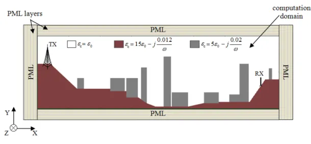
arrangement for the FDTD propagator developed by the authors in [8],[9] is used. Fig.1 illustrates a

typical 2D propagation scenario. In the same manner, it is adopted a vertical polarized signal modeled

(3)

general information of the propagation environment ((Earth curvature, inhomogeneous irregular

terrain, urban constructions, atmospheric refractive index, etc) are added to the mesh via electrical

parameters.

Fig. 1. Example of a two-dimensional environment configuration for the FDFD method.

The initial point of the FDFD formulation development is done as in [14] and [16]. It starts from the

Helmholtz equation instead of the traditional approach to use the separate one order derivative

Ampere's and Faraday's law. Although it becomes more complicated to obtain the final FDFD

expressions, this procedure minimizes the number of field components of the problem and

consequently the unknown variables of the linear system. In the present paper, different from the

previous mentioned works, it is applied the SCPML [18] structure in order to achieve higher wave

absorption and numerical performance [19].

Thus, assuming a time dependence of the form of

e

jt, where



is the angular frequency, the

Helmholtz equation is written for the magnetic field

H



:

) , ( ) , ( ) , ( ) , ( 1 0 2 y x M j y x H y x H y x s c

s      

 













(1)

and



_c

(

x

,

y

)

is the complex electric permittivity of the medium, which can assume complex values to

include losses in the form of







_c

(

x

,

y

)



(

x

,

y

)



j

(

x

,

y

)

(2)

where



is the electric conductivity of the medium.

M



(

x



,

y



)

is the magnetic current source,



₀ is

the magnetic permeability of the vacuum and the 2D operator



_s is given by

y y s x x

s_x _y

s ˆ 1 ˆ 1        ₍₃₎

The PML scale factors are







0

)

(

1 j

u

s

PML u u





y

x

(4)

where



₀ is the electric permittivity of the vacuum. In this way, the wave is attenuated inside the

PML region by the artificial conductivity



_uPML

(

u

)

to avoid reflections back to the computation

domain and therefore simulating infinite free space. The conductivity profile



_uPML

(

u

)

is defined

inside the PML only and is zero outside.

For vertical polarization, i.e., TEz mode, only the

H

_z field is enough to compute the problem

solution [20]. Hence, Eq. (1) is expanded in the scalar form of

)

'

,

'

(

)

,

(

)

(

)

(

)

,

(

)

(

)

,

(

1 )

(

)

,

(

)

(

)

,

(

1 )

(

0 2

y

x

M

j

y

x

H

y

s

x

s

y

x

H

y

s

y

x

y

x

s

x

y

x

H

x

s

y

x

y

s

z z y x z y c x z x c y











































(5)

Now, Eq. (5) is discretized by second order central finite-difference approximation and the

electromagnetic field components are distributed according with Yee's cell scheme [21]. The domain

is subdivided with spatial increment



x





y





and the indexes

i

and

j

indicate the number of

cells in the

x

ˆ

and

y

ˆ

directions respectively. So, after some extensive mathematical manipulations,

the final algorithm for the determination of

H

_z is

j i z j i c j i z j i z j i z j i z j i

z C H C H C H C H j M

H

C         5 ,  2 , ,

1 , 4 1 , 3 , 1 2 , 1

1



(6)

and the coefficients are given by:

 

1 2 3 4

2 2 , 5 2 / 1 4 2 / 1 3 2 / 1 2 2 / 1 1 C C C C s s k C s s C s s C s s C s s C j y i x j i j y i x j y i x j x j y j x j y               (7)

where

k

i,j is the complex wave number

k

i,j







₀



_ci,j . Here we adopt the work of Marengo et al.

[22] and choose the following PML conductivity profile for N-8 layers:

7 ,..., 2 , 1 , 0 16 2 02 . 0 8 ,..., 3 , 2 , 1 16 1 2 02 . 0 7 . 3 2 / 1 7 . 3                     i i i i PML i PML i



(8)

The problem solution is achieved by applying Eq. (6) at each grid point of the domain. Therefore,

the field values of all points must be found simultaneously. This leads to a system of linear equations

B

Ax



, where

A

is the coefficient matrix assembled according the propagation environment,

x

represents the unknown

H

_z values and

B

is a column vector specified by the current

M

_z .

The matrix

A

is highly sparse, has an unsymmetrical structure and for typical propagation

situations is very large. For such class of linear systems, iterative methods are preferred to direct

methods due the memory required. Besides, they often produce the solution faster than direct methods

(5)

At this point, we used routines from the Math Kernel Library (MKL©) provided by Intel© for Fortran

compilers [23].

III. RESULTS AND DISCUSSION

In this Section, three case studies are presented and preliminary results are generated. The

simulations were performed in a personal computer with a 3.4 GHz processor and 32 GBytes of

memory.

A. Method validation - canonical problem

First, it is investigated a canonical problem of an infinite magnetic line source placed at a height

h

above an infinite perfectly electric conductor (PEC) plane. The analytical solution can be obtained by

Image Theory, where the plane is replaced by a virtual source to account for the reflections from the

surface. The total field is the sum of the direct ray from the magnetic line and the field generated by

the virtual source (reflected ray from the ground), given in terms of Hankel functions [20].

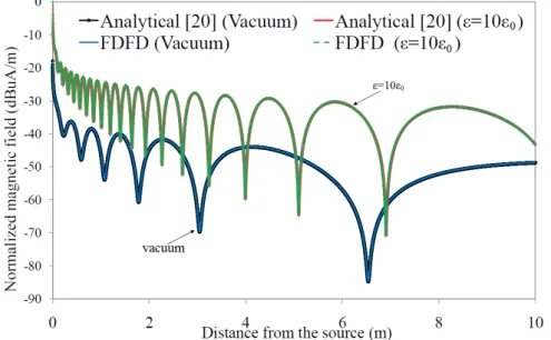
Two distinct situations are studied: the background medium above the infinite plane defined by

0





(vacuum) and





15 

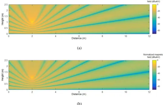
₀. The line source radiates a 1 GHz sinusoidal field located at 1 m

height. The FDFD is simulated with spatial discretization







/

40

. Fig. 2 exhibits the magnetic

field intensity for the vacuum case computed by the analytical formulation (a) and estimated by the

FDFD method (b).

(a)

(b)

Fig. 2 Magnetic field intensity distribution for the canonical problem of an infinite line source above a PEC plane. The background medium is vacuum. The results computed by the analytical solution [20] are exhibited in (a) and (b) presented

the data estimated by the FDFD method.

Fig. 3 shows the results for the magnetic field observed at points with

h



1

m and distance relative

to the source varying from 0.1 to 10 m. Here both the background medium situations are analyzed.

One can see a very good agreement between the analytical solution and the FDFD results. This

(6)

3 demonstrate the successful application of the PML in a non-homogeneous computation domain.

Fig. 3. Magnetic field for the problem of a PEC conductor illuminated by an infinite line source in different background mediums. Observation points with h = 1 m and distances varying from 0.1 to 10 m.

B. Cellular system measurements

The FDFD propagation analysis in a real urban environment is performed through a cellular system

measurement campaign carried out in Belo Horizonte, Brazil. The tests were performed during

November–December 2014, headed by the Brazilian National Telecommunication Agency

(ANATEL). The base station is placed at the Federal University of Minas Gerais (UFMG) in an

irregular terrain region, and the environment is mainly urban with several buildings and constructions.

The vertical polarized signal was generated at 2.16 GHz by a 46-dBm power transmitter, and the base

station antenna installed 50 m above the ground. Fig. 1 shows the environment configuration for a

link between the transmitter and a chosen measured point. The received power were recorded at 60

points distributed around the base station, whose distances from the source vary from 40 to 500 m.

The mobile unit used an omni-directional antenna at 1.8 m height. The campaign detailed information

can be found in [9] .

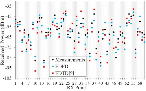
Fig. 4 exhibits the received power estimated via the proposed FDFD method, the results from the

FDTD propagator developed in [8], [9] and the measured data. In order to compare 2D propagation

methods directly to measurements or 3D formulations, the spherical wave attenuation with distance is

added likewise in [9] and [24]. So, the finite-difference fields are multiplied by a correction factor CF:





2

1 

CF

(9)

where



is the wave length and



is the distance between the source and the receiver.

In the present case, the FDTD is also implemented with second order central finite-difference

(7)

the following electric parameters:





15 

₀ and





0 .

0012

S/m for average terrain and





5 

₀

and





0 .

002

S/m for the urban buildings [25]. Moreover, the FDTD algorithm employed a moving

window of 20% of the respective TX-RX distance.

Fig. 4.Measured and estimated power at 60 observation points for the cellular system case. The receiver-transmitter distances vary from 40 to 500 m.

The prediction models accuracy can be analyzed in the scatter plot depicted in Fig. 5. For additional

comparison, the received power were also computed using an integral equation technique solved by

the Method of Moments (MoM) [6]. The diagonal reference line indicates a perfect agreement

between the estimated and the measured values. So, points above the reference line indicate a

predicted received power greater than the measurement. On the other hand, a point below the diagonal

line represents an underestimated received power. Moreover, Table I summarize the statistical

(8)

Brazilian Microwave and Optoelectronics Society-SBMO received 27 Apr 2018; for review 17 May 2018; accepted 09 Aug 2018 Fig. 5.Scatter plot for the cellular system case study.

TABLE I. ERROR STATISTICS FOR THE CELLULAR SYSTEM CASE STUDY.

Method Mean value error [dB]

RMS error [dB]

Standard deviation

[dB]

Total Simulation time [hour]

MoM [6] 6.1 11.1 9.4 9.3

FDTD [9] -3.4 7.4 6.9 763.5

FDFD 2.3 5.6 6.2 408.7

The signal coverage area of the base station is investigated in Fig. 6. The coverage map is obtained

performing the interpolation of the signal strength observed at the 60 measurement points. As the

points are not uniformly distributed, it cannot be delineated evenly spaced radials to scan the area and

produce a smooth continuous signal coverage figure as done in [26]. So, the distance between two

points varies different inside the region of interest.

The interpolation is computed by a Delaunay triangulation of the points and linear approximation

inside each triangle [27]. Due to the city constructions, it was not possible to acquire points to

compose a perfect circular area. Furthermore, the received power was recorded inside a 500-m radius

cell. Fig. 6.a presents the measured signal, whereas Fig. 6.b displays the predicted result via FDTD

method [9]. The coverage map estimated by the MoM technique [6] is depicted in Fig. 6.c and the

(9)

Brazilian Microwave and Optoelectronics Society-SBMO received 27 Apr 2018; for review 17 May 2018; accepted 09 Aug 2018 Fig. 6. Signal coverage area for the cellular system case study: (a) Measured signal, (b) predicted by the FDTD method [9],

(c) estimated by MoM technique [6] and (d) proposed FDFD results.

The results show a better performance of the FDFD method. The FDTD propagator also computed

values close to the measurements, but at much longer simulation times. Thus, an important difference

here is the computation cost. Nevertheless, as a time domain method, the FDTD can produce results

over a large frequency range on a single computer simulation.

The finite-difference methods incorporate the buildings heights in a straightforward manner via

mesh electrical parameters. Once the MoM method developed in [6] is restricted to smoothly

geometries, the results presented in this Section do not consider the buildings, only the irregular

ground. An important point here is the inclusion of the wave back-scattering, once the urban scenario

has a lot of obstacles. The FDFD technique has the potential to include all the radio wave propagation

mechanisms in the entire domain. The FDTD can consider the backward waves only inside the same

virtual window and the MoM method neglects the back-scattering.

C. Two-dimensional signal intensity distribution

In this section, we study the two-dimensional signal distribution or the coverage diagram in the

(10)

components, i.e., direct, diffracted, reflect and refracted contributions on the solution of the

propagation method. So, it is reproduced here an idealized example studied by Wang et al. [7], where

two rectangular buildings over flat terrain are illuminated by a 900 MHz signal. The structures are

assumed perfectly electric conductors and the transmitter antenna has a Gaussian pattern positioned at

38 m above the ground. In the mentioned work, the authors employed the two-way PE method solved

by Fourier split-step algorithm.

Fig. 7 presents the normalized received power obtained by the MoM [6] , FDTD [9] and FDFD

respectively. The results were generated with







/

10

. As expected, the back-scattering has great

influence on the final field composition and each method treats it in a different level, as discussed in

Section III.B. In this case, the FDTD employed 3 virtual windows. Although the MoM technique is

not developed for non-smoothly geometries, the comparison is still valuable. Regarding the

simulation time, the FDTD achieved the solution in 16 hours and the FDFD method in 1.7 hour.

However, the FDTD technique required 3.1 Gbytes of RAM while the FDFD 7.7 Gbytes.

(11)

Brazilian Microwave and Optoelectronics Society-SBMO received 27 Apr 2018; for review 17 May 2018; accepted 09 Aug 2018 (b)

(c)

Fig. 7.Two-dimensional signal intensity distribution in an idealized urban environment [7] estimated by (a) MoM technique[6], (b) FDTD method [9] and (c) proposed FDFD propagator.

IV. CONCLUSION

This paper presents a FDFD propagation method for complex urban environments. In addition of

the developed new formulation, the main novelty here is the application of the FDFD technique in

outdoor propagation problems. The method is validated through a canonical problem and then a

cellular measurement campaign are analyzed. Those results are compared to previous prediction

models implemented by the authors, namely a FDTD propagator and a MoM technique. The FDFD

achieved the smaller RMS error of 5.6 dB. Moreover, we exhibited a two-dimensional signal

distribution in an idealized urban scenario in order to visualize the effect of the wave components

(direct, diffracted, etc) on the solution. For both study cases, one can note the contribution of the

back-scattering in each method result. An important issue when dealing with the FDFD method is the

solution of the large and highly sparse linear systems. In this work it was adopted the iterative CGS

method, but there are others efficient schemes in literature and the authors intend to investigate it in

further works.

ACKNOWLEDGMENT

This work was partially supported by the Brazilian agencies CAPES, FAPEMIG and CNPq.

REFERENCES

[1] L. Sevgi, "Groundwave Modeling and simulation strategies and path loss prediction virtual tools", IEEE Transactions on Antennas and Propagation, vol. 55, No.6, pp.1591-1598, 2007.

[2] J. T. Hviid, J. B. Andersen, J. Toftgard, J. Bojer, "Terrain-based propagation model for rural area-an integral equation approach", IEEE Transactions on Antennas and Propagation, vol. 43, No. 1, pp.41-46, 1995.

[3] L. Sevgi, F. Akleman, "A novel finite-difference time-domain wave propagator", IEEE Trans. on Antennas and Propagation,vol. 48, No. 3, pp. 839-841, 2000.

[4] F. Agelet, A. Formella, J. Rabanos, F. Fontan, “Efficient Ray-tracing Acceleration Techniques for Radio Propagation Modeling”,

IEEE Transactions on Vehicular Technology, vol.49 , No.6 , pp.2089-2104, 2000.

(12)

[6] C. Batista and C. Rego, “An integral equation model for radiowave propagation over inhomogeneous smoothly irregular terrain”,

Microwave and Optical Tech. Letters, vol.54, pp.26-31, 2012.

[7] K. Wang, Y. Long, “Propagation modeling over irregular terrain by the improved two-way parabolic equation method”, IEEE Transactions on Antennas and Propagation, vol.60, No.9, pp.4467-4471, 2012.

[8] C. Batista and C. Rego, “A high-order unconditionally stable FDTD-based propagation method”, IEEE Antennas and Wireless Propagation Letters, vol.12, pp.809-812, 2013.

[9] C. Batista, C. Rego, M. Nunes and F. Neves, “Improved high-order FDTD parallel propagator for realistic urban scenarios and atmospheric conditions”, IEEE Antennas and Wireless Propagation Letters, vol.15, pp.1779-1782, 2016.

[10] F. T. Pachon-Garcia, "Modeling ground-wave propagation at mf band in hilly environments through fdtd method and interaction with gis", AEU - International Journal of Electronics and Communications, vol. 70, No. 8, pp. 981-989, 2016.

[11] G. Apaydin, C. Lu, L. Sevgi and W. Chew, “A Groundwave Propagation Model Using a Fast Far-Field Approximation”, IEEE Antennas and Wireless Propagation Letters, vol.16, pp.1369-1372, 2017.

[12] Y. Yang, Y. Long, "Modeling EM pulse propagation in the troposphere based on the TDPE method", IEEE Antennas and Wireless Propagation Letters, vol. 12, pp.190-193, 2013.

[13] W. Shin, 3D, Finite-difference frequency-domain method for plasmonics and nanophotonics, Ph. D. thesis, Stanford University, CA, USA, 2013.

[14] C. M. Rappaport, Q. dong, E. Bishop and M. Kilmer, “Finite difference frequency domain (FDFD) modeling of two dimensional TE wave propagation and scattering”, 2004 URSI International Symposium on Electromagnetic Theory, Pisa, Italy, May, 2004.

[15] Y. Zhao, K. Wu and K. Cheng, “A compact 2-D full-wave finite difference frequency-domain method for general guided wave structures”, IEEE Transactions on Microwave Theory and Techniques, vol.50, No.7, pp.1844-1848, 2002.

[16] O. M. Ramahi, V. Subramanian and B. Archambeault, “A simple finitedifference frequency-domain (FDFD) algorithm for analysis of switching noise in printed circuit boards and packages”, IEEE Transactions on Advanced Packaging, vol.26, No.2, pp.191-198, 2003. [17] V. Simoncini and D. Szyld, “Recent computational developments in Krylov subspace methods for linear systems”, Numerical Linear

Algebra with Applications, vol.14, No.1, pp.1-59, 2007.

[18] W. C. Chew and W. H. Weedon, “A 3-D perfectly matched medium from modified Maxwell’s equations with stretched coordinates”,

Microwave and Optical Tech. Letters, vol.7, No.13, pp.599-604, 1994.

[19] J.-P. Berenger, Perfectly Matched Layer (PML) for Computational Electromagnetics, Morgan & Claypool Publishers, 2007. [20] C. A. Balanis, Advanced Engineering Electromagnetics, 1ed, John Wiley and Sons Wiley, 1989.

[21] K. S. Yee, “Numerical solution of initial boundary value problems involving maxwell’s equation in isotropic media”, IEEE Trans. onAntennas and Propag. , vol. ap.14, No. 3, pp.302-307, 1966.

[22] E. A. Marengo, C . M. Rappaport and E. L. Miller, “Optimum PML ABC Conductivity Profile in FDFD”, IEEE Trans. on Magnetics,

vol.35, No.3, pp.1506-1509, 1999.

[23] O. Schenk and K. Grtner, “Solving unsymmetric sparse systems of linear equations with PARDISO”, Future Generation Computer Systems, vol.20, No.3, pp.475-487, 2004.

[24] Y. Wu, M. Lin and I. Wassell,, “Path loss estimation in 3D environments using a modified 2D Finite-Difference Time-Domain technique”, IEEE 7th International Conference on Computation in Electromagnetics (CEM 2008), Brighton, UK, pp.98-99, 2008. [25] H. L. Bertoni, Radio Propagation for Modern Wireless Systems. Englewood Cliffs, NJ, USA, Prentice-Hall, 2000.

[26] C. Batista, C. Rego, M. Evangelista, G. Ramos, Application of analytical propagation models on point-to-point and point-to-area RF signal prediction, 9th European Conf. on Ant. and Propag. (EUCAP 2015), Lisbon, Portugal, April, 2015.