Abstract— The definition of parameters that characterize the radiation of electric and magnetic fields for antennas in the time and frequency domain on an unified representation is proposed. The formulation uses a straightforward semi-analytical formulation that can be subsequently applied on the analysis of excited antennas for an arbitrary source with temporal behavior. The effective height is a parameter for antenna analysis defined for quantities in far field region and can be used as a transfer function of the antenna. This transfer function can be described through the antenna singularities which can be obtained by singularity expansion. The Singularity Expansion Method (SEM) is capable to model an electromagnetic quantity with the singularities extracted by the current densities of an arbitrary object. This work proposes that the singularities are extracted by the Matrix Pencil method applied on the current densities. The current densities are obtained numerically through the method of the Finite Differences in the Time Domain (FDTD) for wired log-periodic antenna and, after the singularities are obtained, the formulation of the semi-analytical effective height equation is written. To validate the presented method, a formulation of the time-domain radiation pattern is presented and a corresponding frequency-domain radiation pattern is also presented using Parseval’s theorem.
Index Terms— SEM, FDTD, Effective Height, Matrix Pencil.
I. INTRODUCTION
In most cases, electromagnetism problems analysis methods presume the electric and magnetic
fields and their associated quantities have harmonic temporal behavior. This indicates that the
solutions are found in frequency domain since in this domain the computation of the solutions is
straightforward. The corresponding temporal solution is obtained through the inverse Fourier
transform.
Semi-analytical formulation for a Unified
Time and Frequency Antenna Characterization
S. T. M Gonçalves
Department of Electrical Engineering, Federal Center of Technological Education of Minas Gerais
C. G. do Rego
However, harmonic electromagnetic fields have been used for decades in project and analysis of
mathematics models and devices like sources and antennas for wireless communications. Antennas
and excitation sources design have been developed in frequency domain to obtain lower cost and
higher efficiency. Therefore, frequency domain methods are more appropriated to analyze
narrowband antennas.
If a wideband antenna is required, a frequency domain method has considerable difficulties since
the solution must be found in each frequency with significant magnitude of the problem. If a huge
amount of frequencies is present in the analyzed fields, frequency domain methods may be not the
best choice to find the radiated fields by this wideband antenna.
Many electromagnetic problems can be solved directly in time domain. However, greater memory
and computer processing is required in these cases. The hardware enhancement of personal computers
has enabled time domain methods to solve some electromagnetic problems with less mathematical
calculations. In these cases, the solution is obtained faster that in frequency domain methods [1].
The numerical analysis in temporal domain has motivated the study of wideband signals. Good
results were obtained and validated by experimental measure [2]. More recently, a large effort has
been made to apply temporal domain methods to wideband antennas and fields calculations.
Parameters are defined directly in time domain which increase insight about how the energy radiates
when considering the complete signal with all its frequencies instead of frequency to frequency
analysis [3], [4].
The most widely method used to numerically solve electromagnetic equations in time domain is the
Finite Difference in Time Domain (FDTD) method, proposed by Yee in 1966 [5]. However, the
FDTD is a numeric method and does not provide an analytical solution which characterizes an
antenna and its radiated energy.
An analytical solution can be obtained even for a complex geometry antenna or non-harmonic
excitation source using the effective height [4]. The effective height is, in essence, a transfer function
of an antenna and describes the relationship between the input voltage signal and the radiated field. It
can be described in time and frequency domain.
It is possible to describe the effective height through an unified way which is capable to easily be
exchanged between frequency and time domain formulations. The Singularity Expansion Method
(SEM) [6] is proposed to define the effective height since the SEM is a representation of a quantity as
time and frequency domain which is the reason the effective height becomes unified between time and
frequency domains.
The SEM raised from the necessity of analyzes scattering fields of objects and signals radiated by
narrow pulse fed antennas. However, the SEM can be used to develop any wideband model, not just
the pulsed ones.
The singularity extraction from experimental data was implemented by [2]. Recently works have
been applied SEM through current density and radiated fields [7]. However such approach has
disadvantages. If the excitation is changed, all singularities must be recalculated. The effective height
is a transfer function so the excitation can be changed arbitrarily.
In this work the SEM is used to obtain a unified effective height in time and frequency domains.
The singularities can be extracted from the analytical response but this limits the analysis to simple
geometries. Thus, the singularities are extracted directly by a temporal numerical method using fields
and current densities that is obtained by FDTD. The Matrix Pencil method was chosen to extract the
singularities from the temporal electric and magnetic current densities because it is very efficient and
robust [8]. Since the singularities are obtained numerically, the formulation of the effective height is
so called semi-analytical. Concomitantly with the development of this work, the use of SEM and
effective height was implemented in [9] where a surface is defined around the antenna instead using
the antenna surface itself and the singularities are extracted from the currents and fields of this
spherical surface.
An impulsional response of an antenna is needed for the singularity extraction. As known,
analytical response from impulsional source can be obtained for simple antennas. However, in more
complex cases an analytical response cannot be found. Therefore, the semi-analytical approach can be
useful to obtain wideband time and frequency domain response. A Log-Periodic Dipole Array
(LPDA) is a wired antenna that is wideband and has not an analytical formulation which describes the
energy scattering. Thus, this antenna was chosen to elucidate the approach. In order to validate the
results, the same geometry was simulated by Method of Moments (MoM) which can handle very well
wired antennas and produces results with high precision. A comparison between MoM and
semi-analytical effective height can be done by Fourier transform of the time-domain results. However, to
easy the process a simple and faster approach is used. The radiation pattern of the LPDA is defined by
the energy of the signal normalized by its maximum. Using the Parseval’s theorem it can be proved
This work is organized as follows. The singularity expansion method for modeling the transient
radiation phenomena is analyzed in Section II. The Matrix Pencil method and the selection of
contributing singularities are presented in Section III. Section IV describes the effective height of an
antenna and Section V presents the LPDA modeling. Parserval’s theorem used to define time and
frequency domains radiation pattern is presented in Section VI. The application of the proposed
methodology to the analysis of the LPDA is then presented in Section VII. The concluding remarks
are summarized in Section VIII.
II. SINGULARITY EXPANSION METHOD
As known, the scattered field from any object by an incident pulse wave has two components: the
Early-Time which represents the direct reflection of the incident pulse and the Late-Time which
represents the resonance of the natural frequencies and causes a damped-oscillatory behavior at the
scattered field. The natural frequencies are associated with the geometry and electrical properties of
the scatter. The Early Time is often too short and can be disregarded (except in a very electrically
large structure) [10].
After the incident pulse wave is dead, some response still can be measured. This occurs due the
oscillation at the natural frequencies of the object. A scattered field by these natural frequencies can
be decomposed in a sum of exponentially damped sinusoids which in frequency domain represents a
pair of poles and residues. A singularity is defined as a pair of pole and its corresponding residue. The
procedure of finding all singularities and building an electric or magnetic response with them, is
called Singularity Expansion Method.
The scattering response of an arbitrary object can be written as [10]
, = −, + , , , (1)
where , is the quantity modeled by SEM ( represents the quantity which the singularities
are extracted). The sum adds the contribution of each singularity extracted from the object. The
− term represents the contribution of the poles where indicate the pole order. The term
, is the coupling coefficient multiplied by the natural mode. This term can be analyzed through the object geometry and its electrical characteristics but with numerical extraction of
singularities, such analysis is not necessary because this term is directly determined [11]. The
III. MATRIX PENCIL AND SELECTION OF CONTRIBUTING OF NATURAL POLES
There are two methods widely used to extract singularities from a temporal response: Prony and
Matrix Pencil. However, the Matrix Pencil method is more efficient and robust [2].
Each natural frequency obtained by the Matrix Pencil method contributes to some degree or another
to build the response. Some of them can be disregarded because they have not sufficient energy to
affect the scattered fields. Eliminating these natural frequencies, decrements the overall time
simulation.
The significant natural frequencies can be obtained by a pre-defined criterion [12]. Among the
extracted singularities, there will be a smaller singularities number which corresponds to the natural
frequencies. The Matrix Pencil provides the singularities in the form of a pair of poles and residues.
These poles and residues can be used to define an energy criterion for selection of the contributing
singularities extracted by the Matrix Pencil. Using a threshold ℎ, an expression can be written
according with [12],
< ℎ, (2)
where = |! | |" |⁄ is a weight defined to account the effect of this singularity and is the higher
amplitude which is used to normalize the weights. Singularities that satisfy the Equation (2) are
eliminated.
However, the Equation (2) is not sufficient for all cases. In some objects there are singularities that
do not contribute to the overall response but are not eliminated by the Equation (2) criterion. These
singularities are responsible for fast response, occur before the Late Time and must be eliminated. The
elimination of these singularities can be made by the following criterion [12].
|" | > |"%&'|, (3)
where ()|*+,-|./ ≈ ℎ and 1 is the beginning of the Late Time.
IV. EFFECTIVE HEIGHT AND THE SEMI-ANALYTICAL FORMULATION
The effective height can be defined as the relationship between the excitation voltage and the
23 4, 5 = 6
65 7 89:;< , = +4 ⋅? @ + 1 B;< , = +4 ⋅? @ C 4D dF
GH . (4)
The electric field is written using the formulation of the effective height expressed in Equation (4),
J , 5 = −4MN O2K 3 4, = ∗ Q = R, = = 5 −N
?, (5)
where the 5 index in Equation (4) indicates a transmitter antenna. The current densities in time domain
originated by a pulsed excitation is represented by 9; and B; and the argument = +4⋅TH is the delay
from the excitation point to observer where and are observer and source coordinate system. In
Equations (4) and (5) ? is the speed light, is the intrinsic impedance of vacuum and K is the
permeability of vacuum. The function Q = is an arbitrary excitation.
With the SEM formulation, the impulsional current densities can be described in function of the
object singularities which are extracted by the Matrix Pencil. In this work, the object is built with
perfect electric conductor so there are just single order poles [6].
9; , = U 9 ,
− , (6)
B; , = U B ,
− , (7)
where U , = , V is the residue obtained by the Matrix Pencil [11]. Thus, in terms
of the object singularities, the effective height can be written as
23 4, 5 = W X5 −N
?Y U2
Z
, ([ X3)\TY (8)
and
U2Z , = 7 OU9: , + 1 UB , C 4R
GH (
[ ]4⋅T ^H
dF . (9)
Through the Laplace transform, the corresponding frequency domain ( = _`) can be obtained in a
23 4, 5 = ()[\T U2
Z ,
− , (10)
U2Z , = 7 OU 9: , + 1 U B , C 4R
GH (
[]4⋅T ^H dF . (11)
The Equations (8) - (11) define in a unified way the effective height since it is simple to transform
to and from time or frequency domain. It is a tool for far field analysis with a semi-analytical formula.
V. LOG-PERIODIC DIPOLE ARRAY
LPDA antennas are known as frequency independent and can used in wideband applications.
Although using MoM provides good results when applied on wired antennas, an analytical solution is
very hard to obtain to this antenna when excited by wideband signals. Even MoM can have a highly
computational cost for wideband signals. To illustrate the use of the purposed semi-analytical
effective height, the results in frequency domain are compared with MoM results. Table I and Fig. 1
describes the LPDA used in this work. The bandwidth of this antenna is from 18.064 de to
44.102 de, obtained by the resonance of the bigger and smaller dipoles [11]. It can be seen that this LPDA has a significant size.
TABLE I. LPDA SIZES
Segment Length (g) Radius (gg) Segment Length (g) Radius (gg)
1 4.1518 15.875 12 0.1524 0.5131
2 4.1518 15.875 13 0.9964 0.5131
3 3.3214 12.7 14 0.7974 0.5131
4 3.3214 12.7 15 0.6376 0.5131
5 2.6572 9.525 16 0.5102 0.5131
6 2.6572 9.525 17 0.1524 0.5131
7 2.1257 7.9375 18 0.9964 0.5131
8 2.1257 7.9375 19 0.7974 0.5131
9 1.7006 6.35 20 0.6376 0.5131
10 1.7006 6.35 21 0.5102 0.5131
Fig. 1. Elements numbers of the LPDA fed by the front end.
Through FDTD, the LPDA can be simulated using the following parameters: the cell size can be
found analyzing the resonance frequency of one of the several half-wave dipoles. The relationship
between the maximum frequency in the computational domain and the segmentation of the antenna
can be expressed as [11]
l[mn=ℎQ%&'? lo, (12)
where l[mn is the number of segments, ℎ is the size of the chosen dipole, ? is the speed of light, Q%&'
is the maximum frequency with significant amplitude present in the computational space and lo is the
mesh resolution, usually set for 10 or 20 [13], is defined as the ratio between the p%q = ?/Q%&' and
the FDTD cell size Δ. In order to determine Q%&', we choose the value of twice the resonance of a
half-wave dipole as considered in [11]. The resonance of the half-wave dipoles of the LPDA in Fig. 1
is greater for the small dipole consisting of the elements 9 and 10. Thus, since Q = ?/p is the
resonance frequency, ℎ = p /2 so Q = ?/2ℎ. Finally, Q%&' = 2Q. With these parameters set and
lo = 20 to lesser dispersion level, the number of segments of elements 9 and 10 is l[mn = 20. The cell size can be determined as
Δ =
ℎ
[mn:u & vl
[mn
,
(13)and the others segments can be defined as
where l is the number of cells of an element defined by a length ℎ[mn: .
The final modeling of the FDTD space is determining the time step size for a tridimensional grid.
Since Δ5 = Δ/√3, the times step is Δ5 = 3.275 C 10)v .
The excitation of the LPDA must excite all natural frequencies so an approximate impulsional
current density can be determined. However, the LPDA has a bandwidth limited by high and low
frequencies which are function of the resonance frequency of front-end and back-end dipoles. A
Gaussian pulse is a natural choice and widely used to extract natural frequencies since it has a
well-known behavior. Nevertheless, a Gaussian pulse has large amount of low frequencies. This can be
avoided using the first derivative of the Gaussian pulse because this waveform does not contain low
frequencies and DC component as seen in Fig. 2 and Fig. 3.
Fig. 2. First derivative of the Gaussian pulse for {| = }. ~•€ C •‚)•‚ ƒ.
It is important that the excitation does not contain frequencies out of the band of the antenna
because very low frequencies cause errors on the singularities extraction by the Matrix Pencil and
very high frequencies cause dispersion error in the FDTD grid.
The SEM formulation for the LPDA is presented as follows. Considering that the singularities were
extracted by Matrix Pencil method, the semi-analytical formulation as described in Equation (9) can
be determined as
!…2„Z† , = 7
GH ! „
9 , ([ ]'H‡ˆ‰ „ Š‹‡ Œ•ŽH‡ˆ‰ „ ‡ˆ‰ Œ••T HŠ‹‡ „^dF (15)
and
!…2ŒZ† , = 7
GH ! Œ
9 , ([ ]'H‡ˆ‰ „ Š‹‡ Œ•ŽH‡ˆ‰ „ ‡ˆ‰ Œ••T HŠ‹‡ „^
dF , (16)
where there are not ! B , terms because the LPDA has only perfectly electric conductors.
Finally the effective height can be determined by Equation (8).
VI. PARSEVAL’S THEOREM
The Parseval’s theorem implies that the energy of a temporal signal • 5 ∈ ℝ has the same
magnitude of the frequency spectrum energy, obtained by the Fourier transform “ ` of the temporal
signal • 5 . This can be expressed as
7 |• 5 |”•5 = 7 |“ ` |– ”•` )–
–
)– . (17)
The radiation pattern in the frequency domain is calculated using the square of quantity module like
the electric far field or the radiation intensity. Thus, using the Parseval’s theorem, if a sinusoidal
waveform is used as excitation Q = in Equation (5), the temporal response obtained by the effective
height can be validated - using another frequency domain method, like MoM - without any Fourier
transform of the temporal effective height response. To accomplish that, the radiation pattern must be
defined as the signal energy normalized by its maximum since the energy is the same in time and
frequency domain.
To summarize the whole process of obtain and validate the semi-analytical effective height, a
Fig. 4. Fluxogram of the effective height determination and validation
VII. RESULTS AND DISCUSSION
With the LPDA defined, the results obtained by the semi-analytic effective height are compared
with the same LPDA simulated by MoM through the software 4l—˜2 [14]. Since the bandwidth of
this antenna is from 18.064 de to 44.102 de, to illustrate and validate the effective height, two
frequencies were chosen inside the LPDA bandwidth: 28.05 de and 34.05 de. The frequencies
near the limits of the band were avoided because the singularities are not well extracted on these
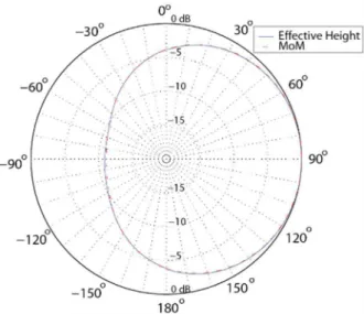
limits [11]. The Fig. 5-7 shows the radiation pattern obtained by MoM and effective height for the
™ = 0° and › = 90° planes.
Fig. 5. Radiation pattern obtained by effective height and MoM for the plane œ = ‚° at ~•. ‚€ žŸ . Effective height determined for LPDA
Time-domain radiation pattern Validation by MoM - using Parseval Matrix Pencil applied in current densities
Singularities extracted Selection of contribuiting singularities LPDA modeled in FDTD
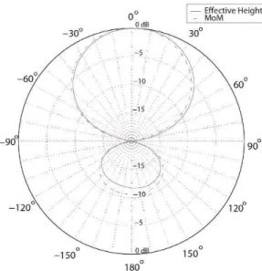
Fig. 6. Radiation pattern obtained by effective height and MoM for the plane ¡ = ¢‚° at 28.‚€ žŸ .
Fig. 7. Radiation pattern obtained by effective height and MoM for the plane œ = ‚° at 34.‚€ žŸ .
The slight differenced showed in Fig. 5-8 can be explained by the followings assumptions: FDTD
dispersion is significant on higher frequencies; Mur absorbing boundary condition was used;
modeling approximations; excitation frequency response has not uniform amplitude for all
frequencies; steady-state response of the LPDA currents take very long time to simulate, so the
currents are truncated in time. These factors does not affect the time and frequency response
significantly, however, they can degrade the singularities extraction. When singularities are shifted at
the complex plane, the effective height is slightly, but noticeable, affected. For instance, it can be
noted an asymmetry in the effective height in Fig. 6 and Fig. 8 which occur due the asymmetry
between a pair of complex poles that should not exist if analytical singularities determination were
carried out.
VIII. CONCLUSION
A semi-analytic effective height formulated with the Singularity Expansion Method was proposed.
The singularities were obtained numerically by the Matrix Pencil method applied on temporal currents
provided by FDTD. The semi-analytic effective height can be easily represented in time and
frequency domains and is very useful to obtain far-fields quantities in arbitrary positions and antenna
parameters like radiation pattern. The formulation was tested and validated comparing the radiation
pattern of a Log-Periodic Dipole Array antenna which has not analytical solution, with the Method of
Moments solution. The obtained results have good agreement but the simulation environment has to
be investigated and refined.
ACKNOWLEDGEMENT
This work was partially supported by CNPq, CAPES and FAPEMIG.
REFERENCES
[1] K. S. Kunz and R. J. Luebbers, The Finite Difference Time Domain Method for
Electromagnetics. CRC Press, Boca Raton, 1993.
[2] S. Licul, “Ultra-wideband antenna characterization and measurements,” Ph.D. dissertation,
Faculty of the Virginia Polytechnic Institute & State University, 2004.
[3] S. T. M. Gonçalves, “Caracterização temporal de antenas refletoras para faixas de frequência
ultra-largas,” Master’s thesis, Universidade Federal de Minas Gerais, 2005.
[4] A. Shlivinski, E. Heyman, and R. Kastner, “Antenna characterization in the time domain,”
[5] K. S. Yee, “Numerical solution of initial boundary value problems involving maxwell’s
equations in isotropic media,” IEEE Transaction on Antennas and Propagation, vol. AP–14, no. 3,
pp. 302–307, 1966.
[6] C. E. Baum, “The singularity expansion method,” Transient Electromagnetics Fields, 1976,
L. B. Felsen (editor), Berlin: Springer-Verlag.
[7] G. Marrocco and M. Ciattaglia, “Ultrawide-band modeling of transient radiation from
aperture antennas,” IEEE Transactions on Antennas and Propagation, vol. 52, no. 9, pp. 2341–2347,
Sep. 2004.
[8] R. S. Adve, T. K. Sarkar, O. M. C. Pereira-Filho, and S. M. Rao, “Extrapolation of
time-domain responses from three-dimensional conducting objects utilizing the matrix pencil technique,”
IEEE Transactions on Antennas and Propagation, vol. 45, no. 1, pp. 147–156, Jan. 1997.
[9] D. Caratelli and A. Yarovoy, “Unified time- and frequency-domain approach for accurate
modeling of electromagnetic radiation processes in ultrawideband antennas,” IEEE Transactions on
Antennas and Propagation, vol. 58, no. 10, pp. 3239–3255, Oct. 2010.
[10] C. E. Baum, “Singularity expansion of electromagnetic fields and potentials radiated from
antennas or scattered from objects in free space,” May 1973, Sensor and simulation notes, Air Force
Weapons Laboratory.
[11] S. T. M. Gonçalves, “Caracterização unificada de antenas nos domínios do tempo e
frequência”, Ph.D. dissertation, Universidade Federal de Minas Gerais, Sep. 2010.
[12] J. Chauveau, N. de Beaucoudrey, and J. Saillard, “Selection of contribuiting natural poles for
the characterizationa of perfectly conducting targets in resonance region,” IEEE Transactions on
Antennas and Propagation, vol. 55, no. 9, pp. 2610–2617, Sep. 2007.
[13] A. Taflove and S. C. Hagness, Computational Electrodynamics: The Finite Difference Time
Domain Method, 2nd ed. Artech House, Boston, 2000.
[14] A. Voors, “Nec based antenna modeler and optimizer,” http://www.qsl.net/4nec2/, last access