Escola de Engenharia Departamento de Inform´atica
Daniel Ara´ujo
Real-Time Intelligence
Escola de Engenharia Departamento de Inform´atica
Daniel Ara´ujo
Real-Time Intelligence
Master dissertation
Master Degree in Computer Science Dissertation supervised by
Paulo Novais - Universidade do Minho Andr´e Ribeiro - Performetric
Firstly and foremost, I would like to express my gratitude to my parents and my brother, for their support, they have always helped me to think more clearly, and without them this work would not have been possible.
I would also like to thank to my friends at Performetric, particularly to Andr´e Pimenta (co-supervisor), who was available at all times to provide technical guidance and friendship.
Last but not least, I would like to thank to Professor Paulo Novais for the supervision of this work and the motivation he provided.
Over the past 20 years, data has increased in a large scale in various fields. This explosive increase of global data led to the coin of the term Big Data. Big data is mainly used to des-cribe enormous datasets that typically includes masses of unstructured data that may need real-time analysis. This paradigm brings important challenges on tasks like data acquisi-tion, storage and analysis. The ability to perform these tasks efficiently got the attention of researchers as it brings a lot of oportunities for creating new value. Another topic with growing importance is the usage of biometrics, that have been used in a wide set of appli-cation areas as, for example, healthcare and security. In this work it is intended to handle the data pipeline of data generated by a large scale biometrics application providing basis for real-time analytics and behavioural classification. The challenges regarding analytical queries (with real-time requirements, due to the need of monitoring the metrics/behavior) and classifiers’ training are particularly addressed.
Key Words: Real-Time Analytics, Big Data, NoSQL Databases, Machine Learning, Bio-metrics, Mouse Dynamics
Nos os ´ultimos 20 anos, a quantidade de dados armazenados e pass´ıveis de serem proces-sados, tem vindo a aumentar em ´areas bastante diversas. Este aumento explosivo, aliado `as potencialidades que surgem como consequˆencia do mesmo, levou ao aparecimento do termo Big Data. Big Data abrange essencialmente grandes volumes de dados, possivelmente com pouca estrutura e com necessidade de processamento em tempo real. As especificida-des apresentadas levaram ao apareciemento de especificida-desafios nas diversas tarefas do pipeline t´ıpico de processamento de dados como, por exemplo, a aquisic¸˜ao, armazenamento e a an´alise. A capacidade de realizar estas tarefas de uma forma eficiente tem sido alvo de es-tudo tanto pela ind ´ustria como pela comunidade acad´emica, abrindo portas para a criac¸˜ao de valor. Uma outra ´area onde a evoluc¸˜ao tem sido not´oria ´e a utilizac¸˜ao de biom´eticas com-portamentais que tem vindo a ser cada vez mais acentuada em diferentes cen´arios como, por exemplo, na ´area dos cuidados de sa ´ude ou na seguranc¸a. Neste trabalho um dos ob-jetivos passa pela gest˜ao do pipeline de processamento de dados de uma aplicac¸˜ao de larga escala, na ´area das biom´etricas comportamentais, de forma a possibilitar a obtenc¸˜ao de m´etricas em tempo real sobre os dados (viabilizando a sua monitorizac¸˜ao) e a classificac¸˜ao autom´atica de registos sobre fadiga na interac¸˜ao homem-m´aquina (em larga escala).
Palavras-chave: Indicadores em tempo real, Big Data, Bases de dados NoSQL, Machine Learning, Biom´etricas Comportamentais
1 introduction 2 1.1 Motivation 2 1.1.1 Big Data 2 1.1.2 Real-Time Analytics 3 1.2 Context 4 1.3 Objectives 4 1.4 Methodology 5 1.5 Work Plan 5 1.6 Document Structure 5
2 state of the art 8
2.1 Data Generation and Data Acquisition 8
2.1.1 Data Collection 10
2.1.2 Data Pre-processing 11
2.2 Data Storage 11
2.2.1 Cloud Computing 12
2.2.2 Distributed File Systems 12
2.2.3 CAP Theorem 13
2.2.4 NoSQL - Not only SQL 14
2.3 Data Analytics 20
2.3.1 MapReduce 21
2.3.2 Real Time Analytics 23
2.3.3 MongoDB Aggregation Framework 24
2.4 Machine Learning 25
2.4.1 Introduction to Learning 25
2.4.2 Deep Neural Network Architecutres 28
2.4.3 Popular Frameworks and Libraries 30
2.5 Related Projects 31
2.5.1 Financial Services - MetLife 31
2.5.2 Government - The City of Chicago 31
2.5.3 High Tech - Expedia 32
2.5.4 Retail - Otto 32
2.6 Summary 32
3 the problem and its challenges 34
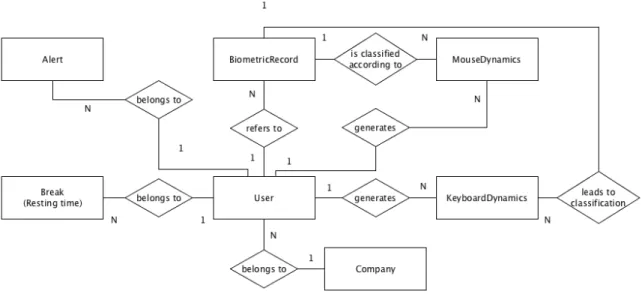
3.1.1 Data Model 36
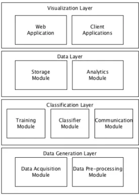
3.1.2 System Components 38
3.1.3 Deployment View 39
3.2 Rate of Data Generation and Growth Projection 40
3.2.1 Data Analytics 41
3.2.2 Data Insertion 42
3.2.3 Classifier Training 43
3.3 Summary 44
4 case studies 45
4.1 Experimental setup and Enhancements Discussion 45
4.1.1 MongoDB Aggregation Framework 45
4.1.2 Caching the queries’ results with EhCache 50
4.1.3 H2O Package 51 4.2 Testing Setup 53 4.2.1 Physical Setup 53 4.2.2 Data Collection 54 4.3 Results 57 4.3.1 Data Aggregation 58 4.3.2 Data Classification 63 4.4 Summary 65
5 result analysis and discussion 66
5.1 Data Aggregation 66
5.1.1 Simple queries results analysis 66
5.1.2 Complex queries results analysis 67
5.1.3 Caching queries results analysis 67
5.2 Data Classification 68
5.3 Project Execution Overview 69
6 conclusion 70
6.1 Work Synthesis 70
6.2 Prospect for future work 71
a queries response times 78
a.1 Company Queries Execution Performance 78
a.2 Team Queries Execution Performance 79
a.3 User Queries Execution Performance 81
a.4 Group By Queries Execution Performance 82
a.5 Hourly Queries Execution Performance 84
Figure 1 Work plan showing the timeline of the set of tasks in this
disserta-tion. 6
Figure 2 The Big Data analysis Pipeline according toBertino et al.(2011). 9 Figure 3 HDFS Architecture from https://hadoop.apache.org/docs/r1.2.
1/hdfs_design.html. 13
Figure 4 Mapping between Big Data 3 V’s and NoSQL System features. 14 Figure 5 Classification of popular DBMSs according to the CAP theorem. 15
Figure 6 Hadoop MapReduce architecture. 22
Figure 7 Pseudocode representing a words counting implementation in
map-reduce. 22
Figure 8 MongoDB Aggregation Pipeline example. 25
Figure 9 Bias and variance in dart-throwing (Domingos(2012)). 28 Figure 10 Functional model of an artificial neural network (Rojas(2013)). 29 Figure 11 Overview of the concepts presented in chapter 2. 33 Figure 12 Conceptual Diagram of the Data Model (according toChen(1976)). 37 Figure 13 The deplyment view (showing the layered architecture). 38 Figure 14 The deployment view (showing the devices that take part in the
sys-tem). 40
Figure 15 A representation of a sharded deployment in MongoDB. 43 Figure 16 Example of an aggregation pipeline (includes 2 stages). 47 Figure 17 Example of an aggregation pipeline (includes 3 stages). 48 Figure 18 Pseudocode representing the implementation of a simple MongoDB
query. 48
Figure 19 Pseudocode representing the implementation of a MongoDB
aggre-gation framework query. 49
Figure 20 Pseudocode representing the implementation of the case operator. 50 Figure 21 Example of usage of the defined cache (Java code). 51 Figure 22 Example of usage of neural networks with H2O (R code). 52
Figure 23 MongoDB replica set topology. 53
Figure 24 MongoDB replica set topology (after primary member becomes
un-available). 54
Figure 25 Example of JMH usage (Java code). 55
Figure 27 Piece of AWK code used for parsing the output generated by JMH. 57 Figure 28 Comparison between Java and MongoDB aggregation framework
implementations (queries about a specific company name) for a cur-rent time interval (see subsection 3.2.1). 59 Figure 29 Comparison between Java and MongoDB aggregation framework implementations (queries about a specific company name) for a past
time interval (see subsection 3.2.1). 59
Figure 30 Comparison between Java and MongoDB aggregation framework implementations (queries about a specific team name) for a current
time interval (see subsection 3.2.1). 60
Figure 31 Comparison between Java and MongoDB aggregation framework implementations (queries about a specific team name) for a past time
interval (see subsection 3.2.1). 60
Figure 32 Comparison between Java and MongoDB aggregation framework implementations (queries about a specific user name) for a current
time interval (see subsection 3.2.1). 61
Figure 33 Comparison between Java and MongoDB aggregation framework implementations (queries about a specific user name) for a past time
interval (see subsection 3.2.1). 61
Figure 34 Comparison between Java and MongoDB aggregation framework implementations (queries about a specific company name). 62 Figure 35 Comparison between Java and MongoDB aggregation framework implementations (queries about a specific team name). 62 Figure 36 Comparison between Java and MongoDB aggregation framework implementations (queries about a specific user name). 63 Figure 37 Comparison between previous and MongoDB aggregation frame-work implementations (query about data generated in the current
hour). 85
Figure 38 Comparison between previous and MongoDB aggregation frame-work implementations (query about data generated in the last hour). 86
Table 1 NoSQL DBMS comparison. 19
Table 2 Data growth projections. 40
Table 3 Data growth projections. 42
Table 4 Classifier training results. 64
Table 5 Throughput of a set of queries where data is filtered by company
name (Java implementation). 78
Table 6 Throughput of a set of queries where data is filtered by company
name (MongoDB Agg. implementation). 78
Table 7 Average time of a set of queries where data is filtered by company
name (Java implementation). 79
Table 8 Average time of a set of queries where data is filtered by company
name (MongoDB Agg. implementation). 79
Table 9 Throughput of a set of queries where data is filtered by group name
(Java implementation). 79
Table 10 Throughput of a set of queries where data is filtered by group name
(MongoDB Agg. implementation). 80
Table 11 Average of a set of queries where data is filtered by group name (Java
implementation). 80
Table 12 Average of a set of queries where data is filtered by group name
(MongoDB Agg. implementation). 80
Table 13 Throughput of a set of queries where data is filtered by user name
(Java implementation). 81
Table 14 Throughput of a set of queries where data is filtered by company
name (MongoDB Agg. implementation). 81
Table 15 Average time of a set of queries where data is filtered by company
name (Java implementation). 81
Table 16 Average time of a set of queries where data is filtered by company
name (MongoDB Agg. implementation). 82
Table 17 Throughput of a set of queries where data is grouped by time inter-vals according to labels (Java implementation). 82 Table 18 Throughput of a set of queries where data is grouped by time inter-vals according to labels (MongoDB Agg. implementation). 83
Table 19 Average times of a set of queries where data is grouped by time intervals according to labels (Java implementation). 83 Table 20 Average times of a set of queries where data is grouped by time intervals according to labels (MongoDB Agg. implementation). 84 Table 21 Throughput of a set of queries where the retrived data is from last 2
hours (Java implementation). 84
Table 22 Throughput of a set of queries where the retrived data is from last 2
hours (MongoDB Agg. implementation). 84
Table 23 Average time of a set of queries where the retrived data is from last
2 hours (Java implementation). 85
Table 24 Average time of a set of queries where the retrived data is from last
2 hours (MongoDB Agg. implementation). 85
Table 25 Throughput of the set of queries using the Cache system. 87 Table 26 Average time of the set of queries using the Cache system. 88
ACID Atomicity, Consistency, Isolation, Durability ANN Artificial Neural Network
API Application Programming Interface
BASE Basically available, Soft state, Eventual consistency BSON Binary JSON
CAP Consistency, Availability, Partition tolerance CRUD Create, Read, Update, Delete
DBMS Data Base Management System DFS Distributed File System
ETA Estimated Time of Arrival ETL Extract, Transform, Load GLM Generalized Linear Mode GPS Global Positioning System HTTP Hypertext Transfer Protocol IaaS Infrastructure as a Service JDK Java SE Development Kit JMH Java Microbenchmark Harness JSON JavaScript Object Notation JVM Java Virtual Machine KNN K-Nearest Neighbors MSE Mean Squared Error NoSQL Not Only SQL
PaaS Platform As A Service PBIAS Percent Bias
RDBMS Relational Database Management System RMSE Root-Mean-Square Error
SaaS Software As A Service SQL Structured Query Language VAR Variance
1
I N T R O D U C T I O N
1.1 motivation
In recent years, data has increased in a large scale in various fields leading to the coin of the term Big Data, this term has been mainly used to describe enormous datasets that typically includes masses of unstructured data that may need real-time analysis. As human behaviour and personality can be captured through human-computer interaction a massive opportunity opens for providing wellness services (Carneiro et al. (2008); Pimenta et al. (2014)). Through the use of interaction data, behavioral biometrics (presented, for exemple, in Pimenta et al. (2015)) can be obtained. The usage of biometrics has increased due to several factors such as the rise of power and availability of computational power. One of the challenges in this kind of approaches has to do with handling the acquired data. The growing volumes, variety and velocity brings challenges in the tasks of pre-processing, storage and providing real-time analytics. In this remaining of this section the concepts that were introduced due the mentioned needs are introduced.
1.1.1 Big Data
A large amount of data is created every day by the interactions of billions of people with computers, wearable devices, GPS devices, smart phones, and medical devices. In a broad range of application areas, data is being collected at unprecedented scale Bertino et al. (2011). Not only the volume of data is growing, but also the variety (range of data types and sources) and velocity (speed of data in and out) of data being collected and stored. These are known as the 3V’s of Big data, enumerated in a research report published by Gartner: “Big data is high volume, high velocity, and/or high variety information assets that require new forms of processing to enable enhanced decision making, insight discovery and process optimization”Gartner. In addition to those dimensions, the handling of data veracity (the biases, noise and abnormalities in data) constitutes the IBM’s 4V’s of Big Data, that give us a good intuition about the termIBM.
Despite of its popularity Big Data remains somehow ill-defined, in order to give a better sense about the term here are two aditional relevant definitions by two of the industry leaders:
MICROSOFT “Big data is the term increasingly used to describe the process of applying serious computing power the latest in machine learning and artificial intelligence -to seriously massive and often highly complex sets of information.” Aggarwal(2015) ORACLE “Big data is the derivation of value from traditional relational database-driven business decision making, augmented with new sources of unstructured data.” Ag-garwal(2015)
By analysing these large volumes of data, progress can be made. Advances in many scientific disciplines and enterprise profitability are among the potential beneficial conse-quences of right data usage, and areas like financial services (e.g. algorithmic trading), security (e.g. cybersecurity and fraud detection), healthcare and education are among the top beneficiaries. In order to do so, challanges related to the 4V’s and also error-handling, privacy issues, and data visualization must be addressed. The data pipeline stages (from data acquisition to result interpretation) must be adapted to this new paradigm.
1.1.2 Real-Time Analytics
There is an undergoing transition in the Big Data analytics from being mostly offline (or batch) to primarily online (real-time)Kejariwal et al.(2015). This trend can be related to the Velocity dimension of the 4 V’s of Big Data: “The high velocity, white-water flow of data from innumerable real-time data sources such as market data, Internet of Things, mobile, sensors, clickstream, and even transactions remain largely unnavigated by most firms. The opportunity to leverage streaming analytics has never been greater.”Gualtieri and Curran (2014).
The term of real-time analytics can have two meanings considering the prespective of either the data arriving or the point of view of the end-user. The earlier translates into the ability of processing data as it arrives, making it possible to aggregate data and extract trends about the actual situation of the system (streaming analytics). The former refers to the ability to process data with low latency (processing huge amount of data with the results being available for the end user almost in real-time) making it possible, for example, to to provide recommendations for an user on a website based on its history or to do unpredictable, ad hoc queries against large data sets (online analytics).
Regarding this trend, examples of use cases are mainly related to: visualization of busi-ness metrics in real time, providing highly personalized experiences and acting during emergencies. These use cases are part of the emerging data-driven society and are used in
various domains such as: social media, health care, internet of things, e-commerce, financial services, connected vehicles and machine data Pentland(2013);Kejariwal et al.(2015). 1.2 context
This project will be developed in cooperation and under the requirements of Performetric1. Performetric is a company that focuses its activity around the detection of mental fatigue. In order to do so, the developed software uses a set of computer peripherals as sensors. The main goal of the system is to provide a real time analytics platform. The problem that Performetric faces relates to the volume, heterogeneity and speed-of-arrival of the data it has to store and process. Data is generated every 5 minutes for every user, and the number of users is growing everyday (data volume grows as well). The basic need is the ability to store and to do data aggregations (in order to calculate the desired metrics) with great performance. Another issue that must be tackled is the performance on the training of the classifier (based on neural networks), since as the data volumes grow bigger and bigger it can become a bottleneck on the system.
1.3 objectives
The main objective of this project is the development of techniques that enable Performetric system the handling of the growing volumes and velocity the generated data. The focus is on problem detection and the experiment and implementation of possible solutions for the gathered contextual needs.
1. To carry an in-depth study on Big Data, in the form a state-of-the-art document. 2. Problem analysis and gathering of the contextual needs, namely the implications of
the usage of MongoDB as operational data store (and as basis for analytical needs) and the usage of neural networks as classifiers.
3. Design the architecture for a real-time analytics and learning system.
4. Developement of a analytical system that makes it possible to gather indicators in real-time, by aggregation and learning on large data volumes.
5. Performance tests and result analysis.
1.4 methodology
This dissertation will be developed under an research-action methodology. According to this methodology, the first step when facing a challenge is to establish a solution hypothesis. Then, takes place the gathering and organization of the relevant pieces of information for the problem. After that, a proposal of solution will be implemented. The last step consists in the formulation of the conclusions regarding the obtained results.
Therefore, the project will be developed in the following steps: • Bibliographic investigation while analysing existing solutions. • Problem analysis and gathering of organizational context needs. • Writing the State of the Art document.
• Development of a set of solutions that make it possible to obtain indicators based on existing data (in real-time).
• Development of a solution that makes it possible to improve the classifer based on existing data.
• Evaluation of the obtained results. • Writing the Master’s dissertation. 1.5 work plan
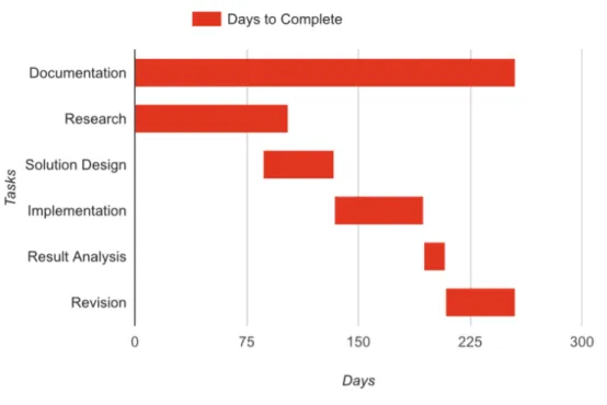
The development of this dissertation evolved through a set of well-defined stages that are shown if the figure 1. It is important to note that there is a constant awareness about the iterative nature of this process that may result in changes of the duration in each stage. At this moment, the literature review is complete and the architecture of the system is being defined. The work is being performed according to the plan (the kickoff of the project was at the beginning of October 2015).
1.6 document structure
This document will be divided into 6 chapters where the first chapter, the current one, describes all the motivations for the development of the project and what this project pro-poses to offer at its final stage, as well as, the steps outlined for this process and the type of research that was used as a guideline.
The second chapter describes the analysis made to the state of the art, in which are included an overview over the Big Data scene and the current challenges. In each section,
Figure 1.: Work plan showing the timeline of the set of tasks in this dissertation.
there will be an description of the steps of the data pipeline, and relevant findings on each topic. The most used tools will be introduced and a comparative analysis will be made, as it will serve as a basis for the following steps of this work. An introduction to the tool MongoDB aswell as a critical analysis is also part of this chapter. The last section provides an overview of Big Data projects on a wide set of areas.
The third chapter introduces the problem. By describing the architecture of the sys-tem through adequated documentation the reasinong about the contextual needs becomes simpler. The gathered needs are then discussed and quantified, the requirements are estab-lished.
In the fourth chapter the improvemetns to the system are discussed and introduced to the reader. The important and unique aspects of the setup are described. Additionally, the testing methodology is presented along with the obtained results. Some additional details are included in order to give helpful hints to those who work with this or similar systems in the future.
A careful analysis on the data collected and the results accomplished is made on the fifth chapter. The results are evaluated and compared. The discussion is made around possible explanations for the observed results and possible improvements on the testing setup. In this chapter valuable conclusions are infered that enable the orientation of data decisions on Performetric.
In the last chapter, it is put together a review of all the work developed and the results obtained. Furthermore, the future work that can be done to improve this platform and to better validate the results is indicated.
2
S TAT E O F T H E A R T
Big Data refers to things one can do at a large scale that cannot be done at a a smaller one: to extract new insights or create new forms of value, in ways that change markets, organi-zations, the relationship between citizens and governments, and moreMayer-Sch¨onberger and Cukier (2013). Despite still being somewhat an abstract concept it can be clearly said that Big Data encomprises the a new generation of technologies and architectures, designed to economically extract value from very large volumes of a wide variety of data, by enabling the high-velocity capture, discovery and analysisGantz and Reinsel(2011).
The continuous evolution of Big Data applications has brought advances in architectures used in the data centers. Sometimes these architectures are unique and have specific solu-tions for storage, networking and computing solusolu-tions regarding the particular contextual needs of the underlying organization. Therefore, when analysing Big Data we should fol-low a top down approach avoiding the risk of losing focus on the initial topic. Hence, this revision of the state of the art will be structured acording to the value chain of big data Chen et al. (2014) and its contents will be conditioned by the contextual needs evidenced by Performetric’s system. The value chain of big data can be generally divided into four phases: data generation, data acquisition, data storage, and data analytics. This approach is similar to the one that is shown it the figure2Bertino et al.(2011). Each of the first four phases of the presented pipeline can be matched with one of the phases of the Big Data value chain. For each phase the main concepts, techniques, tools and current challenges will be introduced and discussed. As it is expressed in the figure 2, there are needs that are common to all phases these include, but are not limited to: data representation, data compression (redudancy reduction), data confidentiality and energy management Bertino et al.(2011);Chen et al.(2014).
2.1 data generation and data acquisition
Data is being generated in a wide set of fields. The main sources are enterprise operational and trading data, sensor data (Internet of Things), human-computer interaction data and data generated from scientific research.
Figure 2.: The Big Data analysis Pipeline according toBertino et al.(2011).
Enterprise data is mainly data stored in traditional RDBMSs and it is related to produc-tion, inventory, sales, and financial departments and, in addition to this, there is online trading data. It is estimated that the business data volume of all companies in the world may double around every year (1.2 years according to Manyika et al.(2011)). The datasets that are a product of scientific applications are also part of the Big Data. Research in areas like bio-medical applications, computational biology, high-energy physics (for example the Large Hadron Collider) and behavior analysis (such as in Kandias et al.(2013)) generates data at an unprecedented rate.
Sensor applications, commonly known as part of the Internet of things is also a big source of data that needs to be processed. Sensors and tiny devices (actuators) embedded in physical objects—from roadways to pacemakers—are linked through wired and wireless networks, often using the same Internet Protocol (IP) that connects the InternetChui et al. (2010). Typically, this kind of data may contain redudancy (for example data streams) and has strong time and space correlation (every data acquisition device are placed at a specific geographic location and every piece of data has time stamp). The domains of application are as diverse as industry Da Xu et al. (2014), agriculture Ruiz-Garcia et al. (2009), traffic Gentili and Mirchandani(2012) and medical careDishongh et al.(2014).
Two important challenges rise regarding data generation, particularly regarding the vol-ume of and the heterogeneity. The first challange is about dealing with the fact that a significant amount of data is not relevant due to redudancy, and thus having the possibility
of being filtered and compressed by orders of magnitude. Defining the filters and being able to do so online (in order to reduce data sizes from data streams) are the main ques-tions regarding this challenge. The second challenge is to automate the generation of right metadata in order to describe what data is recorded and how it is recorded and measured as the value of data explodes when it can be linked with other dataBertino et al.(2011). 2.1.1 Data Collection
According to the International Data Corporation (IDC) the collected data can be organized in three types:
STRUCTURED DATA This type describes data which is grouped into a relational scheme (e.g., rows and columns within a standard database).
SEMI-STRUCTURED DATA : This is a form of structured data that does not conform to an explicit and fixed schema. The data is inherently self-describing and contains tags or other markers to enforce hierarchies of records and fields within the data. Examples include weblogs and social media feedsBuneman(1997).
UNSTRUCTURED DATA This type of data consists of formats which cannot easily be indexed into relational tables for analysis or querying. Examples include images, audio and video files.
As it was previously introduced, data can be acquired in a wide set of domains and through different techniques. Record files automatically generated by the system or log files are used in nearly all digital devices. Web servers, for example, record navigation data such as number of clicks, click rates, number of visits, number of unique visitors, visit durations and other properties of web users Wahab et al. (2008). The following are examples of log storage formats: NCSA, W3C Extended (used by Microsoft IIS 4.0 and 5.0), WebSphere Application Server Logs, FTP Logs.1
Another category of collected data is sensor data. Sensors are common in daily life to measure physical quantities and transform physical quantities into readable digital signals for subsequent processing (and storage). In recent years wireless sensor networks (WSN) emerged as a data sensing architechture. In a WSN, each sensor node is powered by a bat-tery and uses wireless communications. The sensor node is usually small in size and can be easily attached to any location without causing major disturbances on the surrounding environment. Examples are across wildlife habitat monitoring, environmental research, vol-cano monitoring, water monitoring, civil engineering and wildland fire forecast/detection Wang and Liu(2011).
Methods for acquiring network data such as web crawlers (program used by search en-gines for downloading and storing web pages) are also widely used for data collection. Specialized network monitoring software like Wireshark2and SmartSniff3are also used in this context.
2.1.2 Data Pre-processing
In order to improve the data analysis process, a set of techniques should be used. These are part of the data pre-processing stage and have the objective of dealing with noise in data, redudancy and consistency issues (i.e. data quality). Data integration is a mature research field in the database research community. Data warehousing processes, namely ETL (Ex-tract, Transform and Load) are the most used for data integration. Extraction is the process of collecting data (selection and analysis of sources). Transformation is the definition of a series of data flows that transform and integrate the extracted data into the desired formats. Loading means importing the data resulting from the previous operation into the target storage infrastructure. In order to deal with inacurate and incomplete data, data cleaning procedures may take place. Generally these are associated with the following complemen-tary procedures: defining and determining error types, searching and identifying errors, correcting errors, documenting error examples and error types, and modifying data acqui-sition procedures to reduce future errors Maletic and Marcus (2000). Classic data quality problems mainly come from software defects or system misconfiguration. Data redundancy means an increment of unnecessary data transmission resulting in waste of storage space and possibly leads to data inconsistency. Techniques like redundancy detection, data filter-ing, and data compression can be used in order to deal with data redudancy, however its usage should be carefully weighted as it requires extra processing power.
2.2 data storage
Big data brings more strict requirements on how data is stored and managed. This section will elaborate on the developments in different (technological) fields making big data data possible. Cloud computing, distributed file systems and NoSQL databases. A comparision based on quality attributes of the different NoSQL solutions is hereby presented.
2 https://www.wireshark.org
2.2.1 Cloud Computing
The rise of the cloud plays a significant role in big data analytics as it offers the demanded computing resources when needed. This translates to a pay for use stategy that enables the use of resources on a short-term bases (e.g. more resources on peak hours). Addition-ally there is no need for a upfront commitment about the allocated resources: users can start small but think big. Improved avalilability is another big advantage of cloud solu-tions. Clouds vary significantly in their specific technologies and implementation, but of-ten provide infrastructure (IaaS), platform (PaaS), and software resources as services (SaaS) Assunc¸˜ao et al. (2015). Cloud solutions may be private, public or hybrid (additional re-sources from a public Cloud can be provided as needed to a private Cloud). A private Cloud is suitable for organizations that require data privacy and security. Typically are used by large organizations as it enables resource sharing across the different departments. Public clouds are deployed off-site over the Internet and available to the general public, offering high efficiency and shared resources with low cost. The analytics services and data management are handled by the provider and the quality of service (e.g. privacy, security, and availability) is specified in a contract. The most popular examples of IaaS are: Amazon EC2, Windows Azure, Rackspace, Google Compute Engine. Regarding PaaS, AWS Elastic Beanstalk, Windows Azure, Heroku, Force.com, Google App Engine, Apache Stratos, are among the most widely used.
2.2.2 Distributed File Systems
An important feature of public cloud servers and Big Data systems is its file system. The most popular example of a DFS is Google File System (GFS), which as the name sugests is a proprietary system, designed by Google. Its main design features are effeciency and reliable access to data and it is designed to run on large clusters of commodity servers Zhang et al.(2010). In GFS, files are divided into chunks of 64 megabytes, and are usually appended to or read and only extremely rarely overwritten or shrunk. Compared with traditional file systems, GFS design differences are on the fact that it is designed to deal with extremely high data throughputs, provide low latency and to survive to individual server failures. The Hadoop Distributed File Systems (HDFS)4 is inspired by GFS. It is also designed to achieve reliability by replicating the data across multiple servers. Data nodes comunicate with each other to rebalance data distribution, to move copies around, and to keep the replication of data high.
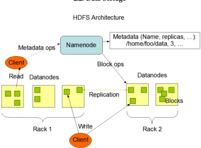
HDFS has a master/slave architecture (see figure3). An HDFS cluster consists of a single NameNode, a master server that manages the file system namespace and regulates access
Figure 3.: HDFS Architecture fromhttps://hadoop.apache.org/docs/r1.2.1/hdfs_design.html.
to files by clients. Additionaly, in the nodes of the cluster there are a number of DataNodes, usually one per node in the cluster. Data Nodes manage storage attached to the nodes that they run on. Internally, a file is split into one or more blocks and these blocks are stored in a set of DataNodes. The functions of the NameNode are to execute file system namespace operations like opening, closing, and renaming files and directories. The NameNode also determines the mapping of file ablocks to DataNodes. The DataNodes are responsible for serving read and write requests from the file system’s clients. The DataNodes also perform block creation, deletion, and replication upon instruction from the NameNode. The NameNode is the broker and the repository for all HDFS metadata. The existence of a single NameNode in a cluster simplifies the architecture of the system. One benefit of this distributed design is that user data never flows through the NameNode, so there is not a single point of failure.
2.2.3 CAP Theorem
The CAP theorem states that no distributed computing system can fulfill all three of the following properties at the same time Gilbert and Lynch(2002):
CONSISTENCY means that each node always has the same view of the data.
AVAILABILITY every request received by a non-failing node in the system must result in a response.
PARTITION TOLERANCE the system continues to operate despite arbitrary message loss or failure of part of the system (the system works well across physical network parti-tions).
Since consistency, availability, and partition tolerance can not be achieved simultaneously, we can classify existing systems into: CA systems (by ignoring partition tolerance), a CP sys-tem (by ignoring availability), and an AP syssys-tem (ignores consistency), selected according to different design goals.
2.2.4 NoSQL - Not only SQL
The term NoSQL was introduced in 1998 by Carlo Strozzi to name his RDBMS, Strozzi NoSQL (a solution that did not expose a SQL interface - the standard for RDBMS), but it was not until the Big Data era that the term became a mainstram defintion in the database world. Convetional relational databases have proven to be highly efficient, reliable and consistent in terms of storing and processing structered dataKhazaei et al.(2015). However, regarding the 3 V’s of big data the relational model has serveral shortcomings. Companies like Amazon, Facebook and Google started to work on thein own data engines in order to deal with their Big Data pipeline, and this trend inspired other vendors and open source communities to do similarly for other use cases. As Sonebraker argues in Stonebraker (2010) the main reasons to adopt NoSQL databases are performance (the ability to manage distributed data) and flexibility (to deal with semi-structured or unstructured data that may arise on the web) issues.
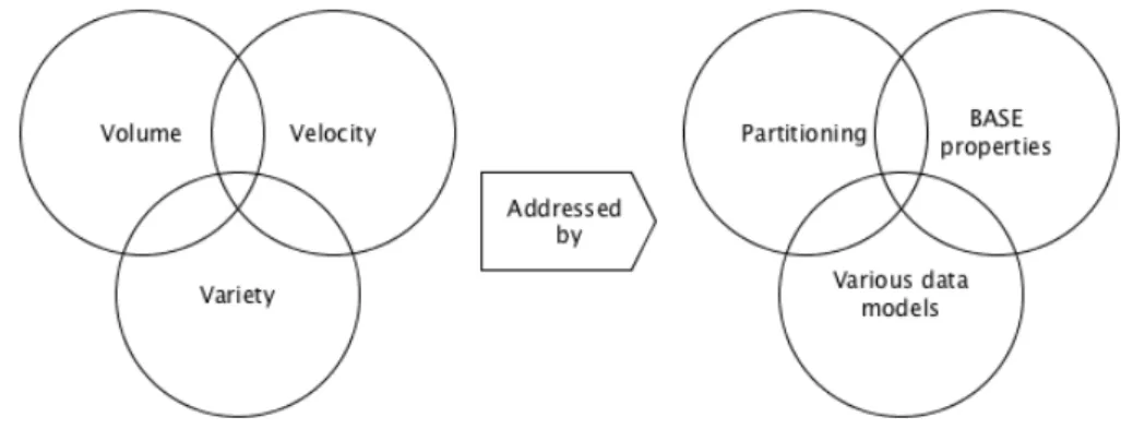
Figure 4.: Mapping between Big Data 3 V’s and NoSQL System features.
In figure4we can see a mapping between Big Data characteristics (the 3V’s) and NoSQL features that address them. NoSQL data stores can manage large volumes of data by en-abling data partitioning across many storage nodes and virtual structures, overcoming tra-ditional infrastructure constrains (and ensuring basic availability). By compromising on ACID (Atomicity, Consistency, Isolation, Durability ensured by RDBMS in database trans-actions) properties NoSQL opens the way for less blocking between user queries. The altenative is the BASE system Pritchett (2008) that translates to basic availabilty, soft state and eventual consistency. By being basically available the system is guaranteed to be mostly
available, in terms of the CAP theorem. Eventual consistency indicates that given that the system does not receive input during an interval of time, it will become consistent. The soft state propriety means that the system may change over time even without input. According toCattell(2011), the key characterisitcs that generally are part of NoSQL systems are:
1. the ability to horizontally scale CRUD operations throughput over many servers, 2. the ability to replicate and to distribute (i.e.,partition or shard) data over many servers, 3. a simple call level interface or protocol (in contrast to a SQL binding),
4. a weaker concurrency model than the ACID transactions of most relational (SQL) database systems,
5. efficient use of distributed indexes and RAM for data storage, and 6. the ability to dynamically add new attributes to data records.
However, the systems differ in many points, as the funcionality ranges from a simple distributed hashing (as supported by memcached5, an open source cache), to highly scalable partitioned tables (as supported by Google’s BigTable Chang et al. (2008)). NoSQL data stores come in many flavors, namely data models, and that permits to accommodate the data variety that is present in real problems.
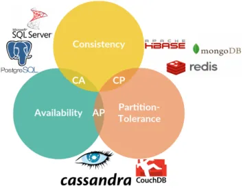
Figure 5.: Classification of popular DBMSs according to the CAP theorem.
As it shown in figure5, regarding the CAP theory, NoSQL (and relational) can be divided in CP and AP (from the CAP theorem), with CA being the relational DBMSs. Examples
of CP systems (that compromise availability) are Apache HBase6, MongoDB7 and Redis8. On the other side, favouring availability and partition-tolerance over consistency (AP) there is Apache Cassandra9, Apache CouchDB10 and Riak11. Another criterion widely used to classify NoSQL databases is based on the supported data model. According to this, we can divide the systems in the following categories: Key-value stores, document stores, graph databases and wide column stores.
Key-value Stores
The simplest form of database management systems are these. A Key-value DBMS can only perform two operations: store pairs of keys and values, and retrieve the stored values given a key. These kind of systems are suitable for applications with simple data models that require a resource-efficient data store like, for example, embedded systems or applications that require a high performance in-process database.
Memcached12Fitzpatrick(2004) is a high-performance, distributed, memory object caching system, originally designed to speed up web applications by reducing database load. Mem-cached has features similar to other key-value stores: persistence, replication, high availabil-ity, dynamic growth, backups and so on. In Memcached the identification of the destination server is done at the client side using a hash function on the key. Therefore, the architecture is inherently scalable as there is no central server to consult while trying to locate values from keys Jose et al. (2011). Basically, Memcached consists of a client software, which is given a list of available memcached servers and a client-based hashing algorithm, which chooses a server based on the “key” input. On the server side, there is an internal hash table that stores the values with their keys and an a set of algorithms that determine when to throw out old data or reuse memory.
Another example of a key-value store is Redis (REmote DIctionary Server). Redis is an in-memory database where complex objects such as lists and sets can be associated with a key. In Redis, data may have customizable time-to-live (TTL) values, after which keys are removed from memory. Redis uses locking for atomic updates and performs asynchronous replications Khazaei et al.(2015). Redis performs very well compared to writing the data into the disk for any changes in the data, in applications that do not need durability of data. As it is in-memory database, Redis might not be the right option for data-intensive
6 https://hbase.apache.org 7 https://www.mongodb.com 8 http://redis.io 9 http://cassandra.apache.org 10 http://couchdb.apache.org 11 http://docs.basho.com/riak/latest/ 12 http://memcached.org
applications with dominant read operations, because the maximum Redis data set cant be bigger than memory13.
Document-oriented Databases
Document-oriented databases are, as the name implies, data stores designed to store and manage documents. Typically, these documents are encoded in standard data exchange formats such as XML, JSON (Java Script Option Notation), YAML (YAML Ain’t Markup Language), or BSON (Binary JSON). These kind of stores allow nested documents or lists as values as well as scalar values, and the attribute names are dynamically defined for each document at runtime. When comparing to the relational model, we can say that a single column can hold hundreds of attributes, and the number and type of attributes recorded can vary from row to row, since its schema free. Unlike key-value stores, these kind of stores allows to search on both keys and values, and support complex keys and secondary indexes.
Apache CouchDB14 is a flexible, fault-tolerant database that stores collections, forming a richer data model compared to similar solutions. This solution supports as data formats JSON and AtomPub15. Queries are done with what CouchDB calls “views”, which are the primary tool used for querying and reporting, defined with Javascript to specify field con-straints. Views are built on-demand to aggregate, join and report on database documents. The indexes are B-trees, so the results of queries can be ordered or value ranges. Queries can be distributed in parallel over multiple nodes using a map-reduce mechanism. How-ever, CouchDBs view mechanism puts more burden on programmers than a declarative query languageFoundation(2014).
MongoDB16 is a database that is half way between relational and non-relational systems. Like CouchDB, it provides indexes on collections, it is lockless and it provides a query mechanism. However, there are some differences: CouchDB provides multiversion concur-rency control while MongoDB provides atomic operations on fields; l MongoDB supports automatic sharding by distributing the load across many nodes with automatic failover and load balancing, on the other hand CouchDB achieves scalability through asynchronous replication Khazaei et al. (2015). MongoDB supports master-slave replication with auto-matic failover and recovery. The data is stored in a binary JSON-like format called BSON that supports boolean, integer, float, date, string and binary types. The communication is made over a socket connection (in CouchDB it is made over an HTTP REST interface).
13 http://redis.io/documentation 14 http://couchdb.apache.org
15 http://bitworking.org/projects/atom/rfc5023.html 16 https://www.mongodb.com
Graph-oriented Databases
Graph databases are data stores that employ graph theory concepts. In this model, nodes are entities in the data domain and edges are the relationship between two entities. Nodes can have properties or attributes to describe them. These kind of systems are used for implementing graph data modeling requirements without the extra layer of abstraction for graph nodes and edges. This means less overhead for graph-related processing and more flexibility and performance.
Neo4j17 is the most known and used graph storage project. It has various native APIs in most of programming languages such as Java, Go, PHP, and others. Neo4j is fully ACID compatible and schema-free. Additionally, it uses its own query language called Cypher that is inspired by SQL, and supports syntax related to graph nodes and edges. Neo4j does not allow data partiitioning, and this means that data size should be less than the capacity of the server. However, it supports data replication in a master-slave fashion which ensures fault tolerance against server failures.
Column-oriented Databases
Column-oriented databases are the kind of data store that most resembles the relational model on a conceptual level. They retain notions of tables, rows and columns, creating the notion of a schema, explicit from the client’s perspective. However, the design princi-ples, architecture and implementation are quite different from traditional RDBMS. While the notion of tables’ main function is to interact with clients, the storage, indexing and dis-tribution of data is taken care by a file and a management system. In this approach, rows are split across nodes through sharding on the primary key. They typically split by range rather than a hash function. This means that queries on ranges of values do not have to go to every node. Columns of a table are distributed over multiple nodes by using “column groups”. These may seem like a new complexity, but column groups are simply a way for the customer to indicate which columns are best stored together Cattell(2011). Rows are analogous to documents: they can have a variable number of attributes (fields), the attribute names must be unique, rows are grouped into collections (tables), and an individual row’s attributes can be of any type. For applications that scan a few columns of many rows, they are more efficient, because this kind of operations lead to less loaded data than reading the whole row. Most wide-column data store systems are based on a distributed file system. Google BigTable, the precursor of the popular data store systems of this kind, is built on top of GFS (Google File System).
Apache HBase is the NoSQL wide-column store for Hadoop, the open-source implemen-tation of MapReduce for Big Data analytics. The purpose of HBase is to support random,
real-time read and write access to very large tables with billions of rows and millions of columns. HBase uses the Hadoop distributed file system in place of the Google file system. It puts updates into memory and periodically writes them out to files on the disk. Row operations are atomic, with row-level locking and transactions. Partitioning and distribu-tion are transparent; there is no client-side hashing or fixed keyspace as in some NoSQL systems. There is multiple master support, to avoid a single point of failure. MapReduce support allows operations to be distributed efficiently.
Apache Cassandra is designed under the premise that failures may happen both in soft-ware and hardsoft-ware, being practically inevitable. It has column groups, updates are cached in memory and then flushed to disk, and the disk representation is periodically compacted. It does partitioning and replication. Failure detection and recovery are fully automatic. However, Cassandra has a weaker concurrency model than some other systems: there is no locking mechanism, and replicas are updated asynchronously.
Comparative Evaluation of NoSQL Databases
As it was presented, there are several options when it comes the time to choose a NoSQL database, and the different categories and architectures serve different purposes. Although four categories were presented, only two of them are adequate for the purposes of this work. Regarding support for complex queries column-oriented and document-oriented data store systems are more adequate than key-value stores (e.g. simple hash tables) and graph databases (which are ideal for situations that are modeled as graph problems). Con-sidering the last presented fact, we selected Apache Cassandra, CouchDB, Apache HBase and MongoDB as the object of this evaluation. The following table is based in the work presented in Lourenc¸o et al. (2015), where several DBMS are classified in a 5-point scale (Great, good, average, mediocre and bad) regarding a set of quality atributes.
DBMS Cassandra CouchDB HBase MongoDB
Availability Great Great Mediocre Mediocre
Consistency Great Good Average Great
Durability Mediocre Mediocre Good Good Maintainability Good Good Mediocre Average Read-Performance Good Average Mediocre Great
Recovery Time Great Unknown Unknown Great
Reliability Mediocre Good Good Great
Robustness Good Average Bad Average
Scalability Great Mediocre Great Mediocre Stabilization Time Bad Unknown Unknown Bad Write-Performance Good Mediocre Good Mediocre
As it is mentioned inLourenc¸o et al.(2015), the follwing criteria were used:
AVAILABILITY the downtime was used as a primary measure, together with relevant studies such as Nelubin and Engber(2013).
CONSISTENCY was graded according to how much the database can provide ACID-semantics and how much can consistency be fine-tuned.
DURABILITY was measured according to the use of single or multi version concurrency control schemes, the way that data are persisted to disk (e.g. if data is always asyn-chronously persisted, this hinders durability), and studies that specifically targeted durability.
MAINTAINABILITY the currently available literature studies of real world experiments, the ease of setup and use, as well as the accessibility of tools to interact with the database. READ AND WRITE PERFORMANCE the grading of this point was done by considering recent
studies (Nelubin and Engber(2013)) and the fine-tuning of each database. RELIABILITY is graded by looking at synchronous propagation modes.
ROBUSTNESS was assessed with the real world experiments carried by researchers, as well as the available documentation on possible tendency of databases to have problems dealing with crashes or attacks.
SCALABILITY was assessed by looking at each database’s elasticity, its increase in perfor-mance due to horizontal scaling, and the ease of live addition of nodes.
STABILIZATION AND RECOVERY TIME this measure is highly related to availability and is based our classification on the results shown inNelubin and Engber(2013).
Although there have been a variety of studies and evaluations of NoSQL technology, there is still not enough information to verify how suited each non-relational database is in a specific scenario or system. Moreover, each working system differs from another and all the necessary functionality and mechanisms highly affect the database choice. Sometimes there is no possibility of clearly stating the best database solution Lourenc¸o et al.(2015). 2.3 data analytics
Data analytics encomprises the set of complex procedures running over large-scale, data repositories (like big data repositories) whose main goal is that of extracting useful knowl-edge kept in such repositories Cuzzocrea et al. (2011). Along with the storage problem (conveying big data stored in heterogeneous and different-in-nature data sources into a
structured format), the issue of processing and transforming the extracted structured data repositories in order to derive Business Intelligence (BI) components like diagrams, plots, dashboards, and so forth, for decision making purposes, is the most addressed aspect by organizations.
In this section, one of the most widely used tool for data aggregation, Hadoop MapRe-duce Framework18 (and its programming modet that enables parallel and distributed data processing) is introduced, alongside with its architecture. MongoDB Aggregation Frame-work is also introduced as it provides a recent and different approach by providing a tool for data aggregation contained in the database environment. Additionally, the concept of Real-time analytics is explored and examples of supporting tools are provided.
2.3.1 MapReduce
MapReduce is a scalable and fault-tolerant data processing tool that enable the processing of massive volumes of data in parallel with many low-end computing nodes Lee et al. (2012). In the context of Big Data analytics, MapReduce presents an interesting model where data locality is explored to improve the performance of applications. The main idea of the MapReduce model is to hide details of parallel execution, allowing the users to focus on data processing strategies. MapReduce utilizes the GFS while Hadoop MapReduce, the popular open source alternative, runs above the HDFS.
The computation takes a set of input key/value pairs, and produces a set of output key/value pairs. The MapReduce model consists of two primitive functions: Map and Reduce. Map, written by the user, takes an input pair and produces a set of intermediate key/value pairs. The MapReduce library groups together all intermediate values associated with the same intermediate key and passes them to the Reduce function. The Reduce function accepts an intermediate key and a set of values for that key. It merges together these values to form a possibly smaller set of values. Typically just zero or one output value is produced per Reduce invocation. The intermediate values are supplied to the user’s reduce function via an iterator. This allows the handling of lists of values that are too large to fit in memory Dean and Ghemawat(2008). The following example (see figure7) is about the problem of counting the number of occurrences of each word in a large collection of documents.
18 https://hadoop.apache.org/docs/current/hadoop-mapreduce-client/hadoop-mapreduce-client-core/ MapReduceTutorial.html
Figure 6.: Hadoop MapReduce architecture.
map ( String key , String value ) : // key : d o c u m e n t name
// value : d o c u m e n t c o n t e n t s for each word w in value :
E m i t I n t e r m e d i a t e (w , " 1 " ) ;
reduce ( String key , I ter ato r values ) : // key : a word
// values : a list of counts int result = 0;
for each v in values : result += P ars eIn t ( v ) ; Emit ( A sSt rin g ( result ) ) ;
Figure 7.: Pseudocode representing a words counting implementation in map-reduce. The main advantages of using MapReduce are its simplicity and ease of use, being storage independent (can work with different storage layers), its fault tolerance and providing high-scalability. On the other hand, there are some pitalls, such as: the lack of a high-level language, being schema-free and index-free, lack of maturity and the fact that operations not being always optimized for I/O efficiency. Lee et al.(2012).
2.3.2 Real Time Analytics
In the spectrum of analytics two extremes can be identified. On one end of the spectrum there is batch analytical applications, which are used for complex, long-running analyses. Generally, these have slower response times (hours or days) and lower requirements for availability. Hadoop-based workloads are an example of batch analytical applications. On the other end of the spectrum sit real-time analytical applications. Real-time can be consid-ered from the point of view of the data or from the point of view of the end-user. The earlier translates into the ability of processing data as it arrives, making it possible to aggregate data and extract trends about the actual situation of the system (streaming analytics). The former refers to the ability to process data with low latency (processing huge amount of data with the results being available for the end user almost in real-time) making it possible, for example, to to provide recommendations for an user on a website based on its history or to do unpredictable, ad hoc queries against large data sets (online analytics).
Regarding stream processing the main problems are related to: Sampling Filtering, Cor-relation, Estimating Cardinality, Estimating Quantiles, Estimating Moments, Finding Fre-quent Elements, Counting Inversions, Finding Subsequences, Path Analysis, Anomaly De-tection Temporal Pattern Analysis, Data Prediction, Clustering, Graph analysis, Basic Count-ing and Significant CountCount-ing. The main applications are A/B testCount-ing, set membership, fraud detection, network analysis, traffic analysis, web graph analysis, sensor networks and medical imaging (Kejariwal et al.(2015)).
According toKejariwal et al.(2015) these are the most well-known streaming open source tools:
S4 Real-time analytics with a key-value based programming model and support for schedul-ing/message passing and fault tolerance.
STORM The most popular and widely adopted real-time analytics platform developed at Twitter.
MILLWHEEL Google’s proprietary realtime analytics framework thats provides exact once semantics.
SAMZA Framework for topology-less real-time analytics that emphasizes sharing between groups.
AKKA Toolkit for writing distributed, concurrent and fault tolerant applications. SPARK Does both offline and online analysis using the same code and same system. FLINK Fuses offline and online analysis using traditional RDBMS techniques. PULSAR Does real-time analytics using SQL.
HERON Storm re-imagined with emphasis on higher scalability and better debuggability. Online analytics, on the other hand, are designed to provide lighter-weight analytics very quickly. The requirements of this kind of analytics are low latency and high availability. In the Big Data era, OLAP (on-line analytical processing Chaudhuri and Dayal (1997)) and traditional ETL processes are too expensive. Particularly, the heterogeniety of the data sources difficults the definition of rigid schemas, making model-driven insight difficult. In this paradigm analytics are needed in near real time in order to support operational applications and their users. This includes applications from social networking news feeds to analytics, from real-time ad servers to complex CRM applications.
2.3.3 MongoDB Aggregation Framework
MongoDB is actually more than a data storage engine, as it also provides native data pro-cessing tools: MapReduce19and the Aggregation pipeline20. Both the aggregation pipeline and map-reduce can operate on a sharded collection (partitioned over many machines, hor-izontal scaling). These are powerful tools for performing analytics and statistical analysis in real-time, which is useful for ad-hoc querying, pre-aggregated reports, and more. Mon-goDB provides a rich set of aggregation operations that process data records and return computed results, using this operations in the data layer simplifies application code and limits resource requirements. The documentation of MongoDB provides a comparison of the different options of aggregation commands21.
The Aggregation pipeline (introduced in MongoDB 2.2) is based on the concept of data processing pipelines (analogous to the unix pipeline). The documents are processed in a multi-stage pipeline that produces the aggregated results. Each stage transforms the doc-uments as they pass through the pipeline. Output of first operator will be fed as input to the second operator and so on. Despite, being limited to the operators and expressions sup-ported, the aggregation pipeline can add computed fields, create new virtual sub-objects, and extract sub-fields into the top-level of results by using the project22pipeline operator.
Follwing the pipeline architecture pattern, expressions can only operate on the current document in the pipeline and cannot refer to data from other documents: expression op-erations provide in-memory transformation of documents. Expressions are stateless and are only evaluated when seen by the aggregation process with one exception: accumulator expressions. The accumulators, used in the group23 stage of the pipeline, maintain their state (e.g. totals, maximums, minimums, and related data) as documents progress through
19 https://docs.mongodb.org/manual/core/map-reduce/
20 https://docs.mongodb.org/manual/core/aggregation-pipeline/
21 https://docs.mongodb.org/manual/reference/aggregation-commands-comparison/
22 https://docs.mongodb.org/manual/reference/operator/aggregation/project/#pipe._S_project 23 https://docs.mongodb.org/manual/reference/operator/aggregation/group/#pipe._S_group
Figure 8.: MongoDB Aggregation Pipeline example.
the pipeline. In version 3.2 (the most recent) some accumulators are available in the project stage, but it this situation they do not maintain their state across documents.
2.4 machine learning
In this section, an introduction to the current state of machine learning will be provided. This review will follow a top-down approach. The basic concepts of learning will be intro-duced, and further in the section an overview of deep neural networks (the main theoretical topic driving machine learning research) will be presented, essentialy from a user perspec-tive. The goal here is to provide insight on how the current machine learning techniques are located in the big data scene, what to expect from them in the near future and how could they help to provide real-time intelligence.
2.4.1 Introduction to Learning
A computer program is said to learn from experience E with respect to some class of tasks T and performance measure P if its performance at tasks in T, as measured by P, improves with experience E (Mitchell (1997)). From this formal definition of machine learning, a generalization can be made categorizing such systems as systems that automatically learn
programs from data (Domingos (2012)). As the data volumes grow rapidly this premise becomes more and more attractive, providing alternative to manually constructing the de-sired programs. Among other domains Machine learning is used in Web search, spam filters, recommender systems, ad placement, credit scoring, fraud detection, stock trading, drug design, among others.
Generally, learning algorithms consist of combinations of just three components. For each of the components the list of options is very large resulting in a variety of machine learning algorithms that is in the order of magnitude of the thousands. The three components are described below (Domingos(2012)):
REPRESENTATION A classifier must be represented in some formal language that the com-puter can handle. Conversely, choosing a representation for a learner is equivalent to choosing the set of classifiers that it can possibly learn. This set is called the hypoth-esis space of the learner. The crucial question at this stage is how to represent the input, i.e., what features to use.
EVALUATION An evaluation function (also called objective function or scoring function) is needed to distinguish good classifiers from bad ones. Examples of evaluation func-tions are: accuracy/error rate, precision and recall, squared error, and likelihood.
OPTIMIZATION a method to search among the classifiers in the language for the highest-scoring one. The choice of optimization technique is key to the efficiency of the learner, and also helps determine the classifier produced if the evaluation function has more than one optimum. The optimization methods are can be combinatorial (greedy search, beam search, branch-and-bound) or continuous (gradient descent, quasi-newton methods, linear and quadratic programming).
Many different types of machine learning exist, such as clustering, classification, regres-sion and density estimation. There is a fundamental difference on the types of algorithms that is related to goals of the learning process. In order to illustrate these differences, the definitions of clustering (unsupervised learning) and classification (supervised learning) are hereby presented (Bagirov et al.(2003)).
Clustering names the process of identification of subsets of the data that are similar between each other. Intuitively, a subset usually corresponds to points that are more similar to each other than they are to points from another cluster. Points in the same cluster are given the same label. Clustering is carried out in an unsupervised way by trying to find subsets of points that are similar without having a predefined notion of the labels.
Classification, on the other hand, involves the supervised assignment of data points to predefined and known classes. It is the most mature and widely used type of machine learning. In this case, there is a collection of classes with labels and the goal is to label a new observation or data point as belonging to one or more of the classes. The known classes of examples constitute a training set and are used to learn a description of the classes (determined by some a priori knowledge about the dataset). The trained artifact can then be used to assign new examples to classes.
Another definition that is relevant in this context is the concept of reinforcement learn-ing, that is much more focused on goal-directed learning from interaction than are other approaches to machine learning. Reinforcement learning is a formal mathematical frame-work in which an agent manipulates its environment through a series of actions, and in response to each action, receives a reward value. An agent stores its knowledge about how to choose reward-maximizing actions in a mapping form agent-internal states to actions. In essence, the agent’s “task” is to maximize reward over time. Good task performance is precisely and mathematically defined by the reward values (McCallum(1996)).
The goal of these kind of algorithms is to obtain a generalization, however no matter how much data is available, data alone is not enough. Every learner must embody some knowledge or assumptions beyond the data it’s given in order to generalize beyond it. This was formalized by Wolpert in his famous “no free lunch” theorems, according to which no learner can beat random guessing over all possible functions to be learned (Wolpert(1996)).
The catch here is the fact that the functions to be learned in the real world are not drawn uniformly from the set of all mathematically possible functions. In fact, very general assumptions are often enough to do very well, and this is a large part of why machine learning has been so successful.
The main problems associated with learning algorithms are the possibility of overfitting over the training data and the “curse” of dimensionalityBellman(1961).
Overfitting it comes in many forms that are not immediately obvious. When a learner outputs a classifier that fits all the training data but fails on most of the data from the test dataset, it has overfit. One way to understand overfitting is by decomposing generalization error into bias and variance (see figure9). Bias is a learner’s tendency to consistently learn the same wrong thing. Variance is the tendency to learn random things irrespective of the real signal. It’s easy to avoid overfitting (variance) by falling into the opposite error of underfitting (bias). Simultaneously avoiding both requires learning a perfect classifier, and short of knowing it in advance there is no single technique that will always do best (no free lunch). Generalizing correctly becomes exponentially harder as the dimensionality (number of features) of the examples grows, because a fixed-size training set covers a very small fraction of the input space. Fortunately, there is an effect that partly counteracts the curse as in most applications examples are not spread uniformly throughout the instance space,
but are concentrated on or near a lower-dimensional manifold. Learners can implicitly take advantage of this lower effective dimension, or algorithms for explicitly reducing the dimensionality can be used.
Figure 9.: Bias and variance in dart-throwing (Domingos(2012)).
In the Big Data context, data mining techniques and machine learning algorithms have been very useful in order to make use of complex data, bringing exciting opportunities. For example, researchers have successfully used Twitter to detect events such as earthquakes and major social activities, with nearly online speed and very high accuracy. In addition, the knowledge of people’s queries to search engines also enables a new early warning system for detecting fast spreading flu outbreaks (Wu et al.(2014)).
2.4.2 Deep Neural Network Architecutres
The recent vast research activities in neural classification have established that neural net-works are a promising alternative to various conventional classification methods. The ad-vantage of neural networks lies in four theoretical aspects.
• Neural networks are data driven self-adaptive methods in that they can adjust them-selves to the data without any explicit specification of functional or distributional form for the underlying model.
• They are universal functional approximators, meaning that neural networks can ap-proximate any function with arbitrary accuracy.