ISSN 1549-3636
© 2008 Science Publications
Corresponding Author: Jalal Atoum, Department of Computer Science, Princess Sumaya University For Technology, Amman-Jordan, P.O. Box 1438 Al-Jubaiha, 11941 Jordan
421
Mining Functional Dependency from Relational Databases
Using Equivalent Classes and Minimal Cover
1Jalal Atoum, 2Dojanah Bader and 1Arafat Awajan
1Department of Computer Science, PSUT, Amman, Jordan
2Amman University College, Albalqa Applied University, Amman, Jordan
Abstract: Data Mining (DM) represents the process of extracting interesting and previously unknown knowledge from data. This study proposes a new algorithm called FD_Discover for discovering Functional Dependencies (FDs) from databases. This algorithm employs some concepts from relational databases design theory specifically the concepts of equivalences and the minimal cover. It has resulted in large improvement in performance in comparison with a recent and similar algorithm called FD_MINE.
Key words: Data mining, functional dependencies, equivalent classes, minimal cover
INRODUCTION
FDs are relationships (constraints) between the attributes of a database relation; a FD states that the value of some attributes are uniquely determined by the values of some other attributes. Discovering FDs from databases is useful for reverse engineering of legacy systems for which the design information has been lost. Furthermore, discovering FDs can also help a database designer to decompose a relational schema into several relations through the normalization process to get rid or eliminate some of the problems of unsatisfactory database design. The identification of these dependencies that are satisfied by a database instance is an important topic in data mining literature[5]. The problem of generating or discovering FDs from relational databases had been studied in[3,4,7,8,11,12]. A straight forward solution algorithm is shown to require exponential time of all inputs (number of attributes and number of tuples in a relation).
In this study, we are proposing a new algorithm for discovering FDs from static databases. This algorithm will use and employ some concepts from relational database theory, such as the theory of equivalencies and minimal cover of FDs. The proposed algorithm aims at minimizing the time requirements of algorithms that discover FDs from databases. We will compare the result of our proposed algorithm with a previous well known algorithm called FD_MINE[12].
Some of the previous studies in discovering FDs from databases presented in[2,4,8] have focused on discovering embedded parallel query execution,
optimizing queries, providing some kind of summaries over large data sets or discovering association rules in stream data.
Other studies presented in[3,7,9,11,12] have presented various methods for discovering FDs from large databases, these studies have focused on discovering FDs from very large databases and had faced a general problem which is represented by the exponential time requirements that depend on database size (the dimensionality problem in number of tuples and attributes).
Functional dependencies: An FD, denoted by X→Y, is constraint between two sets of attributes X and Y that are subsets of some relation schema R. It specifies a constraint on all possible tuples t1 and t2 in R such that if t1[X] = t2[X], then they must also have t1[Y] = t2[Y]. This means that the value of the Y component in any tuple in R depend on or are determined by the value of the X component or alternatively the value of the X component of any tuple uniquely (or functionally) determines the value of the Y component.
Definition 1: If A is an attribute or set of attributes in relation R, all the attributes in R that are functionally dependent on A in relation R with respect to F (where F is a set of FDs that holds on R), form the closure of A and it is denoted by A+ or Closure(A).
Definition 3: The closure of a set F of FDs is the set of all FDs that are logically implied by F and it is denoted by F+.
Minimal cover: Minimal FDs or minimal cover is a useful concept in which all unnecessary FDs are eliminated from F. The concept of minimal cover of F is sometimes called Irreducible Set of FDs. The minimal cover of FDs of F is denoted by Fc.
To find the minimal cover of a set of FDs of F, we transform F such that for each one of its FDs that has more than one attribute in the right hand side is reduced to a set of FDs that have only one attribute on the right hand side. The minimal cover Fc is then a set of FDs such that:
• Every right hand side of each dependency is a single attribute
• For X→A in F then the set F-{X→A} equivalent to F
• For X→A in F and a proper subset Z of X is F-{X→A} U {Z→A} equivalent to F
Example 3.1, Consider the following set of FDs on schema R (A, B, C):
F = {A→BC, B→C, A→B, AB→C}
Then the Minimal Cover of F is Fc = {A→B, B→C}.
Functional dependencies and equivalent classes: To discover a set of FDs that are satisfied by a relation instance, we use the partition method that divides the tuples of this instance into groups based on the different values of each column (attribute). For each attribute, the number of groups is equal to the number of different values for that attribute. Each group is called an equivalent class[10]. For instance, given the following relation instance as shown in Table 1 that has five attributes with binary values:
For attribute A, there are two different values (0 and 1), then the tuples that have 0 are {1,2,5} and the tuples that have 1 are {3,4}. Hence, the equivalent classes for attribute A are {{1,2,5},{3,4}}. Similarly for the other attributes {B, C, D and E}, their equivalent classes are as follows respectively: {{1, 2, 3, 5}, {4}}, {{1, 2, 3, 5}, {4}}, {{1, 2, 5}, {3, 4}} and {{1, 2, 4}, {3, 5}}.
Next, we test each pair of equivalent classes of each pair of attributes if they are same or not. For each pair of equivalent classes that are the same, we conclude that their corresponding attributes are equivalent and each attribute is functionally determined
Table1: Binary relation instance
Tuple ID A B C D E
t1 0 1 0 1 0 t2 0 1 0 1 0 t3 1 1 0 0 1 t4 1 0 1 0 0 t5 0 1 0 1 1
Fig. 1: Lattice for the attributes of the relation in Table 1
by the other. For instance, since the equivalent classes for attribute A = the equivalent classes for attribute D, we can conclude that attribute A is equivalent to attribute D and consequently: (A↔D, A→D, D→A). Furthermore, A can be added to the closure of D and D can be added to the closure of A.
This process is repeated for all attributes and for all of their combinations (candidate set). For instance, given a relation with five attributes (A, B, C, D, E) the candidate set is {φ, A, B, C, D, E, AB, AC, AD, AE, BC, BD, DE, CD, CE, DE, ABC, ABD, ABE, ACD, ACE, ADE, BCD, BCE, BDE, CDE, ABCD, ABCE, ABDE, ACDE, BCDE, ABCDE} for a total of 32 (i.e., 25) combinations. These candidate attributes of this relation are represented as a lattice as shown in Fig. 1.
Each node in Fig. 1 represents a candidate attributes. An edge between any two nodes such as E and DE indicates that the FD: DE→D, needs to be checked. Hence, discovering FDs from very large databases with large number of attributes may require an exponential time[6, 8].
423
FD_M INE algorithm
To discover all functional dependencies in a dataset. Input: Dataset D and its attributes X 1, X 2, ... , X m Output: FD_SET, EQ_SET and KEY_SET {
1. Initialization step
Set R = {X1, X2, ..., Xm}, set FD_SET =∅, Set EQ_SET = ∅, set KEY_SET = ∅ Set CANDIDATE_SET = {X 1, X 2, ..., X m} For all X i ∈CANDIDATE_SET do
Set Closure'[X i] = ∅ 2. Iteration step
While CANDIDATE_SET ? ∅ do {
For all Xi∈CANDIDATE_SET do {
ComputeNonTrivialClosure(X i) ObtaintFDandKey(X i) }
ObtainEQSet(C ANDIDATE_SET) PruneCandidates(CANDIDATE_SET) GenerateCandidates(CANDIDATE_SET) }
3. Display (FD_SET, EQ_SET, KEY_SET) }
Fig. 2: The main procedure of FD_MINE algorithm
Time complexity of FD-MINE algorithm: The main body of the FD_MINE algorithm has a loop that iterates n times, where n is the cardinality of the candidate set in the given database. Therefore, this main body has a time complexity of n. Within each iteration of the above loop, there is a call for each of the following:
• A loop that iterates n times over all attributes in the Candidate_Set within each iteration of this loop there is call for each of the following procedures:
• ComputeNonTrivialClosure(), this procedure iterates n times
• ObtainFDandKey(), this procedure iterates n times. For a total time of n (n+n)= 2 n 2
• ObtainEQSet(), this procedure performs two nested loops each with n iterations for a total time of n2.
• PruneCandidates(CANDIDATE_SET. this
procedure performs one loop with n iteration.
• GenerateCandidates(CANDIDATE_SET) this procedure performs two nested loops each with n iterations for a total time of n2.
Therefore, the total time required by the FD_MINE algorithm is:
T (n) = n (2 n2+n2+n+n2) = 4n3+n2
Suggested work: In this study, we suggest an algorithm that discovers all FDs from databases that
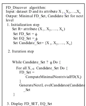
FD_Discover algorithm:
Input: dataset D and its att ribute X1,X2,….,Xn Out put: Minim al FD_Set, Candidate Set for next level
1. Initializat ion step
Set R= at tribute (X1, X2,….., Xn) Set FD_Set = φ
Set EQ_Set =φ
Set Candidat e_Set= {X1, X2,….., Xn}
2. It erat ion step
While Candidat e_Set ? φ Do {
For all Xi∈ Candidate_Set Do { FD_Set =
ComputeMinimalNontrivialFD(Xi) }
GenerateNextL evelCandidates(Candidate _Set
}
3. Display FD_SET , EQ_Set
Fig. 3: The main procedure of the FD_Discover algorithm
reduces the number of attributes and FDs to be checked. The suggested algorithm called FD_Discover and it will incorporate the following concepts.
• An incremental minimal (Canonical) cover computation during each phase of discovering FDs to minimize the number of FDs to be checked
• During each phase of the algorithm and for each attribute, we compute its nontrivial closure attributes. For each equivalent pair of attribute closures, we remove one of them from the candidate set of attributes. Also, we add the fact that these two attributes are equivalent (↔). This will reduce the number of attributes to be checked during each phase of the algorithm
FD_Discover algorithm: To introduce our FD_Discover algorithm the following terms should be defined:
EQ_Set = Set of discovered equivalent set in form: X ↔ Y.
Candidate_Se t= attributes over a dataset to be checked (Relation Attributes).
Xi: One of the attributes in candidate_set. Figure 3 shwos the main procedure of the FD_Discover algorithm.
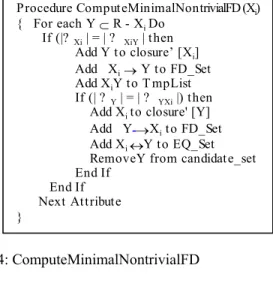
P rocedure Comput eMinimalNontrivialFD (Xi)
{ For each Y ⊂ R - Xi Do If (|? Xi | = | ? XiY | t hen
Add Y t o closure’ [Xi]
Add Xi→ Y t o FD_Set
Add XiY t o T mpList
If (| ?Y | = | ? YXi |) t hen Add Xi t o closure' [Y]
Add Y→Xi t o FD_Set Add Xi ↔Y t o EQ_Set
RemoveY from candidat e_set End If
End If Next At t ribut e }
Fig. 4: ComputeMinimalNontrivialFD
Procedure
GenerateNextLevelCandidates(CANDIDATE_SET) {
For each Xi ∈ CANDIDAT E_SET do For each Xj ∈ CANDIDAT E_SET do If (Xi[1]=Xj[1], …, Xi[k-2] = Xj[k-2] and Xi[k-1] < Xj[k-1]) then
{Set Xij = Xi join Xj
If ∃Xij∈ T mpList then delete Xij Else
Compute the partition ПXij of Xij endif
} // end procedure
Fig. 5: GenerateNextLevelCandidates (CANDIDATE_ SET)
attribute its nontrivial closure set. For each attribute Xi if Y in its closure then add Xi→Y to the FD_Set and add XiY to TmpList.
Furthermore, this procedure checks each pair of attributes whether their closures are equivalent or not. For each equivalent pair remove one of the attributes from the candidate set of attributes. Figure 5 shows the GenerateNextLevelCandidates procedure.
Example: Given the database shown in Table 1, the following steps show how our suggested algorithm can be applied on this relation only for the first level.
• Initialization step, the following identifiers would be initialized as follows:
• CANDIDATE_SET= {A, B, C, D}
• FD_SET: { }
• EQ_SET: { }
• Next, the algorithm iterates over the following steps until the candidate set is empty.
The procedure ComputeNonTrivialFD (Xi) iterates n times according to the number of attributes as follows:
n = 1, ComputeMinimalNontrivialFD(A): Since attribute (A) has two attributes in its closure set {B, D}, for each attribute in this set, this procedure first adds the fact that attribute A functionally determines each attribute in this closure set to FD_Set (i.e., FD_Set = {A→B, A→D}). Next, it checks whether attribute A is equivalent to attribute B then to attribute D. Consequently, this procedure finds out that only attribute D is equivalent to attribute A. Therefore {A→D} is added to EQ_Set and immediately it updates the Candidate_Set by removing attribute {D} from it (i.e. Candidate_Set = {A, B, C}).
Therefore, FD_Set = {A→B, A→D} and EQ_Set = {A→D}
n = 2, ComputeMinimalNontrivialFD(B): Attribute (B) has no attributes in its closure set, therefore no change to FD_Set and EQ_Set. Hence, Closure' (B) = {}, FD_Set = {A→B, A→D} and EQ_Set = {A→D}
n = 3, ComputeMinimalNontrivialFD(C): Attribute (C) has one attribute in its closure set {B}, for each attribute in this set, this procedure first adds the fact that attribute C functionally determines each attribute in its closure set to FD_Set (i.e add C→B to FD_Set. Therefore FD_Set = {A→B, A→D, C→B}). Next this procedure checks whether attribute C is equivalent to attribute B or not. This procedure finds out that attribute B is not equivalent to attribute C
Time coplexity of FD_Discover algorithm: The main body of the FD_Discover algorithm has a loop that iterates n times, where n is the cardinality of the candidate set, in the given database. Therefore, this main body has a time complexity of n. Within each iteration of the above loop, there is a call for each of the following procedures:
• ComputeMinimalNontrivialFD(), this procedure is called n times each call of this procedure takes n iterations, for a total time of n2
• GeneratNextLevelCandidates(Candidate_Set) this procedure performs two nested loops, each with n iteration for a total time of n2
Therefore, the total time required by the FD_Discover algorithm is:
425 Table 2: Actual time requirements at all level for both algorithms
(FD_MINE and the FD_Discover algorithm) for some UCI datasets
Time for Time for No. of No. of FD_Discover FD_MINE DB name attributes tuples (min) (min) Abalone 9 4,177 1.05 5.55 Balance-scale 5 625 0.003 0.04 Breast-cancer 11 699 15.21 70.05 Bridge 13 108 75.43* 410.48 Chess 7 28,056 0.14 1.07
Echocardiogram 13 132 5.55* 26.07 Glass 11 214 1.23 3.45 Iris 5 150 0.0002 0.03 Nursery 9 12,960 2.56 13.14 Machine 10 209 1.24 9.13
Table 3: Time complexity comparison based on T(n) for both algorithms
No. of Coordinate FD_MINE FD_Discover Database name attribute of datasets 2n 4n3+n2 2n3
Abalone 9 512 2997 1458 Balance-scale 5 32 525 250 Breast-cancer 11 2048 5445 2662 Bridge 13 8192 8957 4394 Chess 7 128 1421 686
Echocardiogram 13 8192 8957 4394
Glass 11 2048 5445 2662 Iris 5 32 525 250 Nursery 9 512 2997 1458 Machine 10 1024 4100 2000
RESULTS AND DISCUSSION
Table 2 shows the results of the actual times (on a PC with speed of 2.3 GHz) required for FD_MINE algorithm and FD_Discover algorithm for different UCI datasets[1] with varying number of attributes for discovering all FDs at all levels.
In Table 2 Bridge and Echocardiogram datasets have the same number of attributes and a similar number of tuples but the time required for Echocardiogram database is much less than the time required for Bridge database. This had happened because they have different data and Echocardiogram has more equivalent attributes than Bridge so the number of checks is less and the time required is also less. From these results we can notice that our FD_Discover algorithm needs less time than FD_MINE by a factor of almost 5.
Table 3 shows the time complexity comparison based on T(n) that are computed earlier for FD_Discover algorithm and for FD_MINE algorithm.
The FD_Discover algorithm reduces the number of FDs to be checked and produces fewer FDs than FD_MINE algorithm (the FDs that are discovered by the FD-Discover algorithm are equivalent to those FDs that are discovered by the FD_MINE algorithm).
ABCE
ABC ABE ACE BCE
AB AC AE BC BE CE
A B C E
(a)
ABCE ABCD ABDE
ABCDE
ACDE BCDE
ABC ABD ABE ACD ACE ADE BCD BCE BDE CDE
AB AC AD AE BC BD BECD CE DE
A B C D E
(b)
Fig. 6: Semi-lattice of checked FDs, (a): FD_Discover, (b): FD_MINE
Therefore, the Semi-lattice for FD-Discover algorithm will be smaller than the semi-lattice of FD-MINE algorithm. For instance, during the discovering process of the FDs from the database given in Table 1, Fig. 6a shows the semi-lattice of checked FDs using FD_Discover algorithm and Fig. 6b shows the semi-lattice of checked FDs using FD_MINE algorithm. It is noticed that the semi-lattice for FD_Discover algorithm has fewer edges than the semi-lattice for FD_MINE algorithm.
CONCLUSION
We have suggested a new algorithm (FD_Discover) to discover FDs which utilizes the concepts of equivalent properties and minimal (Canonical) cover of FDs.
The aim of this algorithm is to optimize the time requirements when compared with a previous algorithm called FD_MINE. The analyses of the FD_Discover algorithm had a better performance of a factor of 5 over the FD_MINE algorithm.
algorithm all attributes must be checked. In FD_Discover algorithm only one procedure (Procedure ComputeMinimalNontrivialFD) is needed to discover immediately FD_Set, EQ_Set and pruning Candidate set for next level, whereas FD_MINE algorithm needs three procedures one to discover FD_Set (ObtainFDandKey), another to discover EQ_Set (ObtainEQSet) and PruneCandidates and GenerateNextLevelCandidate to prune Candidate set for next level. This leads to higher complexity in number of nested loops and time required.
REFERENCES
1. Blake, C.L. and C.J. Merz, 1998. UCI repository of machine learning databases. Dept. of Information and Computer Science, University of California, Irvine, CA. http://www.ist-world.org/ ResultPublicationDetails.aspx?ResultPublicationId =166f0434fd5c422898e1ee4618d683f6.
2. Dorneich, A., R. Natarajan, E. Pednault and F. Tipu, 2006. Embedded predictive modeling in a parallel relational database. SAC’06, Dojan, France., April 23-27 2006, ACM 1-59593-108-2/06/004. pp: 569-574. http://portal.acm.org/ citation.cfm?id=1141277.1141409.
3. Huhtala, Y., J. Kärkkäinen, P. Porkka and H. Toivonen, 1999. TANE: An efficient algorithm for discovering functional and approximate dependencies. Comput. J., 42: 100-111. http://www.citeulike.org/user/seungwon/article/164 8417
4. Jiang, N. and L. Gruenwald, 2006. research issues in data stream association rule mining. ACM SIGMOD Record, 35: 14-19. http://doi.acm.org/10.1145/1121995.1121998.
5. Jyrki Kivinen and Heikki Mannila, 1995. Approximate inference of functional dependencies from relations. Theor. Comput. Sci., 149: 129-149. http://portal.acm.org/citation.cfm?id=210500.2105 05&dl=GUIDE&dl=ACM
6. Mannila, H., 1996. Data mining: Machine learning, statistics and databases. 8th International Conference on Scientific and Statistical Database Management, Stockholm, Sweden. Los Alamitos, CA: IEEE Computer Society Press, 1996. June 18-20. http://doi.ieeecomputersociety.org/10.1109/ SSDM.1996.505910.
7. Mannila, H. and K. Räihä, 1987. Dependency inference. Proceedings of the 13th International Conference on Very Large Data Bases (VLDB’87), Morgan Kaufmann Sept. 1-4, 1987, pp.155-158. ISBN 0-934613-46-X. http://portal.acm.org/ citation.cfm?id=645914.671482.
8. Nambiar, U. and S. Kambhampato, 2004. Mining approximate functional dependencies and concept similarities to answer imprecise queries. In: Proceedings of the 7th International Workshop on the Web and Databases: Colocated with ACM SIGMOD/PODS 2004 (Paris, France, June 17-18. WebDB '04, ACM, New York, NY, 67: 73-78. http://doi.acm.org/10.1145/1017074.1017093. 9. Perugini, S. and N. Ramakrishnan, 2007. Mining
web functional dependencies for flexible information access. J. Am. Soc. Inform. Sci. Technol., 58: 1805-1819. http://portal.acm.org/ citation.cfm?id=1294889
10. Silberschatz, A., H.F. Korth and S. Sudarshan, 2006. Database System Concepts. 5th Edn. Boston, MA: McGraw-Hill. ISBN 007124476X. http://webcat.hud.ac.uk/ipac20/ipac.jsp?full=31000 01~!549638~!0&profile=cls.
11. Wyss, C. and C. Giannella and E. Robertson, 2001. FastFDs: A heuristic-driven, depth-first algorithm for mining functional dependencies from relation instances. In: Proceedings of 3rd International Conference of the Data Warehousing and Knowledge Discovery, Munich, Germany Sept. 5-7 2001, Springer. ISBN 978-3540425533 pp. 101-110. http://portal.acm.org/citation.cfm?id=646101-110. 679455&coll=GUIDE&dl=GUIDE.

![Table 2 shows the results of the actual times (on a PC with speed of 2.3 GHz) required for FD_MINE algorithm and FD_Discover algorithm for different UCI datasets [1] with varying number of attributes for discovering all FDs at all levels](https://thumb-eu.123doks.com/thumbv2/123dok_br/18354255.353399/5.918.106.448.417.588/required-algorithm-discover-algorithm-different-datasets-attributes-discovering.webp)
