Efficient Algorithms to Execute Complex Similarity Queries in RDBMS
∗ Adriano S. Arantes, Marcos R. Vieira, Caetano Traina Jr., Agma J. M. TrainaComputer Science Department – ICMC University of São Paulo at São Carlos – USP
Avenida do Trabalhador Sãocarlense, 400 13560-970 - São Carlos, SP - BRAZIL {arantes, mrvieira, caetano, agma}@icmc.usp.br
Abstract
Search operations in large sets of complex ob-jects usually rely on similarity-based criteria, due to the lack of other general properties that could be used to compare the objects, such as the to-tal order relationship, or even the equality re-lationship between pairs of objects, commonly used with data in numeric or short texts domains. Therefore, similarity between objects is the core criterion to compare complex objects. There are two basic operators for similarity queries: Range Query and k-Nearest Neighbors Query. Much research has been done to develop effective al-gorithms to implement them as standalone op-erations. However, algorithms to support these operators as parts of more complex expressions involving their composition were not developed yet. This paper presents two new algorithms spe-cially designed to answer conjunctive and dis-junctive operations involving the basic similarity criteria, providing also support for the manipu-lation of tie lists when the k-Nearest Neighbor query is involved. The new proposed algorithms were compared with the combinations of the ba-sic algorithms, both in the sequential scan and in
∗
This work has been supported by FAPESP (São Paulo State Research Foundation) under grants 01/02426-8, 01/11987-3, 02/07318-1 and by CNPq (Brazil-ian National Council for Supporting Research) under grants 52.1685/98-6, 860.068/00-7, 50.0780/2003-0 and 35.0852/94-4.
the Slim-tree metric access methods, measuring the number of disk accesses, the number of dis-tance calculations, and wall-clock time. The ex-perimental results show that the new algorithms have better performance than the composition of the two basic operators to answer complex simi-larity queries in all measured aspects, being up to 40 times faster than the composition of the basic algorithms. This is an essential point to enable the practical use of similarity operators in Rela-tional Database Management Systems.
Keywords: Query processing, complex
simi-larity queries, simisimi-larity search algorithms.
1 Introduction
The currently available Relational Database Management Systems (RDBMS) were developed to manipulate data expressed as numeric or short textual attributes, considering the total ordering relationship among the elements of these data domains. However, the volume and types of data stored and manipulated in the RDBMS has increased continually, and now includes several other data types. The new data types, commonly called complex data, usually do not present the total ordering relationship. Therefore, the ex-isting search operations and the traditional in-dexing structures used in RDBMS are not use-ful. Regarding complex data domains, such as image, video, spatial references, genomic
quences, time series, and others, the similarity
between pairs of elements is the most impor-tant property [13]. Therefore, a new class of queries based on the similarity between elements emerged as the more adequate to manipulate data in complex data domains, that are called similar-ity queries. Similarity queries require the
exis-tence of a dissimilarity function on the data do-main, also called a distance functionor simply
a “metric” [9].
There are basically two types of similarity queries in metric domains: the range queries ex-pressed by the Rq predicate and the k-nearest neighbor queries expressed by thekN N q predi-cates [18]. A range query recovers stored objects that differ up to a given dissimilarity degree from the query center. An example of a range query on a data set of genomic sequences is the following: “Choose the polypeptide chains which are dis-similar from the given chainpby up to 5 codons”. Ak-nearest neighbor query recovers thekstored objects that are the nearest to the query central object, where k is an integer value determining the number of objects retrieved. An example of ak-nearest neighbor query on the genomic data set is the following: “Choose the 10 polypeptide chains nearest to the given polypeptide chainp”. Most of the existing reports in the literature deal with the two similarity predicates imple-mented as isolated operations, not considering them as part of more complex expressions involv-ing more predicates. In other words, existinvolv-ing al-gorithms designed to answer each one of these similarity queries do not allow optimizations that could be performed on combinations of them. Consequently, a complex similarity query involv-ing more than one similarity operation tends to be processed inefficiently, requiring the execu-tion of set-theoretical operators (as union and/or intersection) to combine the intermediate results obtained by the basic similarity operators.
The expansion of multimedia data stored in to-day RDBMS fosters the need of efficient ways to answer advanced queries, such as the
simi-larity queries. A natural way to provide sup-port to these data types is including supsup-port for similarity queries in the standard query language (SQL), allowing similarity predicates to be ex-pressed as an extension of SQL. Hence, these predicates could be used as selection clauses to-gether with the other existing clauses in SQL.To this intent, two main points need to be consid-ered: how these predicates can be used together with others; and how operations composed of the basic predicates often used together can be sup-ported by specific algorithms that are more effi-cient than the sequential execution of the basic algorithms followed by the set-theoretical opera-tions.
In this paper we address the problem of how to develop specific algorithms combining simi-larity queries into more complex expressions and how to provide support for similarity queries in RDBMS. We propose two new algorithms, called
kAndRange()andkOrRange(), which provide specific support for complex similarity queries using the AND/OR clauses to compose queries
pre-sented at SBBD 2003 [2]. Here, we show the following aspects that were not addressed in that previous version. We detail the treatment of tie lists in the k-nearest neighbor queries and how it affects the performance and the usability of the algorithms that perform k-nearest neighbor queries. We also provide examples of ties in complex queries involvingk-NN queries in real data sets. And finally we detail the two proposed algorithms, and present a more complete evalu-ation of them, through the use of other two real and a synthetic data sets, including scalability ex-periments.
The remainder of this paper is structured as follows. In the next section, we first present a brief history of the development of algorithms to answer similarity queries. Section 3 presents re-quired concepts and the motivation to develop the new algorithms. Section 5 presents the new al-gorithmskAndRange()andkOrRange(). Sec-tion 6 describes the experimental results. Finally, Section 7 gives the conclusions of this paper.
2 Related Work
In the last years, algorithms to answer simi-larity queries have motivated many researches, most of them based on supporting hierarchical index structures. A common approach used is the “branch-and-bound” technique, where a tree is traversed from the root down to the leaf nodes. At each node, heuristics are used to determine which branches should be traversed next, and which branches can be pruned from the search. Pruning branches during the search requires to consider specific properties of the data domain.
One of the most influential algorithms in this category was proposed by Roussopoulos et al. [22], which finds theknearest neighbors using an R-tree [14] to index points in a multidimensional space. Cheung and Fu [8] simplified this algo-rithm by reducing some heuristics while main-taining its efficiency. The algorithm proposed in [4] finds the nearest-neighbors of points
contin-uously moving in a surface, also based on the work of Roussopoulos et al., and is the first one to consider multiple execution of the basic algo-rithms to perform complex similarity searches. The algorithms to answer similarity queries in metric spaces also follow the branch-and-bound approach, as those proposed to work on the M-tree [10] and on the Slim-M-tree [24]. Modify-ing the index structures to enhance branch-and-bound algorithms have also been considered, as for examples those proposed in the SS-tree [25] and in the SR-tree [17].
Other approaches were also proposed. One of them uses incremental algorithms to answer k -NN queries. A successful algorithm was pro-posed by Hjaltason and Samet [16]. It can effi-ciently find thek+ 1nearest neighbor after hav-ing find thek nearest neighbors. Park and Kim [21] proposed a complementary algorithm that can partially prune worthless tuples that will not fulfill the remaining non-similarity-based predi-cates in a query. The technique proposed by Hib-ino and Rundensteiner [15] processes incremen-tal range queries in a direct manipulation through a visual query environment. An alternative pro-posed by Berchtold et al. [5] indexes an approx-imation of the Voronoi diagram associated to the data set. All of these works refer to algorithms considering just one simple similarity predicate.
or-der to determine the answer of the complex sim-ilarity query. In all of these works, the operators were designed to be called explicitly and alone in a query command, as a predefined query. To the best of the authors’ knowledge, no algorithm has been published aiming at combining similarity-based predicates into generic expressions.
Queries involving multiple similarity-based predicates are useful in many applications, and their combinations yield optimizations that can improve the performance of search operations. Therefore, the objective of this work is to provide algorithms that can be used to execute complex similarity queries, allowing optimizations to be detected and handled by the query optimization module of the RDBMS. The algorithms were de-signed to allow for algebraic rules to guide the query optimization process following the rela-tional algebra. According to the best of the au-thors’ knowledge, no other published work has achieved this goal before.
3 Motivation and Background
This section presents the fundamental con-cepts required to understand the proposed
kAndRange() and kOrRange() algorithms, which are detailed in Section 5, and also the mo-tivation for their development.
3.1 Metric Domains and Similarity Queries
Similarity queries can be posed only over data in a metric space. A metric space is a pair M =< S, d() >, where S denotes the uni-verse of valid elements and d() is a function
d : S × S → R+ that expresses a measure of “distance”(dissimilarity) between elements ofS, that is, the smaller the distance, the more similar or closer are the elements.
A distance function must satisfy the follow-ing three rules to fulfill a metric space: symme-try: d(s1, s2) = d(s2, s1), non negativity: 0 < d(s1, s2) < ∞ifs1 6= s2 andd(s1, s1) = 0, and
triangular inequality: d(s1, s3) ≤ d(s1, s2) + d(s2, s3), wheres1, s2, s3 ∈S.
3.2 Similarity Queries
There are two main types of basic similar-ity predicates in metric domains. Considering a data setS ⊂S, these queries can be described as:
1. Range Query - Rq: given an object
sq ∈ Sand a maximum search distance
rq, the range query represented by the
σ(R
q(sq,rq))S predicate selects every
el-ement si ∈ S such that d(si, sq) ≤ rq,
that is:
σ“ Rq(sq,rq)
”S=ARq,
ARq ={si|si∈S, d(si, sq)≤rq} (1)
2. k-Nearest Neighbor Query - kN N q: given an object sq ∈ S and an
inte-ger valuek ≥ 1, the k-nearest neighbor query represented by theσ(kN N q(s
q,k))S
predicate, selects thek elementssi ∈ S
that have the shortest distance from sq,
that is:
σ“
kN N q(sq,k)
”S=AkN N,
AkN N ={si|si∈S,|AkN N|=k,
∀sj∈S−AkN N ⇒d(sq, si)≤d(sq, sj)} (2)
Notice that the query center sq ∈ S does not
need to pertain to the data setS.
Access methods specific to index data in met-ric spaces, such as the M-tree [10] and the Slim-tree [23], are called Metric Access Meth-ods (MAM). These structures were developed to improve the search algorithms that executes the similarity predicates. Efficient searching algo-rithms are important issues when retrieving mul-timedia data, as the cost of distance calculations on multimedia data is very high.
branches (subtrees), thus reducing the number of distance calculations needed to answer a query. As a consequence, better performance in the se-lect operations is reached, because it is not nec-essary to compute the distances from the query center object sq to every stored object si. The
triangular inequality is able to perform branch pruning when one of the two following condi-tions holds [10].
d(srep, sq)> rrep+rq, (3)
d(srep, sq)<|rrep−rq|. (4)
where sq is the query center, srep is the routing
object in any intermediary node of the tree,rq is
the query radius andrrep is the minimal covering
radius of the node (or of the subtree). Table 1 shows the main symbols used in this paper.
Table 1: Table of symbols used in the paper.
S Set of all valid elements in the data domain.
S Data set where queries are posed. S ⊆S
d(s1, s2) Distance function, or dissimilarity function. d:S×S→R+,s1, s2∈S
dk The Dynamic radius in aN earestoperator
k Number of neighbors in aN earestoperator rq Range radius forRangequery
sp Routing object of a node
si Object∈S
sq Query object (query center).sq ∈S
srep Routing object covering a subtree in a
routing node
rrep Covering radius of thesrepobject in a node
tie a variable indicating whether a tie list is required, or a sampling or a biased subset
3.3 Motivation
The main motivation to develop specific algo-rithms to answer complex similarity queries is that real systems often need the composition of similarity predicates, as exemplified in the fol-lowing queries.
1. “Choose at least 20 DNA sequences that are the most similar to the given se-quence s including everyone differing up to 10 codons”:
σkN N q(20,s)DNAdb∪σRq(10,s)DNAdb;
2. “Using a word processor, when a wrong word is written, show up to 10 words that differ at most 2 characters from the wrong wordw”:
σkN N q(10,w)WordDb∩σRq(2,w)WordDb;
3. “Find the 10 nearest restaurants from here that are not farther than 1 kilome-ter”:
σkN N q(10,here)RestDb∩σRq(1km,here)RestDb; Although queries like these are common, ex-isting algorithms deal only with the basic similar-ity queries. Moreover, the SQL standard does not include specifications for selection criteria based on similarity. However, there is currently a trend in support them, including the development of a standard to handle spatial data including similar-ity queries, as part of the ISO SQL/MM (SQL Multimedia Spatial Standard) [1, 19].
Currently, there exist some systems that sup-port query commands involving similarity pred-icates on a limited basis. An example is the CIRCE system [3], aiming at extending SQL to answer similarity predicates on image data sets. However, multiple similarity criteria must be ex-pressed in separated commands (through sub-select commands) using the basicRange() and
N earest() algorithms to process the similarity predicates, combining their results using the set-theoretical operations.
se-lection, although the join operator is much more efficient. In the same way, algorithms tailored to answer complex similarity queries would com-bine the basic algorithms into more sophisticated similarity operators, which can deliver an im-proved query answering procedure for similarity queries, allowing flexibility in its parameteriza-tion by the query optimizer of a RDBMS.
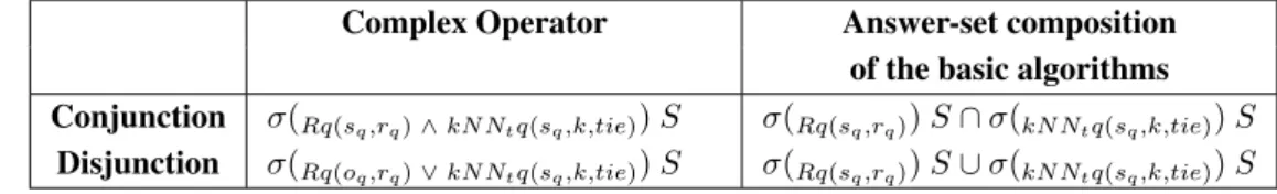
Therefore, it is important to develop algo-rithms that execute often-used complex similarity queries in a much more efficient way instead of the sequential execution of the basic algorithms. This is a required step in extending commercial systems to support complex similarity queries. This work proposes two new algorithms to ex-ecute conjunctions and disjunctions of similarity predicates, two of the most frequently used com-binations of the basic algorithms. Table 2 sum-marizes the correspondence in the execution of the proposed algorithms and the combinations of the basic algorithms to answer queries.
4 Basic Algorithms for Similarity Predicates
This section discusses the basicRange()and
N earest() algorithms which execute the two main types of similarity predicates presented in Section 3.2. The specific case of ties in the
N earest()algorithm is treated in Section 4.1. The range query algorithm Range(sq, rq)
searches the data set S for the elements that are at distancerq from the query centersq or closer.
TheN earest(sq, k)algorithm collects thek
ele-mentssi that are the nearest in data setS to the
query centersq, sorted by the distance from each
element si to the query center. The algorithm
starts computing the distance fromsq to any
ele-ment inS, untilkelements are found, initializing the answer set with those elements. Afterward, a “dynamic radius” keeps track of the largest dis-tance from elementssi tosq. Whenever an
ele-mentsi nearer to sq is found, it replaces the
far-thest one in the answer set, reducing the dynamic radius accordingly.
This description applies both to searching through sequential scan as well as using an in-dexing structure. In the absence of an inin-dexing structure, both algorithms require comparing the query center with every object stored in the data set. Due to the high computational cost to cal-culate the distance between pairs of elements in metric domains, similarity queries commonly use indexing structures to accelerate the processing, since they allow reducing the number of distance calculations by pruning subtrees. Consequently, index structures are even more important in met-ric domains than they are in domains that pos-sess the total ordering property (the typical do-mains of the data handled in current RDBMS). However, sometimes an indexing structure does not exist, as for example when processing the intermediary results from previous selection op-erations, when creating an indexing structure is worthless. Sequential scans can be used in any situation, even when there is no indexing struc-ture, so it is important the algorithms be able to be executed also through sequential scanning.
An index structure recursively groups objects under covering radii centered at representative objects, so the triangular inequality property can prune subtrees using a limiting radius and equations 3 and 4. The limiting radius in the
Range(sq, rq) algorithm is the range radius rq,
thus the pruning ability (“prunability”) of this al-gorithm using index structures is usually high. As there is no static limiting radius to perform ak-nearest neighbor query, the dynamic radius is used as the limiting radius in theN earest(sq, k)
Table 2: Equivalence of the proposed operators and the basic algorithms to answer conjunctive and disjunctive predicates.
Complex Operator Answer-set composition of the basic algorithms Conjunction σ(Rq(sq,rq)∧kN Ntq(sq,k,tie))S σ(Rq(sq,rq))S∩σ(kN Ntq(sq,k,tie))S
Disjunction σ(Rq(oq,rq)∨kN Ntq(sq,k,tie))S σ(Rq(sq,rq))S∪σ(kN Ntq(sq,k,tie))S
4.1 Tie Lists inN earest()Algorithms
The Levenshtein metric LEdit(s1, s2), also
called the edit-string distance LEdit, is a metric
that counts the minimal number of symbols needed to be inserted, deleted, or substituted to transform the string s1 into the string s2. For
example, LEdit( “computer”, “competent”)=3:
two substitutions and one insertion. Searching an English dictionary with 25,153 words for the words differing up to two edit-string operations from the word “computer”has found 7 words: “computer”, “compute”, “copter”, “compacter”, “compote”, “compete” and “commute”, where the
distance from “computer” to the first word is
zero, to the second is one, and to the others is two. If ak-nearest neighbor query withk = 3is posed, that is,
σ(kN N q(“computer”,3))EnglishW ords
then there are five distinct correct answers. How a N earest() algorithm would treat this query? What elements should be returned?
In a first approach, the N earest() algorithm returns justkelements, including the objects that are nearer to the query center than the largest radius found, plus enough objects tied at the largest radius to complete the required quantity
k. This approach returns a non repeatable answer to the query as posing the same query twice can bring different answers. However, it respects the required numberkof elements in the answer. A second approach is to return the answer in two sets: the basic listLb containing the objects that
are nearer to the query center than the largest radius found, and a tie listLt containing all the
objects found at the largest radius distance of
the query center. The answer of this approach is repeatable, but the application receives more than the number k of elements asked. When a tie list is required, the expression governing the
k-nearest neighbor queries must be redefined as:
kNearest Neighbor query with tie list -kN Ntq: given an object sq ∈ S and an integer
value k ≥ 1, thek-nearest neighbor query with tie listσ(kN N
tq(sq,k))S selects at leastk elements
si ∈ S that have the shortest distance from sq
such that:
σ“
kN Ntq(sq,k)
”S=AkN N =Lb∪Lt,
|Lb| ≤k,|Lb∪Lt| ≥k, where
Lb={si|si∈S,
∀sj∈S−Lb⇒d(sq, sj)> d(sq, si)},
Lt={sg, sh|sg, sh∈S, d(sg, sq) =d(sh, sq),
∀si∈Lb⇒d(sq, si)< d(sq, sg),
∀sj∈S− {Lb∪Lt} ⇒d(sq, sj)> d(sq, sg)} (5)
The basic N earest(sq, k) algorithm can be
changed to support answering k-nearest neigh-bor queries with tie lists by including a param-eter tie, which indicates whether tie list should be returned or not. Thus, from now on we use the syntax of the N earest() algorithm as
N earest(sq, k, tie), where tie = true means
that a tie list must be returned in the answer set, otherwise, ties are arbitrarily chosen to returnk
elements.
Thus, rewriting the previous query in this section to
σ(kN Ntq(“computer”,3))EnglishW ords
the answer set for the query is: Lb ∪Lt, where
Lb = { “computer”, “compute”} and Lt = {
We consider that there are two basic ap-proaches that a tie list-enabledN earest() algo-rithm can use to choose elements in theLtlist to
returnkelements when tie-lists are not requested, that we callbiasedandsampledtie lists. Each ap-proach changes the way theN earest()algorithm chooses elements of the internalLt list to return
kelements.
In the biased approach the algorithm proceeds in a deterministic path across the stored data, so that if the database is not updated, two consecu-tive queries asking for the same predicate always return the same answer. As a consequence, some objects that could be part of the answer will never be retrieved, no matter how many times the query is posed. In the sampled tie list, the algorithm in-cludes a random sampling technique to choose the elements of theLt to assure that each query
call will return correct but distinct answers wher-ever more than one exists.
The approach of choice depends on the appli-cation. To many applications, always returning the same answer is an undesirable effect. Com-mon examples are those presenting large tie lists and few updates, such as systems storing health care data, specially those designed for teaching purposes. These databases have most of the at-tributes as categorical ones, leading to large num-ber of ties, and as they store data from selected patients aiming illustration purposes, each one has few updates. Moreover, as the retrieved data is usually employed to feed the human interface modules of the application, the number of neigh-bors asked cannot allow too many samples, so the use of the tie list can be burdensome to the appli-cation and/or the human user. Therefore, present-ing a variety of similar cases at different issues of the same query can be a valuable resource.
To other applications, having the same answer for the same query posed twice is a better op-tion. In this case, the algorithm should prepare the answer in a deterministic way. This occurs for example if whenever an element is found to be inserted at the current tie list, it always replaces
or always not replace those previously chosen to be given as part of the answer set. As both ap-proaches are interesting to different applications, the algorithms presented in the next section em-brace both of them. Therefore, the tie param-eter of the N earest(sq, k, tie) algorithm has its
domain broadened to allow asking for the com-plete tie list (tie = true), a random sample (tie = sample) or a biased subset of the tie list (tie=biased).
Notice that neither approach guarantees a de-terministic kN N q answer, as updates in the database can change the results, even when the update does not change theLb +Ltresult.
Sup-porting a tie list does not increase significantly the computational cost of the N earest() algo-rithm since the number of disk accesses and num-ber of distance calculations remain the same. The total time is only slightly larger in data sets with many ties. We show in Section 6 that this in-crease is indeed almost null.
5 Combining Similarity Operators: The New Algorithms
This section presents the kAndRange() and the kOrRange() algorithms. They follow the branch-and-bound approach and they are de-scribed here considering the data organized fol-lowing a hierarchical MAM with every object stored at the leaf nodes, as the Slim-tree or the M-tree. However, the concept of the algorithms are independent of the particular MAM used and can also be applied on a non indexed data set. We present only the algorithms to search met-ric structures, as their implementation consider-ing sequential scan can be developed straightfor-wardly. As the complex queries involve kN N
predicates, the new algorithms were developed considering the processing of a tie list following the rules expressed as Equation 5.
Eu-clidean metric to generate the figures of this sec-tion, so the radii are represented by circumfer-ences. However, pay attention that, as any metric can be employed, the real shape of the covered areas depends on the metric used.
5.1 Conjunction ofkN N qandRqpredicates
The kAndRange() algorithm performs con-junctive complex similarity query equivalent to aRq(sq, rq)AND akN N q(sq, k, tie) where the
query center is the same. It must recover every object that satisfies both basic similarity predi-cates, that is, the intersection of the intermediate results from both basic operators. Considering a data setS this can be defined as:
σ(R
q(sq,rq))S∩σ(kN N q(sq,k,tie))S ⇔
σ(R
q(sq,rq)∧kN N q(sq,k,tie))S⇔
σ(kAndRq(s
q,rq,k,tie))S
wherekAndRq is the conjunctive predicate exe-cuted by thekAndRange()algorithm.
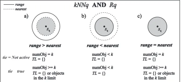
The result of the conjunctive query satisfies the most restrictive condition between the two basic predicates involved, so the condition resulting in the smallest limiting radius contains the final an-swer: the radius of thek-th object of the nearest neighbor operator, which we call the nearest ra-dius, or the query radius of the range operator, which we call the range radius. Figure 1 repre-sents this idea, showing the three possible situa-tions: a) range radius larger than nearest radius; b) range radius shorter than nearest radius; and c) range radius equal to nearest radius.
In Figure 1,sqrepresents the query center, the
continuous-line-border circle shows where the answer to the range predicate can be found, the dashed line border circle shows where the answer to the nearest neighbors predicate can be found, the gray circle is where the answer set of the com-plex query can be found, numObj is the max-imum number of objects recovered by a query,
T L is the tie list and tie states if the tie list is required.
Figure 1.a represents the case when the an-swer is restricted by the nearest-neighbor condi-tion. The answer set in Figure 1.b represents the case when the answer is restricted by the range predicate, and Figure 1.c shows the case when the range radius is equal to the radius of thek-th nearest neighbor, so the answer set contains ev-ery object that satisfies both predicates.
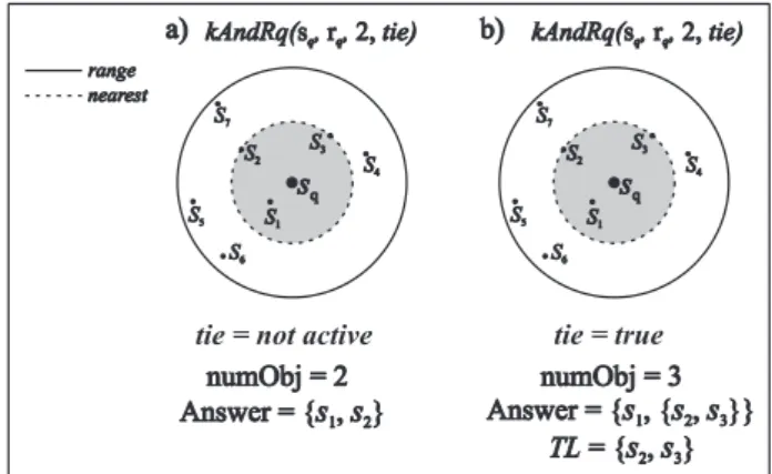
Notice that the number of objects retrieved by a conjunctive similarity query can change de-pending on whether the option tie is active or not, and on whether the answer set is bounded by the nearest-neighbor predicate or not, cases de-picted in both Figure 1.a and 1.c. Figure 2 exem-plify the case when the answer is restricted by the nearest-neighbor condition (case (a) in Figure 1) regarding a data setScontaining seven elements, to answer the predicate kAndRq(sq, rq,2, tie).
Notice that in this case the range condition is looser than the nearest condition, so if the tie list is not required, the number of objects returned
numObj = 2equals the requiredk, as shown in Figure 2.a. If the tie list is required, the number of objects returned can be larger thankto include the whole tie list, as shown in Figure 2.b.
range nearest
numObj = 2 numObj = 2 Answer = { ,s s1 2}
Answer = { ,s s1 2} Answer = { , { ,Answer = { , { ,ss11 s ss s22 33}}}}
TL= { ,s s2 3}
TL= { ,s s2 3} numObj = 3 numObj = 3 tie = not active tie = true a) kAndRq( , ,kAndRq( , ,s r 2,s r 2,qq qq tie)tie) b) kAndRq( , ,kAndRq( , ,s r 2,s r 2,qq qq tie)tie)
sq sq S3 S3
S4 S4 S2
S2
S1 S1 S5 S5
S6 S6 S7 S7
sq sq S3 S3
S4 S4 S2
S2
S1 S1 S5 S5
S6 S6 S7 S7
Figure 2: Tie list in conjunctive similarity queries where the range condition is looser than the near-est condition. a) withtief alse; b) withtietrue.
5.1.1 Algorithms to Manage the tie list
The answer of both thekAndRange()and the
range nearest
numObj =k
numObj =k numObj <numObj <kk numObj =numObj =kk TL= {}
TL= {} TLTL= {}= {} TLTL= {}= {}
numObj >=k
numObj >=k numObj <numObj <kk numObj >=numObj >=kk TL
k
objects in the limit
= {} or
TL k
objects in the limit
= {} or TL
k
objects in the limit
= {} or
TL k
objects in the limit
= {} or
TL= {}
TL= {}
tie = Not active
tie true
range nearest>
range>nearest rangerange<<nearestnearest rangerange==nearestnearest
a) b) c)
sq
sq ssqq ssqq
kNNq
AND
Rq
kNNq
AND
Rq
Figure 1: Graphical representation of the conjunctionkN N∧Rq.
is kept sorted by the distances of each element
si to the query center. This list is managed
by the following methods: Add(obj, distance)
inserts a new element keeping the list sorted;
Length()returns the number of elements in the list; DropLast(k, tie) removes the farthest ele-ment(s) in the list, maintaining the tie list; and
M axDist()returns the largest distance from the query center to an element in the list. The tie list is kept in the end of this list, so the max-imum number of elements stored can be larger than k. Therefore, before return, algorithms
kAndRange()and thekOrRange()must check if a tie list is required and, if not, then the method
ChopAnswer(k) is called to choose a random or a biased subset of elements tied at the farthest distance to be returned.
AlgorithmsAdd(),Length()andM axDist()
are straightforward to be implemented. Algo-rithm DropLast() is shown as Algorithm 1. When called, it drops from the list every ob-ject farther than the obob-ject at position k from the query center. Algorithm ChopAnswer() is shown as Algorithm 2. When tie asks for a bi-ased subset of the tie list, it cuts every object af-ter position k (steps 9 and 10). When tie asks for a sampled subset of the tie list, it randomly remove objects tied with the object at positionk
until onlyk objects remains (steps 2 to 7).
Algorithm 1Answer.DropLast(k, tie)
1: p:=Answer.Length()
2: ifAux > kthen
3: whileAnswer[k].dist < Answer[p].distdo
4: Answer.RemoveLast()
5: p:=p−1
Algorithm 2Answer.ChopAnswer(k)
1: iftie=sample then
2: LargetDist:=Answer[k].dist
3: whileAnswer[k].dist=LargestDist∧k >1do
4: k:=k−1
5: whileAnswer.Length()> kdo
6: p:=Random[LargestDist, Answer.Length()]
7: Answer.Delete(p)
8: else iftie=biased then
9: whileAnswer.Length()> kdo
10: Answer.RemoveLast()
5.1.2 ThekAndRange()Algorithm
The kAndRange(sq, rq, k, tie) algorithm,
shown as Algorithm 3, executes the conjunc-tion Rq(sq, rq) ∧ kN N q(sq, k, tie). It takes
The priority queue contains pointers to the active subtrees, i.e., subtrees where qualifying objects can be found. It has the following two methods: Insert() to add a new active node; and GetN ode() to get the higher priority node. The priority is defined as the distance of the representative of the node srep to the query
center, that isd(srep, sq).
The kAndRange() is a recursive algorithm that receives the root N ode of the (sub-)tree to be traversed, and navigates down to the leaf nodes, applying the triangular inequality prop-erty to prune branches that do not store objects of the answer (see Algorithm 3). This algorithm re-turns the objects that are the nearest to the query center and that are also inside of the range radius. The kAndRange() algorithm starts reading the root node of the (sub-)tree to be traversed (line 1) and, using the priority queueQueue, nav-igates in deep-first mode down to the leaf nodes. It uses the triangular inequality property and the
k and rq limiting values to prune branches that
cannot store objects of the answer. In a non leaf node (lines 14 to 19), this algorithm performs an ordered insertion of subtrees that could not be ex-cluded by the triangle inequality.
Leaf nodes are handled at lines 3 to 13. If an objectsiin a leaf node cannot be pruned based on
the distance between the node representative sp
and the query centersq(Line 5), then the distance
of the objectsito the query center is calculated in
Line 6. If it is inside the range radiusrq (line 7),
si is put in the answer set. Line 6 checks if the
size of the list holding the answer set is shorter than the required numberk of nearest neighbors. If so the objectsiis added to the answer set (Line
8). Otherwise, Line 10 checks if the distance be-tween this object and the query center is smaller or equal to the largest distance between the query center and the objects that are in the result list. When the condition in Line 10 is satisfied, the objectsi is added to the result list, which is kept
sorted by the distances from each object to the query center (Line 11), and theDropLast
func-tion is called (Line 12). This funcfunc-tion uses the numberk of nearest neighbors required and the variable tie to appropriately maintain the result list and the tie list, deleting objects in both if the newly inserted object reduces the current dy-namic radius. Line 13 is an optimization step that reduces the query radiusrq ifk elements nearer
to the query center thanrq were already found.
Algorithm 3 The kAndRange(sq, rq, k, tie)
al-gorithm
1: Queue.Insert(RootN ode,0)
2: while(N ode:=Queue.GetN ode())6=Emptydo
3: ifN odeis a leaf nodethen
4: foreachsi ∈N odedo
5: if|d(sp, sq)−d(si, sp)| ≤rq then
6: Computed(si, sq)
7: ifd(si, sq)≤rqthen
8: ifAnswer.Length()< kthen
9: Answer.Add(si, d(si, sq))
10: else ifd(si, sq) ≤ Answer.M axDist()
then
11: Answer.Add(si, d(si, sq))
12: Answer.DropLast(k, tie)
13: rq:=Answer.M axDist()
14: else
15: foreachsp∈N odedo
16: if|d(sp, sq)−d(srep, sp)| ≤rq+rrepthen
17: Computed(srep, sq)
18: ifd(srep, sq)≤rq+rrepthen
19: Queue.Insert(sq, d(srep, sq))
20: iftie6=true then
21: Answer.ChopAnswer(k)
5.2 Disjunction ofkN N qandRqPredicates
ThekOrRange()algorithm performs disjunc-tive similarity query equivalent to a Rq(sq, rq)
ORakN N q(sq, k, tie)where the query center is
the same. It must recover every object that satis-fies at least one of the complex query predicates, that is, the union of the intermediate results from both basic operators. Considering a data set S
σ(R
q(sq,rq))S∪σ(kN N q(sq,k,tie))S ⇔
σ(R
q(sq,rq)∨kN N q(sq,k,tie))S⇔
σ(kOrRq(s
q,rq,k,tie))S
wherekOrRqis the disjunctive operator.
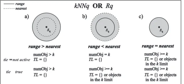
The result of the disjunctive query satisfies any of the two basic predicates involved, so the an-swer consists of the objects covered by the pred-icate with the largest limiting radius. Figure 3 represents this idea, using the same notation of Figure 1. The same three situations described in Section 5.1 occurs with disjunctive queries too.
The answer set shown in Figure 3.a is the range condition. The answer set in Figure 3.b includes every object that satisfies the nearest-neighbor condition, and Figure 3.c shows the case where both the range radius and the radius of the k-th nearest neighbors predicates are equal. The tie list is also considered and it can change the max-imum number of recovered objects as in conjunc-tive queries, which in disjuncconjunc-tive predicates can occur in the case shown in Figure 3.b.
5.2.1 ThekOrRange()Algorithm
The kOrRange(sq, rq, k, tie) algorithm,
shown as Algorithm 4, executes the disjunction
Rq(sq, rq) ∨ kN N q(sq, k). It is similar to the
kAndRange()algorithm, and also uses a global priority queue (Queue) similar to the one used in thekAndRange()algorithm to choose the paths that lead to the best pruning.
ThekOrRange()algorithm starts reading the root node of the (sub-)tree to be traversed (line 1) and, using the priority queue, navigates in deep-first mode down to the leaf nodes. As the range condition cannot define an upper-bound limit for the whole query, the dynamic radius is initially set to infinity in line 2. Whenever a non leaf node is read (lines 14 to 19), this algorithm inserts in
Queuethe subtrees that could not be excluded by the triangle inequality.
Leaf nodes are handled in lines 3 to 16. If an objectsi in a leaf node cannot be pruned based
on the distance between the node representative
sp and the query centersq (Line 6), then the
dis-tance of the object si to the query center is
cal-culated in Line 7. Whenever an object satisfies at least one of the operators, i.e., if object si is
inside the dynamic radiusdk (line 8), it is added
to the answer set (line 9). After the first k ob-jects were already found and a new object is in-serted, the exceeding elements must be deleted from the result (lines 10 to 12). However, this is done only if thedk value is greater than rq,
oth-erwise the object is just inserted, to comply with the disjunction rule. Notice that, the dynamic ra-diusdkis progressively updated as more suitable
elements are found during the search, but it never drops belowrq(lines 13 to 16).
Algorithm 4kOrRange(sq, rq, k, tie) 1: Queue.Insert(RootNode, 0)
2: dk:=∞
3: while(N ode:=Queue.GetN ode())6=emptydo
4: ifNode is a leafthen
5: foreachsi ∈N odedo
6: if|d(sp, sq)−d(si, sp)| ≤dk then
7: Computed(si, sq)
8: ifd(si, sq)≤dkthen
9: Answer.Add(si, d(si, sq))
10: ifdk> rqthen
11: ifAnswer.Length()≥kthen
12: Answer.DropLast(k, tie)
13: if Answer.M axDist()≤rq then
14: dk:=rq
15: else
16: dk:=Answer.M axDist()
17: else
18: foreachsp∈N odedo
19: if|d(sp, sq)−d(srep, sp)| ≤rrep+dkthen
20: Computed(srep, sq)
21: ifd(srep, sq)≤dk+rrepthen
22: Queue.Insert(sq, d(srep, sq))
23: iftie6=true then
range nearest
range>nearest
range>nearest
numObj >k
numObj >k numObj =numObj =kk TL= {}
TL = {} TL TL= {}= {}
numObj >k
numObj >k numObj >=numObj >=kk numObj >=numObj >=kk
numObj >=k
numObj >=k
TL= {}
TL= {} TL
k
objects in the limit
= {} or
TL k
objects in the limit
= {} or
TL k
objects in the limit
= {} or
TL k
objects in the limit
= {} or
TL k
objects in the limit
= {} or
TL k
objects in the limit
= {} or
tie = not active=
tie true
range nearest<
range<nearest rangerange==nearestnearest
a) b) c)
kNNq
OR
Rq
kNNq
OR
Rq
sq
sq ssqq ssqq
Figure 3: Graphical representation of the disjunctionkN N ∨Rq.
5.3 Considerations About the New Algorithms
Prunability. By comparing the two new al-gorithms with the basic alal-gorithms discussed in Section 4, we can do the following considerations related to the query radius. The kAndRange()
algorithm always has a maximum radius defined in the query. Therefore, when the data set is in-dexed by a hierarchical MAM, it prunes subtrees with a high pruning ability (prunability), usually at a much higher rate than the one obtained by the basic nearest neighbor algorithm. This is due to the basic k-nearest neighgbor algorithm can-not use a limiting radius initially. In the exper-iments we verified that the kAndRange() algo-rithm always has a prunability and a performance equivalent or better than those of the basic range query algorithm, which in turn usually have a much higher prunability then the basicN earest
algorithm.
The kOrRange() algorithm does not have a maximum radius defined in the query parame-ters, and presents a lower prunability than the
kAndRange() algorithm. However, as it also evaluates two predicates at once, it has a prun-ability higher than the prunprun-ability of the basick -nearest neighbor algorithm.
Algebraic Rules. To define algebraic rules to guide optimization processes of complex queries
is not the objective of this paper. However, the proposed algorithms were designed considering that algebraic rules could be applied. There-fore, we show here four algebraic rules that give an intuition of how these rules can be used by the query optimizer enabling the proposed algo-rithms to answer complex similarity queries. In fact, a complex similarity query involving two basic similarity predicates of the same type (that is, two Rq or two kN N q predicates) with the same central object can be changed into one basic query of the same type. This can be performed by suitably choosing the respective radius or number of objects, observing the following rules for con-junctive or discon-junctive similarity queries:
AND:
1. σ(Rq(sq,rq1))S ∧ σ(Rq(sq,rq2))S|rq1≤rq2 ⇐⇒σ(Rq(sq,rq1))S 2. σ(kN N q(sq,k1,tie))S ∧ σ(kN N q(sq,k2,tie))S | k1≤k2 ⇐⇒ σ(kN N q(sq,k1,tie))S
OR:
1. σ(Rq(sq,rq1))S ∨ σ(Rq(sq,rq2))S | rq1≤rq2 ⇐⇒ σ(Rq(sq,rq2))S
Using these rules, a query optimizer can change any expression involving multiple simi-larity predicates centered at the same query cen-ter into an expression that can be answered by the two proposed algorithms.
Multiple Centers. The composition consid-ering more than one similarity predicate of the same type (RqorkN N q) with distinct query ob-jects can also be changed into only one query of the same type. This can be performed by a suit-able choice from respective radius or object num-bers, applying the algorithms proposed in this pa-per, and filtering their results. For example, two range queries can be executed by choosing one of them as the complex query center, and setting the query radius as the summation of their basic radii extended by the distance between the centers of the complex similarity query. After executing the changed query, the results are compared to each one of the original centers, thus filtering the fi-nal answer. The calculation of the corresponding query radius or object numbers to be used in the algorithms proposed in this paper and the filter-ing of their results can be executed usfilter-ing alge-braic rules. This allows using the proposed algo-rithms to answer any complex similarity query.
6 Experiments
This section presents experimental measure-ments on the proposed algorithms, comparing them with the correspondent measurements ob-tained by compositions of the basic algorithms. Every algorithm was implemented in two ver-sions: through a sequential scanning over the data set (SeqScan) and using the Slim-tree met-ric access method. The algorithms were im-plemented in C++, and the experiments were run in an Intel Pentium-4 1.6GHz machine, with 512MB of RAM memory and a 40GB disk spin-ning at 7200RPM, under the Microsoft Windows 2000 operating system. The following subsec-tion presents the settings that we have used in experiments and Subsection 6.2 shows the
mea-surements obtained.
6.1 Experimental Setup
To evaluate the performance and efficiency of the proposed algorithms, we have used a vari-ety of data sets, both synthetic and from the real world, although in this paper we present only the results obtained from the following four data sets.
• Synthetic- a synthetic set of points uni-formly distributed in 6-dimensions;
• LBeach - a set of geographical points in a 2-dimensional space describing the coordinates of the road intersections in Long Beach City, CA, from the TIGER system of the U.S. Bureau of Census;
• CorelHisto - a set of attributes de-scribing colors in images in 32 di-mensions, from the UCI repository (kdd.ics.uci.edu);
• Words- a set of words extracted from a Portuguese language dictionary [20]. For theWordsdata set we used the Levenshtein metric. The other are dimensional data sets, so we used the Euclidean metric (L2). The object
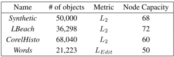
size changes in each data set, so the maximum node capacity of the Slim-tree changes too, to test trees using the same node size of 4kBytes. The properties of the four data sets and the maximum node capacity are summarized in Table 3.
Table 3: Data sets used in the experiments.
Name # of objects Metric Node Capacity
Synthetic 50,000 L2 68
LBeach 36,298 L2 72
CorelHisto 68,040 L2 60
Words 21,223 LEdit 50
N earest() algorithm, the Range() algorithm and then the set union or the set intersection oper-ator. The set operators are performed in memory. Every measurement represents the average of 500 queries regarding the number of distance cal-culations, the number of disk accesses and the to-tal time in milliseconds. Each set of 500 queries has its query center object chosen in the follow-ing way: 250 were sampled from the respec-tive data set but were kept in the data set; the other 250 objects were sampled from the respec-tive data set and removed from it. Therefore, the queries cover both the biased queries regarding the distribution of the data set elements and the randomly distributed queries scattered in the data domains, both of them occurring in real applica-tions. Each measurement considers a range ra-dius rq and a fixed number k of nearest
neigh-bors, averaging the results over the set of 500 query centers. In each plot, the abscissa repre-sents the number of objects retrieved, expressed as a percentile of the data set.
In each experiment, the number of neighbors and the range radius varies as follows. The ra-dius for the Synthetic, LBeach and CorelHisto data sets varies from 0.01% up to 10% of the data set diameter. For the Words data set the radius varies from 1 up to 10 editions. The values ofk
for the Synthetic, LBeach and CorelHisto is re-spectively 0.01%, 0.02%, 0.05% of the data set, and is 5 words for theWordsdata set.
6.2 Performance Evaluation
This section presents the results obtained from the kAndRange(), kOrRange() and the ba-sic algorithms both searching a Slim-tree and through the SeqScan.
Figure 4 compares the proposed and the basic algorithms to answer 500 queries in the four data sets. The plots are presented in log-log scale for theSynthetic, LBeach, CorelHisto data sets, and in linear-log scale for theWordsdata set. Every experiment asks for the tie list. The figure shows
the plots of the average number of disk accesses (Figures 4.A, D, G and J), the average number of distance calculations (Figures 4.B, E, H and K), and the total time (Figures 4.C, F, I and L).
Considering the SeqScan, the union/intersec-tion of the basic algorithms (plots F and H in the graphs) and kOrRange()/kAndRange() al-gorithms (plots E and G) present a constant num-ber of disk accesses and distance calculations considering query range and k. However, the traditional approach requires twice as many dis-tance calculations and number of disk accesses as our proposed algorithms. Searching the Slim-tree using either the union or intersection of ba-sic algorithms (plots B and D) has the same number of disk accesses and of distance calcu-lations. However, either the kAndRange() or
kOrRange()algorithms (plots A and C) requires up to 30% less disk acesses and distance calcu-lations. Moreover, the kandRange() algorithm grow linearly up to the maximum variation of
k and then assumes a sub-linear behavior, and tends to stabilize (plot A). This is easily seen in theCorelHistodata set, as shown in Figures 4.G and 4.H.
The new algorithms have a different behavior when using the Slim-tree in the Words data set (Figures 4.J and 4.L), as both algorithms have closer behavior and their numbers of disk ac-cesses and distance calculations quickly become constant. This happens because the results of the LEditdistance function give discrete values
and produces many ties. Figure 4.J shows that the Slim-tree requires a number of disk accesses larger than the SeqScan. This is because the Slim-tree requires more disk space to store the structure itself. However, as the number of dis-tance calculations drops as shown in 4.L, the to-tal time of every algorithm is smaller in the Slim-tree than in its SeqScan counterpart (4.M).
to-Figure 4: Comparing the performance to answer 500 queries using the proposed and the basic algorithms using the Slim-tree and the SeqScan, on theSynthetic, LBeach, CorelHistoandWordsdata sets. (A, D, G, J) Average number of disk accesses per query. (B, E, H, K) Average number of distance calculations per query. (C, F, I, L) Total time for 500 queries in seconds.
tal time grows too, as is evidenced in the algo-rithms searching a Slim-tree. Besides, it must be noticed that the union/intersection operations just affect the time measurements of the SeqS-can accesses (plots E, F, G and H). When
the Synthetic data set. The kOrRange() Algo-rithm is about two times faster than the union of the basic algorithms for small radii, increasing to be up to 3 times faster for large values of radii, as shown in Figure 4.F for theLBeachdata set.
Regarding the Slim-tree, the new algorithms provide higher improvements in every measured aspect. ThekAndRange()algorithm requires at most half the numbers of distance calculations, of disk accesses and total time to process queries with small radii in every data set tested, as com-paring with the intersection of the basic algo-rithms (plots A and B). For higher values of radii, e.g., when retrieving 10% of the data set, the re-duction is even larger: it reduces to1/12of the number of disk accesses in the LBeach data set (Figure 4.D), to1/23of the number of distance calculations in Synthetic data set (Figure 4.B), and to less than one hundredth of the total time in the LBeach and Synthetic data sets (Figures 4.C and 4.F). The kOrRange() algorithm also requires equivalent reduction compared to the union of the basic algorithms for small radii in al-most all data sets (plots C and D). The exception happens to the Words data set, where for small radii the reduction is larger, as thekOrRange()
algorithm reduces to almost 50% every measured aspect (Figures 4.J, 4.L and 4.M). For small val-ues of radii (less than 0,2% of the data set, the gain of thekOrRange()algorithm decreases to only 10% in the number of disk accesses and dis-tance calculations in LBeach and Random data sets (Figures 4.A, 4.B, 4.D and 4.E). However, theWordsdata set is again an exception, once this new algorithm achieved improvements of at least twice in every measured aspect as compared with the union of the basic algorithms.
It is interesting to note that the proposed al-gorithms provide the most remarkable improve-ments in the total time for the queries most fre-quently used in real systems, i.e., those queries with small range radius and few neighbors. Moreover, the experiments show that every mea-surement performed using thekAndRange()or
kOrRange() algorithms presented better per-formance than the correspondent intersection or union of the basic algorithms, either searching a Slim-tree or using a SeqScan.
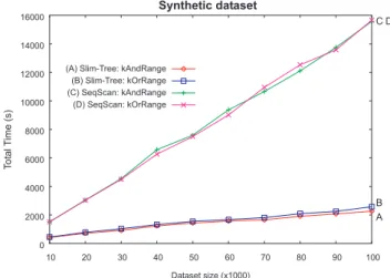
In another experiment using theSyntheticdata set, we generated the data set in 10 steps, adding 10,000 elements at each step, and for each database size we measured the total time to cal-culate 500 queries usingk = 0,1%of the number of elements in the database andr1 = 0,1%of the
data set diameter. The result, shown in Figure 5, shows that the proposed algorithms present lin-ear behavior when varying the data set size, so they are scalable regarding the data set size. It also shows that as the data set size increases, the more important is the use of a MAM.
(A) Slim-Tree: kAndRange (B) Slim-Tree: kOrRange (C) SeqScan: kAndRange (D) SeqScan: kOrRange
0 2000 4000 6000 8000 10000 12000 14000 16000
10 20 30 40 50 60 70 80 90 100 Dataset size (x1000)
Synthetic dataset
T
ot
al
T
ime(s)
A B C D
Figure 5: Measurement of wall-clock time to ex-ecute 500 queries using the kAndRange() and thekOrRange()algorithms using both SeqScan and Slim-tree with varying data set size, showing the scalability of the algorithms.
6.2.1 Measurements involving the tie list
kOrRange() algorithm. This is due to the fact that both algorithms prune subtrees that are far-ther than the region covering the algorithm’s lim-iting radius, but does not exclude nodes that are at nearer or at equal distance as the limiting ra-dius. Thus, when an object in a leaf node qual-ifies, it is added in the answer set and only then the Answer.DropLast() method can check the
tievariable to determine if the new object will be maintained in the answer set or not. Therefore, the numbers of disk accesses and of distance cal-culations are not affected, which was confirmed in the experimental measurements.
However, the total time can change when a tie list is required. This happens because managing the answer set is slightly more complex when the tie list is required. The experiments show that total time increases proportionally to the number of ties, but very slowly. Although we evaluated every data set presented in this paper, only the Worddata set presented measurable differences.
Figure 6 shows the total time in conjunctive and disjunctive queries measured in the Words data set, comparing when asking for a biased tie list, for a sampled tie list or for no tie list. BothkAndRange()andkOrRange() algo-rithms were tested searching a Slim-tree, because being it faster, processing the tie list have a larger impact in the total time. Notice that the increase in total time is so slightly that it is barely visi-ble in Figure 6. Numerically, thekAndRange()
algorithm takes 59.92s to calculate 500 queries withk = 3andrq = 9without a tie list. The total
time increases 0.063s when asking for a biased tie list, and 0.344s when asking for a sampled tie list. ThekOrRange()algorithm takes 2055.95s to calculate 500 queries with k = 3 and rq = 9
without a tie list, increasing 0.078s when asking for a biased tie list, and 6.640s when asking for a sampled tie list.
10 100 1000 10000
1 2 3 4 5 6 7 8 9 10
Radii
Words: k<3
(C) Slim-tree kAndRange TIE=Sample (A) Slim-tree kAndRange TIE=Biased (B) Slim-tree kAndRange TIE=True
(D) Slim-tree kOrRange TIE=Biased (E) Slim-tree kOrRange TIE=True (F) Slim-tree kOrRange TIE=Sample
T
ot
al
T
ime(s)
A D
B E
C F
Figure 6: Comparing total time to answer 500 queries using kAndRange() and kOrRange()
algorithms over the Slim-tree, with and without the tie list.
7 Conclusions
This paper presented two new algorithms, called kAndRange() and kOrRange(), that were developed to support the composition of simi-larity operators using conjunction and disjunc-tion between range andk-nearest neighbor con-ditions in complex similarity queries centered at the same query object. These algorithms were created aiming to support a tie list in the result. A tie list enables to control two problems exist-ing in algorithms that involves the kNNq oper-ator: the non repeatability answering similarity queries and the hiding of results that can be rele-vant in queries, as discussed in Section 4.1.
algo-rithms reduce the total time and numbers of disk accesses and distance calculations to at most half, improving the most frequent queries posed in real systems. Moreover, the experiments showed that the new algorithms reduced up to 12 times the number of disk accesses, more than 20 times the number of distance calculations and can be more than a hundred times faster than the correspon-dent composition of the basic algorithms.
Notice that to answer those queries without the new algorithms it is necessary to run the ba-sic algorithms individually, composing the inter-mediate results through intersections or unions to produce the final result. Therefore, the main contribution of this paper is enabling RDBMS to perform complex similarity queries in a prac-tical way, through the inclusion of the similar-ity operators as an extension of SQL. In addi-tion, this paper makes it possible to develop de-sirable characteristics in similarity queries as fu-ture works, such as the support for a query opti-mizer to handle similarity queries through a set of algebraic rules covering similarity predicates, changing of any expression involving multiple similarity predicates centered at the same query center into an expression that can be answered by the two proposed algorithms, or developing the support for the composition of similarity queries with distinct centers, as briefly suggested in Sec-tion 5.3.
References
[1] 13249-3:2001, I. (2001). Information tech-nology – Database Languages – SQL Multi-media and Application Packages – part 3: Spa-tial – ISO/IEC.
[2] Arantes, A. S., Vieira, M. R., Traina Jr., C., and Traina, A. J. M. (2003). Operadores de se-leção por similaridade em sistemas de gerenci-amento de bases de dados relacionais. InProc. of the XVIII SBBD, pages 341–355, Manaus, Brasil.
[3] Araujo, M. R. B., Traina, A. J. M., and Traina, Caetano, J. (2002). Extending SQL to support image content-based retrieval. In Proc. of IASTED ISDB, page 6, Tokyo, Japan. [4] Benetis, R., Jensen, C. S., Karciauskas, G., and Saltenis, S. (2002). Nearest neighbor and reverse nearest neighbor queries for moving objects. In Nascimento, M. A., Özsu, M. T., and Zaiane, O. R., editors,Proc. of IDEAS’02, pages 44–53, Edmonton, Canada. IEEE Com-puter Society.
[5] Berchtold, S., Ertl, B., Keim, D. A., Kriegel, H.-P., and Seidl, T. (1998). Fast nearest neigh-bor search in high-dimensional space. InProc. of the 14th ICDE, pages 209–218, Orlando, USA. IEEE Computer Society.
[6] Böhm, K., Mlivoncic, M., Schek, H.-J., and Weber, R. (2001). Fast evaluation techniques for complex similarity queries. In Apers, P. M. G., Atzeni, P., Ceri, S., Paraboschi, S., Ra-mamohanarao, K., and Snodgrass, R. T., edi-tors, Proc. of the 27th VLDB, pages 211–220, Roma, Italy. Morgan Kaufmann.
[7] Chaudhuri, S. and Gravano, L. (1996). Op-timizing queries over multimedia repositories. InProc. of SIGMOD, pages 91–102, Quebec, Canada.
[8] Cheung, K. L. and Fu, A. W.-C. (1998). En-hanced nearest neighbour search on the R-tree. ACM SIGMOD Records, 27(3):16–21.
[9] Chávez, E., Navarro, G., Baeza-Yates, R., and Marroquín, J. L. (2001). Searching in met-ric spaces. ACM Computing Surveys (CSUR), 33(3):273–321.
[10] Ciaccia, P., Patella, M., and Zezula, P. (1997). M-tree: An efficient access method for similarity search in metric spaces. In Jarke, M., editor,Proc. of the 23th VLD), pages 426– 435, Athens, Greece. Morgan Kaufmann Pub-lishers.
(1998). Processing complex similarity queries with distance-based access methods. InProc. of EDBT, volume 1377, pages 9–23, Valencia, Spain.
[12] Fagin, R. (1996). Combining fuzzy infor-mation from multiple systems. In Proc. of ACM SIGMOD-PODS, pages 216–226, Mon-treal, Canada.
[13] Faloutsos, C. (1997). Indexing of multime-dia data. InMultimedia Databases in Perspec-tive, pages 219–245. Springer Verlag.
[14] Guttman, A. (1984). R-tree: A dynamic index structure for spatial searching. In Yor-mack, B., editor, Proc. of the 1984 ACM-SIGMOD, pages 47–57, Boston, USA. ACM Press.
[15] Hibino, S. and Rundensteiner, E. A. (1998). Processing incremental multidimen-sional range queries in a direct manipulation visual query. InProc. of the 14th IEEE-ICDE, pages 458–465, Orlando, USA. IEEE Com-puter Society.
[16] Hjaltason, G. R. and Samet, H. (1999). Dis-tance browsing in spatial databases. ACM Transactions on Database Systems (TODS), 24(2):265–318.
[17] Katayama, N. and Satoh, S. (1997). The SR-tree: An index structure for high-dimensional nearest neighbor queries. In Peckham, J., editor, Proc. of the 1997 ACM-SIGMOD, pages 369–380, Tucson, USA. ACM Press.
[18] Korn, F., Sidiropoulos, N., Faloutsos, C., Siegel, E., and Protopapas, Z. (1996). Fast nearest neighbor search in medical image databases. In Vijayaraman, T. M., Buch-mann, A. P., Mohan, C., and Sarda, N. L., ed-itors,Proc. of the 22th VLDB, pages 215–226, Mumbai (Bombay), India. Morgan Kaufmann. [19] Melton, J. and Eisenberg, A. (2001). SQL multimedia and application packages
(SQL/MM). ACM SIGMOD Records, 30(4):97–102.
[20] Nunes, M. G. V., Vieira, F. M. C., Zavaglia, C., Sossolote, C. R. C., and Hernandez, J. (1996). A construção de um léxico da Língua Portuguesa do Brasil para suporte à correção automática de textos. Relatórios técnicos do ICMC, USP - São Carlos - SP.
[21] Park, D.-J. and Kim, H.-J. (2003). An enhanced technique for k-nearest neighbor queries with non-spatial selection predicates. Multimedia Tools and Applic., 19(1):79–103. [22] Roussopoulos, N., Kelley, S., and Vincent,
F. (1995). Nearest neighbor queries. In Carey, M. J. and Schneider, D. A., editors, Proc. of the 1995 ACM SIGMOD, pages 71–79, San Jose, USA. ACM Press.
[23] Traina, Caetano, J., Traina, A. J. M., Falout-sos, C., and Seeger, B. (2002). Fast index-ing and visualization of metric datasets usindex-ing Slim-trees. IEEE Transactions on Knowledge and Data Engineering (TKDE), 14(2):244– 260.
[24] Traina, Caetano, J., Traina, A. J. M., Seeger, B., and Faloutsos, C. (2000). Slim-trees: High performance metric trees minimizing overlap between nodes. In Zaniolo, C., Lockemann, P. C., Scholl, M. H., and Grust, T., editors, Proc. of EDBT’2000, volume 1777 ofLNCS, pages 51–65, Konstanz, Germany. Springer. [25] White, D. A. and Jain, R. (1996). Similarity