Todos os direitos reservados.
É proibida a reprodução parcial ou integral do conteúdo
deste documento por qualquer meio de distribuição, digital ou
impresso, sem a expressa autorização do
Child Labor and Learning
Patrick M. Emerson
Vladimir Ponczek
André Portela Souza
CHILD LABOR AND LEARNING
Patrick M. Emerson
Vladimir Ponczek
André Portela Souza
Patrick M. Emerson Department of Economics Oregon State University 313 Ballard Hall
Corvallis, Oregon 97331
Vladimir Ponczek
Escola de Economia de São Paulo Fundação Getúlio Vargas (EESP/FGV) Rua Itapeva, nº 474, 12º andar
01332-000 - São Paulo, SP - Brasil
André Portela Souza
Escola de Economia de São Paulo Fundação Getúlio Vargas (EESP/FGV) Rua Itapeva, nº 474, 12º andar
Child Labor and Learning
∗
Patrick M. Emerson
†Vladimir Ponczek
‡Andr´
e Portela Souza
§August 16, 2013
Abstract
This paper investigates the impact of working while in school on learning outcomes
through the use of a unique micro panel dataset of students in the S˜ao Paulo municipal
school system. The potential endogeneity of working decisions and learning outcomes
is addressed through the use of a difference-in-difference estimator and it is shown
that the results are robust. A negative and significant effect of working on learning
outcomes in both math and Portuguese is found. The effects of child work from the
benchmark regressions range from 3% to 8% of a standard deviation decline in test
score which represents a loss of about a quarter to a half of a year of learning on
average. Additionally, it is found that this effect is likely due to the interference of
work with the time kids can devote to school and school work.
JEL classification: J13,I21.
Keywords: Child Labor; Learning; Proficiency; Education.
∗Acknowledgements: For useful comments and advice, we thank seminar participants at the S˜ao Paulo School of Economics. For outstanding research assistance we thank Eduardo Tillman. We thank the Funda¸c˜ao de Amparo `a Pesquisa do Estado de S˜ao Paulo (FAPESP) for financial support.
†Corresponding Author: Oregon State University, IZA & C-Micro, S˜ao Paulo School of Economics, FGV
1
Introduction
Though the global trend is downward, the incidence of child labor remains very high in
developing countries. For example, in 2000 the International Labour Organization estimated
that 246 million, or almost 16 percent, of the world’s children between the ages of 5 and
17 were child laborers. By 2008 this had fallen to 215 million - a dramatic decline but
still representative of 13.6 percent of the world’s children. In response, many governments
have proposed or implemented policies designed to reduce the incidence either in their own
countries, through labor laws that restrict or prohibit children working, or in other countries,
through policies such as restricting the importation of goods that use children in some part
of their production.
However, much of this policy discussion has taken place in an information scarce
envi-ronment. While much is known about the incidence and the determinants of child labor,
surprisingly little is known about the consequences of child work on participants. Important
policy questions such as how young is too young to work, are some work activities better or
worse than others, does work impair the health of children and does combining work and
school hinder learning remain largely unanswered. This paper seeks to provide an answer
the last of these questions and contributes to the literature by assessing the impact of
work-ing while in school on learnwork-ing as measured by the proficiency of students in the S˜ao Paulo
municipal school system through their performance on standardized exams.
Perhaps the main reason for the dearth of received evidence on the impact of child work
is the inherent difficulty in uncovering causal linkages between the activities of children
and their subsequent outcomes. The effects of confounding and unobserved variables are
persistent problems that are difficult to overcome. In this study, we utilize a unique panel
that allow us to explore the causal link between the work activity of children and its effect
on their exam performance.
We find that, controlling for individual time-invariant unobservable characteristics,
work-ing while remainwork-ing in school has a depresswork-ing effect on their proficiency test scores. The
magnitude of these effects range from 3% of a standard deviation in test scores to 8% which
represents from one quarter to one half of a year of lost learning. The results are robust
to idiosyncratic preferences and we perform robustness checks to show that the results are
not due to idiosyncratic trends or economic shocks at the household level. Additionally, we
find that the magnitude of the negative impact increases with a students ability and that
there are both lingering and cumulative negative effects from working whir in school. These
results provide valuable information to policy makers who wish to understand what types of
child work to target for elimination and the effect of child labor on human capital
accumu-lation. Finally, we find possible channels through which child labor can impact learning as
participants in the labor market are more likely to report that they miss school days, turn
homework in late and complete homework while in school rather than at home.
In recent years, a large body of theoretical and empirical research has emerged that has
studied the economics of child labor (see Edmonds, 2008; Edmonds and Pavcnik, 2005; Basu
and Tzannatos, 2003; Basu, 1999, for extensive literature reviews). Much of the received
empirical work has focused on the determinants of child labor while questions of the
con-sequences of child labor have been largely contained in the theoretical literature (see e.g.
Edmonds, 2008; Edmonds and Pavcnik, 2005; Basu and Tzannatos, 2003; Basu, 1999;
Emer-son and Knabb, 2007, 2006, 2008; Horowitz and Wang, 2004; Ejrnæs and P¨ortner, 2004;
Basu, 2002; Dessy and Pallage, 2001; Baland and Robinson, 2000; Dessy, 2000; Basu and
and human capital accumulation to justify policy interventions assuming depressing impacts
from child labor. As noted above, the empirical foundations to support these assumptions
are weak. 1
Though evidence of the effects of child work on participants is still relatively scarce,
there is a new and growing literature that has begun to fill in the lacuna. Beegle et al.
(2009), studies a five year panel of school children in Vietnam and finds that child labor
has negative consequences on school participation and educational attainment. Orazem and
Lee (2007) uses Brazilian household data to examine the impact of working as children on
self-reported health outcomes and finds negative impacts of child labor. Emerson and Souza
(2011) examines retrospective data from Brazil and finds that child work before 13-14 years
old negatively affects adult incomes, but that this affect turns positive after these ages.
Interestingly, this study finds that the effect of child work on earnings remain even when
controls for years of education are included, raising the possibility that child labor may
affect the learning of those workers who remain in school, which provides a motivation for
the current study.
Research on the consequences of child work on education have mainly focused on
atten-dance rather than learning (e.g. Ravallion and Wodon, 2000; Assaad et al., 2001;
Canals-Cerda and Ridao-Cano, 2004; Beegle et al., 2008, 2006; Assaad et al., 2005) and have found
modest negative effects of child work. But as Emerson and Souza (2011) suggest, school
enrollment may not be the only important measure, especially in countries like Brazil where
combining work and school are common.
The direction of the expected impact of child work on learning is unclear. Working
requires time and energy that could hamper a student’s ability to learn, but some work
1
activities could involve tasks that are either directly related to learning (like reading, writing
and math) or indirectly related but still involve use of these skills. If a work activity involves
learning-by-doing or is otherwise positively correlated to learning the skills tested in school
(in our case math and Portuguese), work could, in fact, have a positive impact. In the end
the true nature of the relationship between work and learning, if the two are substitutes or
complements, is an empirical issue.2 Understanding this relationship is extremely important
as previous research has shown a very strong connection between educational proficiency
and adult income and economic growth, and that proficiency is a stronger determinant than
completed years of schooling [see, e.g. Hanushek and Zhang (2009) and Hanushek and Kimko
(2000)].
We are aware of three previous studies that have examined the impact of child work
on student proficiency. The first paper, closely related to the present study is Bezerra et
al. (2009), which uses cross-sectional Brazilian data to test the impact of working on the
performance on similar exams. The authors find that working has a negative impact on the
performance of participants. Another closely related study is Dumas (2012) which exploits
retrospective data from Senegal to examine the effects of child work on the test scores
of Senegalese children and finds some evidence of positive effects of child work. Finally
Gunnarsson et al. (2006) uses data from nine Latin American countries (including Brazil) and
finds negative and significant impacts of working on student test scores. All three studies are
constrained by the inherent difficulties in overcoming the potential endogeneity of child labor
and both implement instrumental variables strategies in an attempt to overcome the problem.
In all three cases, the challenge of finding sources of variation that are correlated with the
decision to work but uncorrelated with the unexplained variation in school performance is
2
severe, leading to questions of the validity of the instruments themselves and thus the results.
In our case the use of time-series data presents a huge advantage in our ability to control for
both the endogeneity of child labor and the presence of other unobservables (e.g. parental
preferences) that are potentially correlated with both the decision to work and the aptitude
for, and attitude toward, school. We are also able to explore the lingering and cumulative
impacts of child labor as well as explore the heterogeneous effects on student of different
ages and abilities. In addition, through the time-use information available to us, we are able
to explore the potential channels through which child labor may interact with the process of
learning and we are thus able to shed light on the mechanisms involved.3
This paper proceeds as follows: In section 2 we describe the data used in the study. In
section 3 we describe the general child labor and educational environment in the City of S˜ao
Paulo. In section 4 we explain the empirical strategy, how we identify our model and the
robustness checks we employ. In section 5 we present and discuss the results of the empirical
investigation. In section 6 we summarize the paper and discuss the policy implications of
the results of the empirical investigation.
2
Data, Sample Selection and Descriptive Statistics
In 2007, the City of S˜ao Paulo started an evaluation system for students enrolled in municipal
schools involving a set of proficiency exams in mathematics and Portuguese. These exams
were accompanied by a questionnaire that was given to each student taking the exams as well
as an additional questionnaire that was given to the parents of the students taking the exams
about the socio-economic characteristics of the family, although the parents questionnaire
3
was not administered in 2008.4 The exam is called the Prova S˜ao Paulo (S˜ao Paulo Exam)
and was implemented annually until 2013 when it was discontinued. The microdata from
the 2007 to 2010 exams are available and used in this paper. In 2007 all students in the
even grades (2nd,4th,6th and 8th) took the exam. In 2008, all students in the 2nd,4th and 6th
grades took the exam, and randomly selected students in 3rd,5th, 7th and 8th grades took the
exam (one class per grade per school was randomly selected to take the exam). From 2009
and on, all students in the even grades and randomly selected students in the odd grades
(35 students per grade per school) took the exam.5 In each year, around 500,000 students in
8,000 classes in 500 schools took the exam. Importantly, the S˜ao Paulo Exam was structured
based on the Item Response Theory (IRT) so that the results are comparable across grades
and across years.
We have information from the students’ questionnaires for all years on the students’
working status. Only students in the fifth grade and above answer the question about child
labor, which restricts the population of analysis.6 The precise wording of the question about
working status is as follows (translation ours):
“During school days, do you work?
(A) Yes, outside of the house; (B) Yes, at home helping with the chores; (C) No, I only
study.”
Respondents were limited to one answer only. We set the indicator variableM arketLabor
equal to 1 whenever a student answered ”A”, and to 0 otherwise so we are comparing those
4
Questionnaires were also given to the principals which asked them to answer questions about themselves, their school, the teachers and supervisors, and the student population, but it was not administered in 2009.
5
All students in the fifth grade who scored below 150 points in the previous year are also included in sample.
6
that work outside of the home to those who work at home on chores and those who do not
work at all.
From the parent’s questionnaire we collected information about the father’s employment
status for 2007, 2009 and 2010.
The student questionnaire also asks students about their studying habits such as whether
they miss classes, hand in homework late, prepare for exams in advance, and complete
home-work at school. From the responses to these questions we created four indicator variables.
We construct three different samples for this study. The first includes all observations of
students in the 6th,7th and 8th grades in 2007, 2008, 2009 and 2010. This sample constitutes
an unbalanced panel of 473,051 observations of 313,297 students (158,180 boys and 155,117
girls).7 We call this the “full sample”. The second sample encompasses all students that
were in 6th grade in 2007 or in 2008 and were found two years later from the first observation.
Therefore, we have exactly two observations for each student. This balanced panel has 48,009
boys and 48,161 girls. We call this the “paired sample”. The third sample also encompasses
all that were in 6thgrade in 2007 or in 2008, but we include only those who were also found in
next two consecutive years after the first observation. Depending on the exercise, we use the
first and third observations or the first and second observation for each students. Therefore,
we have exactly two observations for each student. The sample contains observations on
6,563 boys and 6,630 girls and we call this the “3 period sample.”8
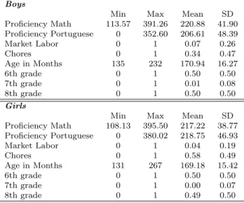
Tables 1 to 3 presents some descriptive statistics of the three samples separately for boys
and girls. The incidence of child labor in the full sample is around 12% for boys and 6% for
7
We also dropped 994 students aged nine years old or below. We believe those are measurement error, since the regular age for the 6th
grade in Brazil is 12 years old. Nevertheless, none of the deleted students appear more than once in the sample, therefore the trimming does not change the estimate of the parameter of interest in the fixed effect specification.
8
girls. The average age is 14 years old and, on average, boys outperform girls in math and
the reverse occurs in Portuguese.
[INSERT TABLES 1 AND 2 AND 3 AROUND HERE ]
Since we use fixed effect estimators, it is necessary for identification to have transitions
into and out of market labor. Table 4 shows the transition matrix of the market labor
variable. We can see that for both boys and girls we have a sufficient number of students
transiting in and out of working status. For instance, 4,500 boys and 2,300 girls change their
status from not working to working in one year.
[INSERT TABLE 4 AROUND HERE ]
It is worth noting here that we observe only those who are enrolled in the S˜ao Paulo
municipal school system and who remain in the school system. There is no forced repetition
of grades in S˜ao Paulo municipal schools for the 6th,7th and 8th grades, but there can be
drop-out, movement to state or private schools or movement out of the area. As drop-out
and delay are likely two other important effects of child labor, it is important to note that
we are not examining these ancillary effects of child labor.
3
Child Labor and Students in the City of S˜
ao Paulo
This section describes the incidence of child labor and school attendance in the City of S˜ao
Paulo.9 The data used in this study come from the 2010 Demographic Census collected by
the Brazilian Census Bureau (IBGE). It contains information on socio-demographic
charac-teristics, fertility, migration, and time allocation for all individuals sampled. It is a sample
of the entire population representative at the municipality level. Most important for the
9
present study, it contains information about school attendance, labor force participation
and occupation in the reference month of the survey (July). The information for labor
market outcomes are available for individuals aged 10 years old and above.
3.1
Child Laborers
Table 5 below presents the figures for the time allocation of individuals aged 10 to 17 living
in S˜ao Paulo City in 2010 for male and female individuals, separately. There are around 1.4
million individuals in this category and the majority attend school. In fact, 85.4% (86.6%) of
boys (girls) attend school only; and 6.2% (5.4%) of the boys (girls) divide their time between
school and work. Thus around 92% (93%) of boys (girls) attend school. Conversely, 2.5%
(1.7%) of boys (girls) work only; and 5.9% (6.3%) of boys (girls) neither work in the labor
market nor attend school. Summing up those that work only and those that work and attend
school, the incidence of child and adolescent work among boys is 8.7% and among girls it
is 7%. Note that of all boys working in the labor market, 71% attend school, and for girls
the figure is 76%. On the other hand, of all boys attending school, 6.8% work in the labor
market, and of all girls attending school, 5.8% work in the labor market.
[INSERT TABLE 5 HERE]
3.2
Students
Our data encompass students enrolled in the 6th,7th and 8th grades at S˜ao Paulo municipal
schools. According to the2010 Educational Census from the Brazilian Ministry of Education,
there are around 580,000 students enrolled in these grades in the City of S˜ao Paulo in 2010.
Table 6 shows their distribution across grades and school systems. Of all of them, 49.6%
18.8% are enrolled in private schools and these proportions are similar for all grades. Since
our data are of municipal school children only, we observe roughly half of the 6th,7th and 8th
grade students in S˜ao Paulo City, a population of around 290,000 students.
[INSERT TABLE 6 HERE]
The IBGE Demographic Census has information about the type of school system in
which the student is enrolled as well. It classifies schools as public or private but does
not distinguish between municipal and state public schools. Table 7 below presents the
distribution of 6th,7thand 8th grade students across public (municipal and state) and private
schools. These figures are presented for students who work and who do not work separately.
[INSERT TABLE 7 HERE]
According to the census, there are around 540,000 individuals living in the City of S˜ao
Paulo in 2010 that reported that they attend 6th,7th and 8th grades. Of all of them, 82%
attend public schools. Of all middle school students, around 11% work in the labor market.
However, these figures are sharply different between public and private school students.
Among public school students, 12.8% work in the labor market, whereas among private
school students, 2.4% work in the labor market. As expected, the incidence of child and
adolescent work increase with grade. Among 6th,7th and 8th graders in public schools, the
incidences of working the labor market are 7%, 12.6%, and 20.4%, respectively.10
If the proportion of child workers among 6th,7thand 8thgrade students is similar between
municipal and state school students, then there are roughly 37,000 municipal middle school
students working in the labor market of the City of S˜ao Paulo in 2010.
What do these working students do? Table 8 below presents the occupational distribution
of the working public school students in 6th,7th and 8th grade in the City of S˜ao Paulo
10
according to the 2010 Demographic Census.
[INSERT TABLE 8 HERE]
Most students who work, work in the service sector. Indeed, 26.1% of them work as
domestic servants, street vendors, car washers, and others; 25.4% work as service and retail
vendors; 14.8% are in office work; and 10.2% are in military service occupations.
4
Empirical Strategy
The main challenge in estimating the impact of child labor on learning is overcoming the
potential endogeneity of child labor. The decision about the child’s time allocation could
be made based on unobservable characteristics of the individual that also determine her
proficiency. It is very likely that ability is correlated with proficiency and the parents’
perception of the value of education which determines the child’s time allocation. In this
case, a simple OLS estimator for child labor and proficiency will be biased. Depending on
the correlation between the unobservables and time allocation decisions and between the
unobservables and proficiency, the OLS estimator could be upward or downward biased.
In the above example, if there is a positive relationship betweenabilityand the perception
of the value of education, meaning parents with high ability children are more likely to
prioritize schooling, we would expect that a naive approach would overestimate the actual
impact of child labor on proficiency. On the other hand, one can imagine that more able
children have better opportunities in the labor market. In this case, the OLS estimator
would underestimate the effect of child labor on proficiency.
Therefore controlling for such unobservable characteristics is essential to consistently
estimate the impact of child labor on proficiency. The longitudinal dataset of Prova S˜ao
Our ‘benchmark’ strategy is, therefore, a fixed effect estimator, we run the following
regression separately for boys and girls and for math and Portuguese:
Tigt = 0+ 1M arket Laborigt+ 2Ageigt+ 3Age2igt+✓i+ t+ g+✏igt (1)
where Tigt is the math or Portuguese language proficiency test score of student iin grade g,
and yeart. M arket Laborigt is an indicator variable that assumes 1 if the studenti, in grade
g is working at year t. ✓i is the individual fixed effect, t is a time-specific effect, and g is
the grade fixed effect; ✏isct is the error term with school clustered variance-covariance matrix.
In this case, 1 is the parameter of interest. Note that by including both and age and grade
fixed effects we are estimating the impact of working on students who are the same age and
in the same grade, thus we are deliberately netting out the potential effects of drop out and
delay as mentioned previously.
This strategy is consistent even if there are unobservable attributes that simultaneously
determine child labor and proficiency as long as those characteristics are constant over time.11
We run the benchmark specification using both full and paired samples.
The identification strategy in our panel structure requires some individuals to transit in
and out of the labor market. In the above estimations we implicitly assume that the effects
of these transits are the same for all individuals regardless of age, ability, and whether they
are entering into child labor or exiting out of child labor. It is likely that these effects are not
the same - that there is heterogeneity based on age ability and the direction of the transit
- and we therefore conduct four tests of the possibility of heterogeneous effects using the
paired sample.
11
First, we test if younger students suffer more from working than older students.12 Second,
we test if students with different ability levels, as measured by first year test scores, suffer
differential impacts of working while studying.
To conduct these two tests we estimate the two specifications below:
Tigt = 0+ 1M arketLaborigt+ 2M arketLaborigt×Ageig1+ 3Ageigt+ 4Age2igt+✓i+ t+ g+✏igt
(2)
Tigt = 0+ 1M arketLaborigt+ 2M arketLaborigt×Tig1+ 3Ageigt+ 4Age2igt+✓i+ t+ g+✏igt
(3)
whereM arket Laborigt×Ageig1 andM arket Laborigt×Tig1 are interaction terms between
child labor status and age and test score at the first year the student is observed in the sample,
respectively. A negative coefficient estimate associated with the interaction between child
labor and age suggests that child labor effects younger students more than older students;
while a negative coefficient associated with the interaction between test score indicates that
higher scoring students are more harmed by working.
In order to account for the possibility of heterogeneous transition effects, we estimate
specification (1) separately for those entering and those exiting the labor market using the
paired sample. Thus our third test of heterogeneous effects is on those who enter into child
labor compared to those who never worked, and our fourth test is on those who exit out
of child labor compared to those who work in both periods. Notice that this is a different
12
comparison to the benchmark test which compares those who transit into or out of market
labor to those who not change their status (both not working in all periods and working in
all periods of observation).
Next, we ask whether child labor has cumulative and lingering effects. To test for these,
we analyze whether the impact of work on learning depends on the length of time spent
working. For these exercises, we use the 3 period sample restricted to students that were
not working in the first observation t.
To check for the presence of cumulative effects we compare the evolution of test scores
betweent andt+ 2 among three groups of students. Students in the comparison group have
not worked in all three periods. Students of group 1 work at period t+ 2 only. Students of
group 2 started working int+ 1 and remain working int+ 2. Therefore, we run the following
specification:
Tigt = 0+ 1M arketLaborigt1 + 2M arketLabor2igt+ 3Ageigt+ 4Age2igt+✓i+ t+ g+✏igt (4)
where M arket Laborigt1 indicates whether the student has been in the labor market for
one year (started worked in t+ 2) and M arket Laborigt2 indicates whether the student has
been in the labor market for two years (started worked int+ 1 and remains working int+ 2).
We then test if 1 = 2.
To test for the presence of lingering effects we compare the evolution in scores from t
to t+ 2 between two groups of students: a comparison group (worked in no periods), and
a treatment group of students who have only worked in t+ 1 and have stopped working in
t+ 2.
proficiency variations, the fixed-effect estimator is inconsistent.13 Therefore, we perform
several robustness checks in order to validate our identification assumption. The robustness
checks use information from students that appear at least three years in our sample. We
compare students with the same working history in the first two years we observe them, but
with a different working status in the third year. The idea is that the outcome in the second
year should not be impacted by a future (third year) working event. If this were so, then
the assumption of identical trend for treatment and comparison groups would be invalid.
Therefore, we estimate specification (1) for the students that: (i) are in the 3 Period sample
(i.e. appear in three consecutive years); and (ii) have the same working status history in the
first two years in the sample.
Though our empirical strategy allows us to control for all time-invariant individual and
family characteristics there may still be some time-variant characteristics that are important.
For example, it is likely that transitions into and out of child labor are correlated with
idiosyncratic transitory shocks at the household level and, if so, there may be a direct effect
of such shocks on learning.14 In this case our estimates would be biased upward as we would
attribute to child labor the effect of the shock itself. We believe that it is likely that most of
the impact of a shock that causes a child to enter the labor market is through the interference
that the labor itself has on the time allocation of the student leading to less studying, fatigue,
etc. Nevertheless, we are able to perform a robustness check to see if such transitory shocks
are biasing our estimates by including a control for the employment status of the father.
Since we do not have this information from 2008 we estimate our benchmark model on a
13
Ideally, we would observe the same individual’s proficiency at the same time: working and not working. In this hypothetical situation, the mean proficiency differential would be a clear and immediate indicator of the impact of child labor on proficiency.
14
sample from 2007, 2009 and 2010 for observations that include the father’s employment
status with and without the father’s employment status included as a control.
Finally, if child labor does have a significant effect on learning it would be useful to
understand the nature of this effect. To do so we identify some channels through which
working could affect student performance that are related to the time use and study habits
of the students. Specifically, we use the full sample and run specification (1) to test the
impact of child labor on four different outcomes: missing classes, preparing for exams in
advance, completing homework at school, and turning in homework late.
All regressions use robust standard errors.
5
Results
5.1
Benchmark model
To assess the impact of working while in school on the learning outcomes of S˜ao Paulo city
school children we begin by estimating the benchmark model on both the full pooled sample
(an unbalanced panel) and the paired sample (a balanced panel).
Table 9 presents the results of these regressions. The first four columns present the pooled
sample estimation results for the math and Portuguese test scores for boys and girls
sepa-rately. The second four columns present the same estimation results for the paired sample.
In all eight regressions the coefficient estimate on the child labor dummy variable is negative
and significant at the one percent level. The point estimates range from -1.278 (boys math)
to -3.951 (girls Portuguese). The results suggest that working while in school negatively
For math for boys and girls and for Portuguese for boys the coefficient estimates translate to
around 3% to 3.5% of a standard deviation decrease in test scores. For Portuguese for girls
the coefficient estimates translate to a 6.7% of a standard deviation decrease in the pooled
sample and an 8.1% decrease in the paired sample. We can interpret those coefficients with
the average proficiency gain a student obtain of one extra year of schooling. The average
annual increase is 11 points in math and 12 in Portuguese which suggests the impact is a
loss of from around 10% to 40% of a year of learning.
The students’ age coefficients are all positive and significant except for boys and
Por-tuguese suggesting that the older a child is (in a given grade) the better he or she generally
does on standardized tests with the exception of boys and Portuguese. The squared age
coefficient estimates are all negative and significant but very small suggesting that the age
effect is slightly non-linear but not enough to turn the net effect negative.
[INSERT TABLE 9 AROUND HERE]
5.2
Heterogeneity
Tables 10 through 13 present the results of the tests of heterogeneity, all of which use the
paired sample.
5.2.1 Marginal impacts of age and proficiency
Table 10 presents the results of the estimation with the child labor indicator variable
inter-acted with age at the first observation. The results from this regression suggest that, after
controlling for grade and year, the effect of child labor does not significantly change with the
student’s age.
interacted with test score. In contrast to age, the effect of child labor does vary depending
on test score: students are more negatively impacted by child labor the higher their initial
test score. This may be perhaps because better students are more prone to study at home
where child labor might interfere more or perhaps fatigue has a larger marginal impact on
better students.15
[INSERT TABLE 10 AND 11 AROUND HERE]
5.2.2 Isolating transitions into and out of child labor
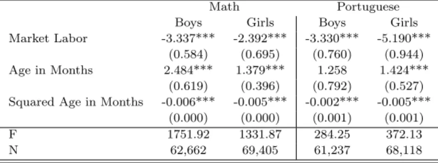
Tables 12 and 13 present coefficient estimates on the paired sample that attempt to isolate
the effect of a child starting to work and a child stopping working. In order to accomplish
this, the estimation presented in Table 12, ’Ins’, selects all those who did not work in the
first period of observation (t) and compares those that continued without working in the
next window of observation (t+ 2) to those were working in the next window of observation
(t+ 2). Table 13, ’Outs’, does the opposite: it considers all those that were observed to
be working in the first period (t) and compares those that remained working in the next
period of observation (t + 2) to those that were no longer working in the next period of
observation. The coefficient estimates for the child labor variable presented in Table 12 for
the ’ins’ are all negative and significant at the one percent level, similar to Table 9, but
the point estimates are larger.16 The marginal impact of these new estimates now range
from 6.2% (girls math) to 10.6% (girls Portuguese) of a standard deviation decline in test
score. Interpreting these in terms of average annual increases in test scores reveals that the
15
The negative effect dominates for those whose test scores are above: 171.1 for boys math; 187.9 for girls math; 173.1 for boys Portuguese; 113.8 for girls Portuguese. All well below their respective means.
16
impact of starting to work is equivalent to roughly one half to a whole year of learning loss.
The coefficient estimates for the child labor variable presented in Table 13 for the ’outs’ are
all negative and significant at the one percent level, similar to Table 9, but again the point
estimates are larger. The marginal impact of the estimates now range from 6.7% (boys math)
to 19.0% (girls Portuguese) of a standard deviation decline in test score of roughly one half
to almost two years of learning loss for those that remain in the labor market compared to
those who exit.
[INSERT TABLE 12 AND 13 AROUND HERE]
The ‘In’ and ‘Out’ coefficient estimates have similar magnitudes and we cannot reject that
they are statistically equal to each other. Therefore there is not evidence of heterogeneity
between moment into or out of the labor market. This could suggest that transitions into and
out of the labor market may be due to individual idiosyncratic shocks that are orthogonal
to proficiency.
5.3
Exposure and lingering e
ff
ects of child labor
We now turn to two questions that demand the use of the third ’three period’ sample. Recall
that this sample takes all of the children we observe in 6th grade in either 2007 or in 2008
and whom we observe in the next two consecutive years (regardless of progression through
the grades) and we compare scores in t and t+ 2. Table 14 presents estimates of ’exposure
effects’ and takes all children who are not working in the first observation year and compares
those who only work in the third year (group 1) to those who work in the second and
third years (group 2) to see if consecutive years of exposure have increasing or decreasing
marginal effects on the students’ test scores. For boys math scores the coefficient estimates
significant. Interestingly, the two year indicator variable coefficient is almost double the one
year estimate, suggesting that the effect is essentially linear. Each year of working leads
to about a 3.1 point drop in test scores. For the other regressions the effects could not be
separately identified perhaps due to the fairly small sample size we are now working with.
[INSERT TABLE 14 AROUND HERE]
Another question we seek to address using the three period sample is the question of
’lingering effects.’ In Table 15 we present coefficient estimates of regressions where we again
start with those that initially do not work and compare those that remain not working for
all three years to those that work in the second year but do not work in the third. The
question is if having worked in the past continues to depress a child’s test score or do they
‘catch up?’ From the results in Table 15 we find some evidence that the effects do linger
for boys as for math and Portuguese the coefficient estimates are negative and significant
(at the 10% level for math). For girls the point estimate for the math coefficient is negative
and of a similar magnitude to previous regressions but has a large standard error and is
not statistically significant while the Portuguese coefficient estimate is both very small and
insignificant.
[INSERT TABLE 15 AROUND HERE]
5.4
Robustness checks
We next conduct a series of robustness checks. The first set are described in Table 16:
using the three period sample we conduct a series of difference-in-difference estimates on the
relative test score increase over the first two years for kids with identical work experiences
impact of working in the third year for those with identical work histories.17 Below we show
the four subsamples we use to conduct the robustness checks. Those who did not work in
year t ort+ 1 (Treatment 001), those who worked in both yeart and year t+ 1 (Treatment
111), those who worked in year t but did not work in year t+ 1 (Treatment 101)and those
that did not work in year t but did work in year t+ 1 (Treatment 011). We will compare
the score trajectory between t and t+ 1 for all subsamples.18
[INSERT TABLE 16 AROUND HERE]
In each case we estimate our model for both boys and girls and for both math and
Portuguese for a total of 16 robustness tests. The results for boys are presented in Table
17 and the results for girls are presented in Table 18. In all cases but one the robustness
test yields the expected result: no difference in the test score progression. In one case the
math scores for boys is negative and significant. This could suggest that there could be
some selection on trends in scores: boys who observe their score progressing slowly select
into child labor or perhaps some correlation with unobserved prior work history.
[INSERT TABLE 17 AND 18 AROUND HERE]
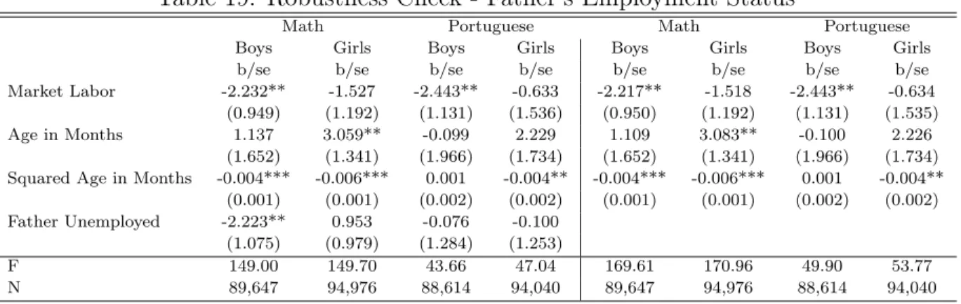
The final robustness check is on the effect of the time-variant employment status of the
father. As there are many missing observations and we do not have information on the
parents for 2008, the sample size has decreased considerably from the benchmark case on
the full pooled sample. For this reason we estimate the benchmark regression both without
and with the father’s employment status variable as a control using this sample.
Table 19 presents the result of the estimations of the benchmark model on the sample
17
We can only identify those with identicalobservedprevious work histories, therefore we cannot completely
exclude the possibility that unobserved work histories are correlated with future work histories. This could happen for children in households particularly sensitive to income shocks, for example.
18
of observations for which we have information on the employment status of the father both
including and excluding the father’s employment status as proxy for idiosyncratic economic
shocks to the household. We find that for boys the point estimates for both math and
Portuguese are statistically significant and larger than in the benchmark regression on the
pooled sample when father’s employment status is not included as a control. However, there
is almost no change in the size or significance of the variable when we control for father’s
employment status suggesting the fixed-effect estimator is not biased upward. For girls the
change in sample size causes the point estimates for both math and Portuguese to shrink
and loose significance relative to the benchmark case on the full sample, but again, there is
virtually no difference between the coefficient estimates from the regressions where father’s
employment status is excluded and included. These results suggest that our coefficient
estimates are not biased due to correlation with time variant idiosyncratic shocks to the
household.19
[INSERT TABLE 19 AROUND HERE]
5.5
Channels
Finally we explore potential channels through which child labor could be causing the
sup-pression of test scores. Table 20 has the results of the regression of the answers to the four
channels questions on the child labor indicator variable. For three of the variables there
is a positive and significant coefficient estimate for both boys and girls: missing classes,
completing homework at school, and turning in homework late. Boys (girls) are 6.4 (3.9)
percentage points more likely miss classes if they work while in school compared to students
19
who do not work, which translates to 29% (14%) more likely to miss classes. Similarly both
boys and girls are 2.2 percentage points more likely to complete their homework at school
(rather than at home) if they work, which translates to 8% (10%) more likely to complete
homework at home. Finally, boys (girls) are 3.1 (4.4) percentage points more likely to turn in
homework late if they work while in school, which translates to 5% (9%) more likely to turn
in homework late. These results suggest that the time burden of working while in school is
interfering with attendance and the careful and timely completion of assignments.
[INSERT TABLE 20 AROUND HERE]
6
Discussion and Conclusion
Working while in school has negative and lasting consequences for children who participate
in the labor market compared to those who do not. This paper finds negative and significant
impacts of working while in school on the math and Portuguese proficiency scores of children
enrolled in S˜ao Paulo municipal schools. The impacts are economically significant. The lower
bound of the average effects of working while in school hovers around 3 percent of a standard
deviation in math scores for boys and 6% for girls, and 5% for Portuguese for boys and 7%
for girls. When we isolate the effects for just those students who transition into child labor
we find negative effects of over 6% to over 10%. Extrapolating from the year to year average
gain in proficiency scores the average effect of transitioning to work while in school the effect
of working is equivalent to one quarter to an entire year of learning.
We show that these results are robust to idiosyncratic preferences and perform robustness
checks to rule out selection on idiosyncratic trends and economic shocks at the household
the effect lingers over time. We also find evidence that the negative effect of child labor while
in school operates through the interference in students’ study time allocation and habits such
as attending class, doing homework outside of class and turning in homework on time.
This is not to say that students that work are not optimizing. Their behavior could be
the consequence of an optimal decision including the cases where they have large discount
rates, are myopic about the future returns and simply prioritize current consumption as
some sociologists in Brazil have suggested. It is also possible that students lack information
about the true returns to learning in the adult labor market. Another explanation could
be that individuals are credit constrained and are unable to borrow against future earnings.
However, this individually rational (or boundedly rational) behavior of working while in
school is likely inefficient in the sense that the real cost to the individual exceeds the benefits
particularly in developing countries like Brazil where returns to education are very high.
Whatever the reason as student learning is highly correlated with adult outcomes as well as
economic growth, working while in school is likely inefficient.
Though it is tempting to suggest that the policy prescription is to prohibit working for
students, one must proceed with caution. It is possible that without the ability to work
while in school these students would drop out of school entirely. In general the findings of
this paper show that while learning is impaired by working, learning still occurs even when
the child works at the same time. This suggests that working and going to school is better
than not going to school at all. We are also unable to comment on other effects of working
while in school such as grade repetition and dropping out as we are able to study only those
that remain in school. Nevertheless, policy interventions that manage to keep kids in school
while curtailing their work activity have the potential of producing a dramatic improvement
References
Akabayashi, Hideo and George Psacharopolous, “The Trade-off Between Child
La-bor and Human Capital Formation: A Tanzanian Case Study.,” Journal of Development
Studies, June 1999, 35, 120–140.
Assaad, Ragui, Deborah Levison, and H. Dang, “How Much Work Is Too Much?
Thresholds in the Effect of Child Work on Schooling - The Case of Egypt,” 2005. mimeo.
, , and Nadia Zibani, “The Effect of Child Work on School Enrollment in Egypt.,”
Working Papers 0111, Economic Research Forum April 2001.
Baland, Jean-Marie and James A. Robinson, “Is Child Labor Inefficient?,”Journal of
Political Economy, August 2000, 108 (4), 663–679.
Basu, Kaushik, “Child Labor: Cause, Consequence, and Cure, with Remarks on
Interna-tional Labor Standards,” Journal of Economic Literature, September 1999, 37 (3), 1083–
1119.
, “A note on multiple general equilibria with child labor,” Economics Letters, February
2002,74 (3), 301–308.
and Pham Hoang Van, “The Economics of Child Labor,”American Economic Review,
June 1998, 88(3), 412–27.
and Zafiris Tzannatos, “The Global Child Labor Problem: What Do We Know and
Beegle, Kathleen, Rajeev Dehejia, and Roberta Gatti, “Why Should We Care About
Child Labor?: The Education, Labor Market, and Health Consequences of Child Labor,”
Journal of Human Resources, 2009, 44(4).
, Rajeev H. Dehejia, and Roberta Gatti, “Child labor and agricultural shocks,”
Journal of Development Economics, October 2006,81 (1), 80–96.
, , , and Sofya Krutikova, “The consequences of child labor : evidence from
longitudinal data in rural Tanzania,” Policy Research Working Paper Series 4677, The
World Bank July 2008.
Bezerra, M´arcio Eduardo, Ana L´ucia Kassouf, and Mary Arends-Kuenning, “The
impact of child labor and school quality on academic achievement in Brazil,”IZA
Discus-sion Paper 4062, 2009.
Canals-Cerda, Jose and Cristobal Ridao-Cano, “The dynamics of school and work in
rural Bangladesh,” 2004. Bla.
Dessy, Sylvain E., “A defense of compulsive measures against child labor,” Journal of
Development Economics, June 2000,62 (1), 261–275.
and Stephane Pallage, “Child labor and coordination failures,”Journal of Development
Economics, August 2001, 65 (2), 469–476.
Dumas, Christelle, “Does Work Impede Child Learning? The Case of Senegal,”Economic
Development and Cultural Change, 2012, 60 (4), 773 – 793.
Duryea, Suzanne, David Lam, and Deborah Levison, “Effects of economic shocks
on children’s employment and schooling in Brazil,” Journal of Development Economics,
Edmonds, Eric V., “Child Labor,” in T. Paul Schultz and John A. Strauss, eds.,
Hand-book of Development Economics, Vol. 4 ofHandbook of Development Economics, Elsevier,
December 2008, chapter 57, pp. 3607–3709.
and Nina Pavcnik, “Child Labor in the Global Economy,” Journal of Economic
Per-spectives, Winter 2005, 19(1), 199–220.
Ejrnæs, Mette and Claus C P¨ortner, “Birth order and the intrahousehold allocation of
time and education,”Review of Economics and Statistics, 2004, 86(4), 1008–1019.
Emerson, Patrick M. and Andr´e Portela Souza, “Is There a Child Labor Trap?
Inter-generational Persistence of Child Labor in Brazil,” Economic Development and Cultural
Change, January 2003, 51 (2), 375–98.
and , “Is Child Labor Harmful? The Impact of Working Earlier in Life on Adult
Earnings,” Economic Development and Cultural Change, 2011, 59 (2), 345 – 385.
and Shawn D. Knabb, “Opportunity, Inequality and the Intergenerational
Transmis-sion of Child Labour,”Economica, 08 2006, 73 (291), 413–434.
and , “Fiscal Policy, Expectation Traps, And Child Labor,” Economic Inquiry, 07
2007,45 (3), 453–469.
and , “Expectations, Child Labor and Economic Development,” 2008. Working Paper,
Department of Economics, Oregon State University.
Gunnarsson, Victoria, Peter F. Orazem, and Mario A. Sanchez, “Child Labor
and School Achievement in Latin America,” World Bank Economic Review, 2006,20 (1),
Hanushek, Eric A. and D. D. Kimko, “Schooling, Labor Force Quality and the Growth
of Nations,”American Economic Review, 2000, 90 (5), 1184–1208.
and L. Zhang, “Quality consistent estimates of international schooling and skill
gradi-ents,” Journal of Human Capital, 2009, 3 (2), 107–143.
Heady, Christopher, “The Effect of Child Labor on Learning Achievement,” World
De-velopment, February 2003, 31(2), 385–398.
Horowitz, Andrew W. and Jian Wang, “Favorite son? Specialized child laborers and
students in poor LDC households,” Journal of Development Economics, April 2004, 73
(2), 631–642.
Ilahi, Nadeem, Peter Orazem, and Guilherme Sedlacek, “The Implications of Child
Labor for Adult Wages, Income and Poverty: Retrospective Evidence from Brazil.,” 2001.
Working Paper, Iowa State University.
Orazem, Peter F. and Chanyoung Lee, “Lifetime Health Consequences of Child Labor
in Brazil.,” 2007. Working Paper, Department of Economics, Iowa State University.
Ponczek, Vladimir and Andre Portela Souza, “New Evidence of the Causal Effect of
Family Size on Child Quality in a Developing Country,” Journal of Human Resources,
2012,47 (1), 64–106.
Psacharopoulos, George and Harry Anthony Patrinos, “Family size, schooling and
child labor in Peru - An empirical analysis,” Journal of Population Economics, 1997, 10
Ravallion, Martin and Quentin Wodon, “Does Child Labour Displace Schooling?
Ev-idence on Behavioural Responses to an Enrollment Subsidy,” Economic Journal, March
Tables
Table 1: Full Sample - Descriptive Stats
Boys
Min Max Mean SD
Proficiency Math 0 411.87 219.00 43.63
Proficiency Portuguese 0 380.02 204.42 51.05
Market Labor 0 1 0.12 0.33
Chores 0 1 0.32 0.47
Age in Months 128 250 166.86 15.15
6th grade 0 1 0.53 0.50
7th grade 0 1 0.10 0.30
8th grade 0 1 0.37 0.48
Late Homework 0 1 0.58 0.49
Homework at School 0 1 0.27 0.45
Prepare for exam 0 1 0.70 0.46
Miss Classes 0 1 0.22 0.41
Father’s Unemployment 0 1 0.11 0.32
Girls
Min Max Mean SD
Proficiency Math 0 409.97 216.50 40.55
Proficiency Portuguese 0 381.03 218.60 49.20
Market Labor 0 1 0.06 0.23
Chores 0 1 0.56 0.50
Age in Months 119 249 164.64 14.45
6th grade 0 1 0.54 0.50
7th grade 0 1 0.10 0.29
8th grade 0 1 0.36 0.48
Late Homework 0 1 0.51 0.50
Homework at School 0 1 0.22 0.42
Prepare for exam 0 1 0.71 0.45
Miss Classes 0 1 0.27 0.44
Table 2: Paired Sample - Descriptive Stats
Boys
Min Max Mean SD
Proficiency Math 99.79 411.86 221.40 41.73
Proficiency Portuguese 0 380.0234 206.3126 49.98
Market Labor 0 1 0.11 0.32
Chores 0 1 0.32 0.46
Age in Months 128 241 167.35 14.75
6th grade 0 1 0.51 0.50
7th grade 0 1 0.0054 0.074
8th grade 0 1 0.48 0.49
Girls
Min Max Mean SD
Proficiency Math 108.13 409.97 218.96 38.63
Proficiency Portuguese 0 381.03 220.86 48.90
Market Labor 0 1 0.055 0.22
Chores 0 1 0.558999 0.49651
Age in Months 124 246 165.70 14.26
6th grade 0 1 0.51 0.50
7th grade 0 1 0.004 0.061
8th grade 0 1 0.48 0.49
Table 3: 3 Period Sample - Descriptive Stats
Boys
Min Max Mean SD
Proficiency Math 113.57 391.26 220.88 41.90 Proficiency Portuguese 0 352.60 206.61 48.39
Market Labor 0 1 0.07 0.26
Chores 0 1 0.34 0.47
Age in Months 135 232 170.94 16.27
6th grade 0 1 0.50 0.50
7th grade 0 1 0.01 0.08
8th grade 0 1 0.50 0.50
Girls
Min Max Mean SD
Proficiency Math 108.13 395.50 217.22 38.77 Proficiency Portuguese 0 380.02 218.75 46.93
Market Labor 0 1 0.04 0.19
Chores 0 1 0.58 0.49
Age in Months 131 267 169.18 15.42
6th grade 0 1 0.50 0.50
7th grade 0 1 0.00 0.07
Table 4: Transition Matrix - Market Labor - Full Sample
Boys
t+1
Not Working Working Total
t
Not Working 30,592 4,412 35,004
87.40% 12.60%
Working 2,734 1,690 4,424
61.80% 38.20%
Total 33,326 6,102 39,428
84.52% 15.48%
Girls
t+1
Not Working Working Total
t
Not Working 32,906 2,267 35,173
93.55% 6.45%
Working 1,251 485 1,736
72.06% 27.94%
Total 34,157 2,752 36,909
92.54% 7.46%
Table 5: School Attendance and Child Labor - City of S˜ao Paulo 2010
Number and Proportion of 10 to 17 Year Olds
Boys Girls Total
Only School 590.19 591.004 1,181,194
85.39% 86.63% 86.01%
Only Work 17.146 11.37 28.516
2.48% 1.67% 2.08%
School and Work 43.084 36.674 79.758
6.23% 5.38% 5.81%
No School and No Work 40.773 43.155 83.928
5.90% 6.33% 6.11%
Total 691.193 682.203 1,373,396
100% 100% 100%
Source: IBGE Demographic Census 2010.
Table 6: School Enrollment by Grade and School System - City of S˜ao Paulo 2010
Municipal Schools State Schools Private Schools Total
6th Graders 94.532 64.243 37.893 196.7
48.07% 32.67% 19.27% 100%
7th Graders 92.125 60.03 36.572 188.7
48.81% 31.81% 19.38% 100%
8th Graders 100.742 58.46 34.698 193.9
51.96% 30.15% 17.89% 100%
Total 287.399 182.733 109.163 579.3
49.61% 31.54% 18.84% 100%
Table 7: School Attendance by Grade and School System - City of S˜ao Paulo 2010
Public Private Total
Not Work Work Not Work Work Not Work Work
6th Graders 132.838 9.529 33.448 346 166.286 9.875
93.31% 6.69% 98.98% 1.02% 94.39% 5.61%
7th Graders 117.233 12.628 28.962 658 146.195 13.286
90.28% 9.72% 97.78% 2.22% 91.67% 8.33%
8th Graders 132.808 34.124 34.742 1.404 167.55 35.528
79.56% 20.44% 96.12% 3.88% 82.51% 17.49%
Total 382.879 56.281 97.152 2.408 480.031 58.689
87.18% 12.82% 97.58% 2.42% 89.11% 10.89%
Source: IBGE Demographic Census 2010.
Table 8: Occupational Distribution (%) - 2010
Sao Paulo Public School Students: 6th, 7th, and 8th Graders
Office Work 14.83%
Services and Retail Vendors 25.35%
Industry 23.53%
Domestic services, street vendors, car washers, and others 26.08%
Military Service Occupations 10.21%
Table 9: Benchmark Regressions
Full Sample Paired Sample
Math Portuguese Math Portuguese
Boys Girls Boys Girls Boys Girls Boys Girls
Market Labor -1.278*** -1.464*** -1.811*** -3.348*** -1.506*** -1.566*** -1.592*** -3.951***
(0.347) (0.458) (0.463) (0.630) (0.445) (0.568) (0.583) (0.774)
Age in Months 2.127*** 1.654*** 1.631** 1.686*** 2.350*** 1.381*** 1.346* 1.373***
(0.561) (0.347) (0.729) (0.470) (0.590) (0.392) (0.758) (0.522)
Squared Age in Months -0.006*** -0.005*** -0.003*** -0.005*** -0.006*** -0.005*** -0.002*** -0.005***
(0.000) (0.000) (0.001) (0.001) (0.000) (0.000) (0.001) (0.001)
F 1938.69 1449.57 334.15 426.14 1870.48 1371.13 301.01 382.21
N 191,494 190,067 186,035 185,860 80,260 82,485 78,109 80,693
Table 10: Interacting with age - first observ.
Math Portuguese
Boys Girls Boys Girls
Market Labor -5.098 -0.278 -7.167 6.879
(7.086) (9.341) (9.379) (12.786)
Age in Months 2.367*** 1.378*** 1.372* 1.348***
(0.591) (0.393) (0.759) (0.523)
Squared Age in Months -0.006*** -0.005*** -0.002*** -0.005***
(0.000) (0.000) (0.001) (0.001)
Market Labor×Age (1st Obs.) 0.023 -0.008 0.035 -0.069
(0.045) (0.060) (0.060) (0.082)
F 1662.64 1218.75 267.60 339.82
N 80,260 82,485 78,109 80,693
Table 11: Interacting with proficiency score - first observ.
Math Portuguese
Boys Girls Boys Girls
Market Labor 8.393*** 20.479*** 20.265*** 5.121
(2.744) (3.577) (2.636) (3.688)
Age in Months 2.377*** 1.401*** 1.391* 1.380***
(0.590) (0.392) (0.757) (0.522)
Squared Age in Months -0.006*** -0.005*** -0.002*** -0.005***
(0.000) (0.000) (0.001) (0.001)
Market Labor×Port. Score -0.117*** -0.045**
(0.014) (0.018) Market Labor×Math Score -0.049*** -0.109***
(0.013) (0.017)
F 1664.29 1224.03 276.18 340.47
Table 12: Ins - effect of entering the labor market
Math Portuguese
Boys Girls Boys Girls
Market Labor -3.337*** -2.392*** -3.330*** -5.190***
(0.584) (0.695) (0.760) (0.944)
Age in Months 2.484*** 1.379*** 1.258 1.424***
(0.619) (0.396) (0.792) (0.527)
Squared Age in Months -0.006*** -0.005*** -0.002*** -0.005***
(0.000) (0.000) (0.001) (0.001)
F 1751.92 1331.87 284.25 372.13
N 62,662 69,405 61,237 68,118
Table 13: Outs - effect of leaving the labor market
Math Portuguese
Boys Girls Boys Girls
Market Labor -2.765** -5.318** -3.784** -9.312***
(1.336) (2.164) (1.819) (2.906)
Age in Months -0.108 -12.921** 0.776 -14.027*
(1.975) (5.953) (2.612) (7.759)
Squared Age in Months -0.003** -0.004** -0.000 0.000
(0.001) (0.002) (0.002) (0.002)
F 126.04 47.43 20.71 15.44
N 5,908 2,515 5,725 2,442
Table 14: Exposure effects
Math Portuguese
Boys Girls Boys Girls
One year in the labor market -3.240** -1.174 -3.341** -3.288
(1.389) (1.695) (1.644) (2.046)
Two years in the labor market -6.206*** -3.817 0.248 -6.950
(2.271) (3.632) (2.703) (4.340)
Age in Months 3.967** 1.239** 1.349 0.715
(1.940) (0.622) (2.265) (0.731)
Squared Age in Months -0.005*** -0.003*** -0.003** -0.003***
(0.001) (0.001) (0.001) (0.001)
F 251.90 182.68 74.66 93.72
N 13,154 13,287 12,815 12,995
Table 15: Lingering effects
Math Portuguese
Boys Girls Boys Girls
In the market in the previous year -3.507* -3.869 -4.649** -0.431
(1.905) (2.446) (2.211) (2.896)
Age in Months 4.461* 1.139* 3.356 0.897
(2.578) (0.636) (2.979) (0.744)
Squared Age in Months -0.005*** -0.003*** -0.003** -0.004***
(0.001) (0.001) (0.001) (0.001)
F 250.33 193.17 79.74 102.55
Table 16: Robustness check samples
Treatment 001 Treatment 111
Periods t t+ 1 t+ 2 Periods t t+ 1 t+ 2
Treatment Not Working Not Working Working Treatment Working Working Working
Comparison Not Working Not Working Not Working Comparison Working Working Not Working
Treatment 101 Treatment 011
Periods t t+ 1 t+ 2 Periods t t+ 1 t+ 2
Treatment Working Not Working Working Treatment Not Working Working Working
Comparison Working Not Working Not Working Comparison Not Working Working Not Working
Table 17: Robustness checks - Boys
Treatment 001 Treatment 111 Treatment 101 Treatment 011
Math Portguese Math Portguese Math Portguese Math Portguese
Treatment 001 -2.846** -1.786
(1.350) (1.668)
Treatment 111 -2.978 1.991
(4.367) (5.896)
Treatment 101 -0.674 -3.313
(3.527) (4.323)
Treatment 011 -2.633 3.919
(2.539) (3.168)
Age in Months 2.279*** 2.760*** 4.545 -2.924 2.710 1.356 2.809 -0.054
(0.808) (1.011) (3.169) (4.578) (2.131) (2.617) (1.935) (2.424)
Squared Age in Months -0.006*** -0.009*** -0.010 -0.009 -0.008 -0.009 -0.008 -0.003
(0.002) (0.003) (0.008) (0.011) (0.006) (0.007) (0.005) (0.007)
F 76.46 29.91 3.75 1.46 4.20 2.65 6.70 2.36
N 11,829 11,514 500 482 947 915 1,236 1,187
Table 18: Robustness checks - Girls
Treatment 001 Treatment 111 Treatment 101 Treatment 011
Math Portguese Math Portguese Math Portguese Math Portguese
Treatment 001 -0.849 -2.116
(1.591) (1.997)
Treatment 111 2.653 2.262
(8.165) (10.173)
Treatment 101 4.326 -3.024
(5.197) (7.150)
Treatment 011 -2.506 1.152
(4.178) (6.054)
Age in Months 3.139*** 2.613*** 4.167 -7.944 5.495* -0.739 -0.422 4.044
(0.760) (0.972) (5.237) (6.538) (3.008) (4.958) (3.073) (4.569)
Squared Age in Months -0.009*** -0.009*** -0.012 0.022 -0.018** -0.003 0.003 -0.006
(0.002) (0.003) (0.015) (0.019) (0.008) (0.011) (0.008) (0.011)
F 38.64 45.57 1.33 0.48 3.55 0.58 2.04 0.82
Table 19: Robustness Check - Father’s Employment Status
Math Portuguese Math Portuguese
Boys Girls Boys Girls Boys Girls Boys Girls
b/se b/se b/se b/se b/se b/se b/se b/se
Market Labor -2.232** -1.527 -2.443** -0.633 -2.217** -1.518 -2.443** -0.634
(0.949) (1.192) (1.131) (1.536) (0.950) (1.192) (1.131) (1.535)
Age in Months 1.137 3.059** -0.099 2.229 1.109 3.083** -0.100 2.226
(1.652) (1.341) (1.966) (1.734) (1.652) (1.341) (1.966) (1.734)
Squared Age in Months -0.004*** -0.006*** 0.001 -0.004** -0.004*** -0.006*** 0.001 -0.004**
(0.001) (0.001) (0.002) (0.002) (0.001) (0.001) (0.002) (0.002)
Father Unemployed -2.223** 0.953 -0.076 -0.100
(1.075) (0.979) (1.284) (1.253)
F 149.00 149.70 43.66 47.04 169.61 170.96 49.90 53.77
N 89,647 94,976 88,614 94,040 89,647 94,976 88,614 94,040
Table 20: Channels
Miss Classes Prepare for exam Homework at school Late homework
Boys Girls Boys Girls Boys Girls Boys Girls
Market Labor 0.064*** 0.039*** 0.003 -0.003 0.022*** 0.022*** 0.031*** 0.044***
(0.006) (0.008) (0.006) (0.008) (0.006) (0.008) (0.007) (0.009)
Age in Months 0.003 0.012** 0.006 -0.005 0.008 0.006 0.008 0.013*
(0.009) (0.006) (0.009) (0.006) (0.010) (0.006) (0.011) (0.007)
Squared Age in Months -0.000*** -0.000*** 0.000 0.000*** -0.000** -0.000*** -0.000 -0.000*
(0.000) (0.000) (0.000) (0.000) (0.000) (0.000) (0.000) (0.000)
F 125.09 794.06 1715.58 1701.32 185.65 156.31 130.36 97.16