ASSOCIAÇÃO DE POLITÉCNICOS DO NORTE
(APNOR)
INSTITUTO POLITÉCNICO DE BRAGANÇA
The Impact of Oil shocks on Macroeconomic indicators: Evidence
from Belarus and Portugal
Volha Pleskatsevich
Final Dissertation submitted to
Instituto Politécnico de Bragança
To obtain the Master Degree in Management, Specialisation in Business
Management
Supervisors:
Nuno Filipe Lopes Moutinho
Andrei Chaplianski
ASSOCIAÇÃO DE POLITÉCNICOS DO NORTE
(APNOR)
INSTITUTO POLITÉCNICO DE BRAGANÇA
The Impact of Oil shocks on Macroeconomic indicators: Evidence
from Belarus and Portugal
Volha Pleskatsevich
Supervisors:
Nuno Filipe Lopes Moutinho
Andrei Chaplianski
Abstract
Nowadays oil have a significant impact in our daily life and the fluctuations in oil price are extremely worrisome for both country producers and country consumers, and also significantly affect both. Due to the fact that not only a decrease, but also an increase in oil prices leads to significant macroeconomic changes, the contemporary situation on the world markets can lead to a lot of tangible consequences both at the global, regional and country levels. Here we want to understand the dependence of the main macroeconomic indicators of two non-producer’s countries on the world oil prices. Because Belarus and Portugal have different macroeconomic backgrounds, it is supposed that a change in oil prices will have different effects in the economy of each country. The aim of this study is to analyse the relationship between oil prices and main macroeconomic indicators of Belarus and Portugal. In this thesis we use vector autoregressive models to study the direction and strength of the relationship between these factors.
we show that the change in oil prices has a tangible impact on the economic development of Portugal and Belarus. we have perceived a negative impact in macroeconomic indicators related with a rising in oil prices. In this study we find that oil price shocks have a deeper effect on the Portuguese economy than on the Belarusian economy. The oil prices have a negative impact on the macroeconomic indicators of both countries, but they are deeper in Portugal. On average, there is a more negative impact in short time, which weaken over the years.
Resumo
Hoje em dia o petróleo tem um impacto significativo na vida diária e as flutuações no preço do petróleo são extremamente preocupantes quer para países produtores como para países consumidores, pois afeta significativamente ambos. Devido ao fato de que não apenas uma redução, mas também um aumento nos preços do petróleo induzir mudanças macroeconómicas significativas, a situação contemporânea nos mercados mundiais pode levar a muitas consequências tangíveis tanto a nível global, regional e nacional. Neste trabalho pretendo perceber a dependência dos principais indicadores macroeconómicos de dois países não produtores face aos preços mundiais do petróleo. Dado que a Bielorrússia e Portugal têm origens macroeconómicas diferentes, supõe-se que uma alteração nos preços do petróleo terá efeitos diferentes na economia de cada país. O objetivo deste estudo é analisar a relação entre os preços do petróleo e os principais indicadores macroeconómicos da Bielorrússia e de Portugal. Nesta tese, são utilizados modelos vetoriais autoregressivos para estudar a direção e a força da relação entre esses fatores.
Neste sentido, apresento evidência de que a mudança nos preços do petróleo tem um impacto tangível no desenvolvimento económico de Portugal e da Bielorrússia. Também foi percebido um impacto negativo nos indicadores macroeconómicos relacionados com o aumento dos preços do petróleo. Neste estudo, considero que os choques nos preços do petróleo têm um efeito mais profundo na economia portuguesa do que na economia bielorrussa. Os preços do petróleo têm um impacto negativo nos indicadores macroeconómicos dos dois países, mas são mais profundos em Portugal. Em média, há um impacto mais negativo no curto prazo, que enfraquece com o decorrer dos anos.
Palavras-chave: Preço do petróleo, Indicadores macroeconómicos, Modelo VAR, Economia
Реферат
В настоящее время нефть оказывает значительное влияние на нашу повседневную жизнь, а
колебанияценнанефтьявляютсячрезвычайнотревожнымикак длястрал-производителей,так
идлястран-потребителей,атакжесущественновлияютинатех,инадругих. Всвязистем,что
падениеценнанефть,какиихрост,приводиткзначительныммакроэкономическимизменениям,
нынешняяситуациянамировомрынкенеизбежноприведеткрядуощутимыхпоследствийкакна
глобальном,такинарегиональномуровнях.Вработемыпроисследовализависимостьосновных
макроэкономических показателей двух стран-импортеров нефти от мировых цен на нефть.
ПосколькууБеларусииПортугалииразныемакроэкономическиефоны, смеюпредположить, что
изменениеценнанефтьбудетиметьразныепоследствиядляэкономикикаждойстраны.Целью
данного исследования является анализ взаимосвязи между ценами на нефть и основными
макроэкономическимипоказателямиБеларусииПортугалии.Вданнойдиссертациияиспользую
моделивекторной авторегрессии для изучения направления и силы взаимосвязи междуэтими
факторами.
Мы показали, что изменение цен на нефть, несомненно, оказывает ощутимое влияние на
экономическое развитие Португалии и Беларуси. Мы также выявили, что скачки цен на нефть
оказывают более глубокое влияние на португальскую экономику, чем на экономику Беларуси.
Ценынанефтьотрицательносказываютсянамакроэкономическихпоказателяхобеихстран,но
вПортугалииониболееощутимы. Всреднемзакороткоевремянаблюдаетсяболеенегативное
влияние,котороеослабеваетвтечениемвремени.Этаситуацияможетбытьсвязанасбольшей
открытостьюпортугальскойэкономикикмеждународнойторговлеиеебольшейзависимостьюот
ценнанефть,торгуемыхнамеждународныхрынках.
Ключевые слова:цены на нефть, экономический рост, VAR-модель, экономика Португалии,
Acknowledgements
I would like to express my sincere thanks to IPB for my education and to the professors of this institute for a permission to define the thesis. The knowledge and the skills that we acquired throughout the whole period of education are an indispensable component of my future career.
Especially thanks to my supervisors, professor Nuno Filipe Lopes Moutinho and professor Andrei Chapliansky, for their support, companionship, calmness, professionalism, and competence during my work. They shared their experience with me and we have learned a lot of new things. Also, deep gratitude to the staff of IPB, mainly professor Paula Odete Fernandes and the program coordinator from BSEU, professor Olga Morozevich, for their support, kindness and help in different situations.
Special thanks to international relation office in IPB, whose employees showed their professionalism and responsiveness to me during the period of education.
Abbreviations and Acronyms
ADF - Augmented Dickey-Fuller unit root test AIC - Akaike information criterion
Chi-sq - Chi-squared test CPI - Consumer price index
EXP - Exports of goods and services FDI - Foreign direct investment FPE - Final prediction error
GDP - Gross Domestic Product rate HQ - Hannan-Quinn information criterion IEA - International Energy Agency INF - Inflation rate
IRF - Impulse Response Function JB - Jarque-Bera test
LR - Likelihood-ratio test statistic
OIL - Crude oil price in international market
OPEC - the Organization of the Petroleum Exporting Countries PP - Phillips and Perron unit root test
Prob - Probability
Table of contents
1.Literature review ... 4
1.1. Oil Price and some Historical Evidence ... 4
1.2. Oil Shocks and the Labour Market ... 8
1.3. Oil shocks and the stock market ... 9
1.4. Oil shocks and Inflation ... 10
2.Research Methodology ... 12
2.1. Objective of the study and Research Hypotheses ... 12
2.2. Description of Data Analysis... 12
2.3. Description of Data Collection ... 13
3.Empirical Results Analysis ... 16
3.1. Sample Characterisation... 16
3.2. Stationarity test ... 20
3.3. Number of Lags ... 21
3.4. Analysis of Data Quality ... 22
3.4.1. Normality Test ... 22
3.4.2. Autocorrelation Test ... 22
3.4.3. Heteroscedasticity Test ... 23
3.5. Granger Causality Test ... 24
3.6. VAR Analysis ... 25
3.6.1. Variance Decomposition ... 25
3.6.2. Impulse Response Function ... 27
Conclusions, Limitations and Future Research Lines ... 30
References ... 32
Appendix ... 37
Appendix 1: Macroeconomic Indicators ... 37
Appendix 2: Variance Decomposition ... 38
Appendix 3: Impulse Response Function ... 41
List of Figures
Figure 1. Oil prices changes and US recessions, 1947-75 ... 5
Figure 2. Evolution of Macroeconomic variables in Belarus ... 17
Figure 3. Evolution of Macroeconomic variables in Portugal ... 18
Figure 4. Oil price between 1960 and 2016 ... 19
Figure 5. Response of Belarus macroeconomic variables to oil price impulse ... 27
List of Tables
Table 1. Descriptive Statistics ... 17
Table 2. Correlation Matrix ... 19
Table 3. Stationarity tests ... 20
Table 4. Lag selection criteria ... 21
Table 5. Normality test ... 22
Table 6. Autocorrelation Tests ... 23
Table 7. Heteroscedasticity Tests ... 23
Table 8. Granger Causality Test ... 24
Introduction
Nowadays oil is a key energy factor in the global economy. Despite the noticeable growth in the popularity of alternative renewable natural sources, such as wind, water, nuclear and solar energy, oil still holds a dominant position in the global energy balance. According to the Statistical Review of World Energy 2017 (BP, 2017), oil was the most important type of energy consumed since the middle of the 20th century until now.
As this product plays an important role in the world economy, the level of prices for it is an important reference point for all countries of the world. Theoretically, low world oil prices are beneficial for oil-importing countries: the lower the price of oil, the cheaper the production, the higher the consumer activity, and, finally, the faster the rate of economic growth. On the contrary, high world oil prices are beneficial to oil-exporting countries: the higher the price of oil, the greater the income from exports, the higher the investment in infrastructure and the higher the welfare of the population of these states. The mechanism of world oil prices has undergone significant changes over the years. For a long time, pricing in this market was oligopolistic, but since 1986 oil price is based on a stock exchange market. In this market oil prices experience daily fluctuations and are formed under the influence of a wide range of fundamental, geopolitical, financial and other factors. Slight fluctuations in prices do not have a significant impact on the economies of oil-exporting countries, while sharp fluctuations in world oil prices can destabilize national economies.
In order to study the impact of changes in oil prices on the economies of Portugal and Belarus, one must understand that these two countries are developing in completely different economic conditions. Belarus is the only country from the former Soviet republics, which in part retain its reliance on Soviet economic methods. Belarus imports oil. However, oil in the country exists. Its reserves are very scarce and do not provide for the state's needs in full. All extracted oil is used and processed in Belarus, in addition, most of the oil is exported from Russia and Venezuela. It should be noted that the oil refining industry in Belarus is well developed and often oil is brought to the country for processing. Belarus is too much connected with Russia, and its economy is almost entirely on oil reserves. Due to the peculiarities of geographical location and weather conditions, alternative energy sources in Belarus are poorly developed. We can assume that the change in oil prices will really affect the Belarusian economy.
in Portugal, the leading ones were hydraulic - 42% of the total production, wind energy (27%), biomass (3%) and solar energy (1%). Secondly, oil import in the country is much more diversified. According to International Energy Agency, the main oil exporters for Portugal in 2016 were Russia, Angola, Saudi Arabia, Algeria. This makes this country more independent of oil than Belarus. Therefore, it can be assumed that oil prices have less influence on its economic development. As for oil prices themselves, as is known, they change quite a lot in the last period: in December 2017, for the first time in 2.5 years, they reached the level of $ 66 per barrel of Brent brand, having overcome the shock drop of 2014-2015. In the modern era of the globalization of economic relations, many factors influence the world prices of energy carriers and especially oil: global and local economic crises, the growth rates of large countries’ GDP, the revolutionary changes in oil production technology, as well as the fact that significant impact on the formation of world prices are made by OPEC and IEA decisions, political and military events, embargoes, etc. In these conditions, the forecasting of world oil prices on the basis of statistical data is practically not feasible, because qualitative factors largely determine the fluctuations and sharp leaps in the energy market.
Therefore, at a given time, when all the indicators change quickly and, often, unexpectedly, it is very important to be ready for change and to know what they can lead the economies of the countries. This is what determines the importance and relevance of my research.
The object of this study became the economies of Portugal and Belarus in the light of the main macroeconomic indicators and the impact of the fluctuations in world oil prices.
As a method of research, we use the Vector Autoregression (VAR) model. It is one of the most popular methods of analysing various economic impacts in empirical literature. VAR allows to evaluate several variables at once and takes into account their interaction. The popularity of this method is explained by the relative simplicity of use, as well as by the ability to determine the channels for spreading various shocks in the country's economy by means of impulse response functions and obtain an economic interpretation of the evaluation results.
Based on the information on the peculiarities of the economies of Belarus and Portugal, as well as previous studies on this issue by other scientists, we set for myself the main task of investigation the existence of oil price influence on the main macroeconomic indicators of Belarus and Portugal, and through them on the economic growth of these countries. It is also important to know the level of this influence, as well as the similarities and differences in the influence of this factor between the two countries.
In order to achieve the goal, we analyze if changes in oil prices significantly affect GDP, inflation, foreign direct investment, the level of investment and the unemployment rate of Belarus and Portugal. We also would like to analyze if the impact of oil prices in Belarus and Portugal is not the same due to the difference in economics.
1.
Literature review
1.1. Oil Price and some Historical Evidence
Today there is large number of studies about interconnection between the oil price and the economic growth of countries. Hamilton's work from 1983 is considered as a fundamental work about this issue and still very important for analysis of oil prices and their macroeconomic impact. In the paper, the author tried to prove the serious decline in the US economy after the Second World War with a sharp rise in oil prices. The economic depression of that time was expressed in the following: a sharp decline in the growth rate of real GNP (by 1.6 percentage points); increased more than twice the average rate of inflation; the highest unemployment rate for the last thirty years. Hamilton determined, that the US economic downturns appeared 3-4 quarters after the rise in oil prices, after what, 6-7 quarters later it is possible to observe recovery.
However, the author did not dare to say that the cause of all economic downturns after the Second World War were the jumps in oil prices. In the search for answers, Hamilton study the following: Hypothesis 1: Correlation is a historical coincidence. Hypothesis 2: Correlation is the result of the influence of third endogenous factors, which, presumably, could affect both the economic development of the country and the price of oil. Hypothesis 3: At least some factors of the US economic recession are caused by exogenous factors of rising oil prices.
On the Figure 1 we can see the changes in crude oil prices and US recessions, 1947-1975. Hypothesis 1 was eliminated almost immediately. Author safely connects the following historical events with the facts of the economic downturn in the United States: 1951-1952 - the Iranian nationalism; 1956-1957 - the Suez Crisis; 1969 - secular decline in US reserves; 1970 - the trans-Arabian pipeline; 1973 - the OPEC embargo; 1980 - beginning of Iran-Iraq war. These events can be safely considered the causes of depressive results in the US economy.
series in evidence prior to the oil price increases. As a result, evidence, that the above series carry reliable information about the increase in oil prices, were not found. Testing the hypothesis 3 showed that the timing, magnitude as well duration of the economical decreases after 1973 were more discernible with oil prices.
Source: Hamilton (1983, p.229).
Based on the work of Hamilton, Mork (1989) added data after the 1980s, which significantly reduced the impact of oil prices on the country's economic development. He also changed the research model somewhat, which more suited the selected data.
As a result, Mork came to the conclusion that, with an increase in oil prices, the model showed significantly different coefficients than when they were going down. The VAR was structurally stable across that breakpoint, and price increases Granger-caused output changes while price decreases did not (p-values of .001 and .152).
So, he came up with the asymmetric effects of oil prices changes, that he left without any advance in theoretical explanation of this fact. He also proved that oil prices downturn does not have statistically significance for the economy of the USA.
Jones, Leiby and Paik (2003) distinguished five direction of research when estimation the state of knowledge on the impact of oil prices fluctuations on the economic growth. The first of these was the mechanism for transferring the effects of a change in the level of oil prices to the economy at the micro-level (the use of disaggregated data at the firm level, theoretical models for different market set-ups, etc.). The second branch is connected with the fact that oil shocks often led to interference in monetary policy - a kind of indemnity issue. A number of authors believed that it was precisely
changes in monetary policy that led to stagflation, rather than shocks of oil prices (Hooker, 2002); Bernanke, Gentler and Watson (1997, pp 135) also attributed the deepening of stagflation to monetary policy, they argued that ”thеFedеralResеrvepоlicy is largеlyendogenоus duе to thе its
cоmmitmenttоmacroecоnоmic stabilization”. The third prospect expresses a detection stability of relations between GDP and oil prices over time. This idea was supported by many authors. Among others, Rotemberg and Woodford (1996) claimed that in the 1980s the nature of the relationships of oil prices and GDP changed. They relate this to the fact that it was at the beginning of this period (early 1980s) that OPEC lost control over the nominal price of oil and could no longer sustain its stability, which led to a momentary reaction of the nominal price of oil. In this regard, they decided that one of two options is correct: either oil prices ceased to Granger-cause GDP or the relations between them have become much more complicated (in comparison with the earlier linear dependence). The empirical studies of asymmetry in the oil-GDP relationship (Mork, 1989) are also related to this question. The fourth branch is linked to the so-called magnitude of the oil price-GDP relationship. As for the US economy, the empirical tests provide the negative relationship, as it as expected. The fifth area pays attention to the relationships of oil prices and stock market performance.
Olivier and Galí (2008) evaluated a hypothesis that results of the oil prices up goings were similar in 1970s as well as in 2000s, but the differences in the effects could be caused by faced the shocks of different format, like other raw materials prices in the 1970s and increase in productivity and world demand in the 2000s. This fact could noticeably misrepresent an assessment of influence of oil price shocks based on a simple examination of the movements in aggregate variables around each period. The scientists used structural VAR technics to evaluate this assumption identifying and estimating the effects of the price of oil: they needed to insulate the element of macroeconomic fluctuations connected with exogenous modifications in oil prices.
As a result, it was proved that, firstly, the consequences of sharp changes in oil prices also coincided with other significant shocks, which caused a difference in the results. Secondly, the impact of the oil prices themselves has changed over time: the influence on wages, prices, the volume of production and the level of unemployment has slowed.
The reasons for these changes were also revealed. One of them is real wage stiffness, ‘such rigidities are needed to generate the type of large stagflation in response to adverse supply’. It turned out that over time, consumption wages became more sensitive to the marginal rates of substitution (and hence to employment). In addition, increased confidence in monetary policy has also become the reason for measuring the reaction of the economy to oil price shocks. This could be proved by a simple formalization of the absence of a power of attorney and its influence on the boundary of volatility: the reaction of expected inflation to oil prices changes significantly decreased. The third identified cause was a significant reduction in the use of oil in production and in consumption. This decline was strong enough to reduce the merger of the change in oil prices.
erratic.
A number of scientists have faced the fact that the impact of world oil prices differs significantly from country to country. Burbidge and Harrison (1984) demonstrated that industrial production in the United States and Great Britain became subject to a significant impact of oil shocks, while for Japan, Germany and Canada, it is relatively small. Bjørnland (2000) study Norway, Germany, Great Britain, USA and Canada data and found that the effect of oil prices was positive only for Norway. Chuku et al. (2010) found that changes in oil prices are not determinative for the macroeconomic activity of the Nigerian economy. Cunado et al. (2015) note the impact of sharp fluctuations in oil prices on the economies of Asian countries (Japan, Korea, India and Indonesia) from 1974 to 2013. The results show that the economies of these countries are very sensitive to a sharp change in oil prices. Rautava (2002), Ito (2008) and Melnikov (2010) report on the positive impact of global oil price shocks in Russia. In the work of Sarzaeem (2005), it was shown that a sharp rise in oil prices leads to an increase in inflation and liquidity in Iran. In the works of Farzanegan and Markvard (2009) and Samadi et al. (2009), the negative impact of oil sharp fluctuations on Iran's economic growth was found. In work Mahregan and Salmani (2014) analysed the impact of sharp fluctuations in oil prices on Iran's economic growth with the help of the Markov model from 1987 to 2011. Their results show that the positive impact of a sharp rise in oil prices on Iran's economic growth is less than the negative impact of a sharp drop in oil prices on Iran's economic growth.
Usman et al. (2011) and Rafay and Farid (2015) in their works found negative reaction of such variables as employment and output on the raice of oil prices in Pakistan. It was also found that the short-term impact is significantly greater, than the long-term one.
Studying the economy of China, Shuping et al. (2012) not only discovered the effect of the volatility of oil prices on production, but also revealed the reasons for this influence. The first is the psychological expectation of economic growth by buyers, the second is the impact on monetary policy.
Some works (Mehrara and Oskoui, 2007; El-Anshasy and Bradley, 2012; Iwayemi and Fowowe, 2011) provide more specific information about oil price caused instability in oil-exporting countries. Mehrara and Oskoui (2007) and El-Anshasy and Bradley (2012) show that oil price shocks are the main cause of output fluctuations. On the contrary, Iwayemi and Fowowe (2011) and Isah et al. (2015) show that the impact of oil price shocks on Nigerian (a purely oil-exporting country) macroeconomic variables is low. However, Isah et al. (2015) proved the oil price impact on external reserves.
Also Korhonen and Ledyaeva (2009) split the impact of oil prices fluctuation on the for oil consuming countries and for oil producing countries. In the end they show that the influence is different: such countries as Russia and Canada - oil producers - gain profit from positive changes of oil price, while countries consumers, such as Switzerland, Japan, Germany and UK incur losses.
these relationships, scientists used the multivariate methodology of VAR. They singled out two time intervals for comparing the strength of the influence of the factors 1968-1985 and 1986-2005. As variables, average oil price, real Gross Domestic Product, Industrial Production Index, total employment, unemployment rate and the CPI-based inflation rate were chosen. As a result, they showed that the fluctuation in oil prices had a pronounced effect on the level of inflation in the country throughout the entire examined period and the unemployment rate in the interval from 1968 to 1985. The impulse response functions were extremely useful in analysing the adjustment and the initial impact of the variations in the price of oil. Thеу also found that oil prices induce persistent effects on unemployment and inflation rates, and not so persistent effects on total employment and GDP. Robalo and Salvado noted the ambiguity of the reaction of industrial production. In general, this method supported the idea previously mentioned in the literature: there is a weakening of the reaction of economic factors to oil shocks after 1985, and the adjustment becomes more rapid.
1.2. Oil Shocks and the Labour Market
Different ideas about the interrelation between oil price shocks and unemployment ere put forward. But the most common was the theory about the supply-side effect: when the price of oil is going up, the availability of oil as basic input in production is decreasing (Brown and Yücel, 1999). As a result, the growth of output is slowing down, real wage growth also decreases, as well as unemployment. Brown and Yücel (1999) describe this effect in the following way: the oil price jump reflects in slowing down of GDP growth, that leads to an upward trend in unemployment, which in turn drives to a further reduction in GDP growth. It continues unless unexpected inflation increases as much as GDP growth falls. The first reduction in GDP growth always comes together with a fall in labour productivity. And if the real wages do not fall as much as the reduction in labour productivity, companies will have to dismiss workers, that will lead to prolongation of GDP loses and unemployment growth. Brown and Yücel (2002) highlight only one situation, when a reduction in wages can help stabilize the situation on the labour market in this case - when unexpected inflation that is at least as great as the reduction in GDP growth.
on the change in the level of unemployment; the transmission mechanism of such shocks is the job finding rate; oil price shocks are complementary to the standard technological shocks and provide a new amplification mechanism of business cycle fluctuations in the context of the Pissarides’ model. Van Wijnbergen (1985) came up with the idea that oil price shocks have different impact on the labour market behaviour in different countries. Similarly, Dogrul and Soytas (2010), who examined relationship between oil prices, interest rate, and unemployment, doubted if the results of their studies can be implemented for other developing countries. Fawad Ahmad (2013) using the Toda-Yamamoto causality test was studying the dependence of the labour market on the oil price shocks and real interest rate in Pakistan. While he did not find and significant association between the labour market state and real interest rate, the dependence on the oil price was found. This evidence the possibility of application the previous researches regarding the relationship of these variables to developing countries.
1.3. Oil shocks and the stock market
There are no many researches about the correlation between the price of oil and the stock market fluctuations. Jones and Kaul (1996) examined if current and future changes in real cash flows and changes in expected returns can explain the reaction of the international stock market to the oil price changes. Studying the post-war period, they proved that oil shocks have a direct impact on the financial markets of Canada and the United States, but does not have such a strong influence on the stock market of the United Kingdom and Japan.
Huang, Masulis and Stoll (1996) tested the link between daily oil future returns and daily United States returns. Their results suggested that oil returns do lead some individual oil company stock returns, but oil future returns do not have much impact on general market indices.
Having selected for his study the period 1947-1996, Sadorsky (1999) demonstrated that the real profitability of shares is subject to great influence from the price of oil and its volatility. Notably, oil price fluctuations after the middle of 198os justified a large fraction of the forecast error variance in real stock returns than was received from the interest rates. Papapetrou (2001) using a VAR approach was testing the impact of oil shocks on different economic indicators in Greece and proved that oil prices have significant influence on employment rate, real economic activities and also the stock market.
More specifically, the relevant literature generates mixed views regarding the effect of such oil-price shocks on asset prices, such as stock prices. Kaul and Seyhun (1990) announced that correlation between oil-price volatility and stock prices is negative (Hong et al., 2002; Sadorsky, 1999; O'Neil et al., 2008; Park and Ratti, 2008). Papapetrou (2001) associates this negative effect with the impact of the negative impact of oil shocks on employment and production growth.
premiums as the main determinants of oil and gas stock returns. He was supported by Gogineni (2007) and Yurtsever and Zahor (2007). One of the hypotheses they proved was the one that states that the change in oil prices positively affects the prices in the stock market, if oil price shocks reflect changes in aggregate demand, but negatively associate with stock price, if they reflect changes in supply. They also demonstrated an asymmetry in the relationship of these indicators: an increase in the price of oil leads to a decline in prices in the stock market, but the decline in oil prices is not associated with a decline in the stock market prices. Wei (2003) stated that it was not the oil prices increase in the USA (1973-1974), that explained the US stock market prices fall.
Kilian (2009) did not support all the above scientists and argued that oil price shocks are an exogenous factor. Other scientists have stated that oil prices react to other factors that also affect the stock market (Barsky and Kilian, 2002, 2004; Hamilton, 2005; Kilian, 2008).
Economists must decompose aggregate oil price shocks into the structural factors that reflect the endogenous character of such shocks. This solves two problems at once, such as a lack of research on this issue, as well as a lack of existing studies to determine the impact of these shocks on the asset rate.. Kilian and Park (2008) demonstrated that the impact that have oil price fluctuations driven by global oil-specific demand shocks differs from the one that have oil price fluctuations caused by global supply shocks in the crude oil market.
1.4. Oil shocks and Inflation
LeBlanc and Chinn (2004) studied the impact of oil shocks on inflation between 1980 and 2001 in countries such as the United States, France, Germany, the United Kingdom and Japan. Their main conclusions were that an increase in the price of oil by 10% leads on average to an increase in inflation by 0.1-0.8 percentage points. At the same time, scientists did not notice a significant difference between the results obtained in the US and the EU.
There are several explanations for reducing oil price shocks after the 1980s. Blanchard and Gali (2007) suggested that such changes as decline in real wage rigidities, the higher credibility of monetary policy and the decrease in the share of oil consumption and in production could reduce oil shocks impact; Peersman (2009) linked it with the change in the oil price shocks (decrease in oil demand elasticity over time); higher energy efficiency of production processes, the price setting due to globalization and also the better conduct of monetary policy that help to reduce the impact of oil price shocks were suggested by Alvarez et al. (2009).
(2000-2015), scientists concluded the share of transport in the CPI basket and energy subsidies are the most robust factors in explaining cross-country variations in the effects of oil price shocks during this period.
When studying the impact of oil shocks on the economies of MENA-6 countries, it was proved that, both for oil importing countries (Tunisia, Morocco) and for oil exporting countries (Bahrain, Saudi Arabia), an increase in oil prices leads to depreciation currency, but only in the short term, the inflation situation has stabilized for six months already (Brini, Jemmali and Farroukh, 2016).
Using the data of 50 countries and the period of 2007-08 Habermeier et al. (2009) found high role on the monetary policy in defining the scale of pass-through of oil price fluctuation. They stated that two factors can lead to lower pass-through of a country: high independence of central bank and inflation targeting regime. De Gregorio et al. (2007) attributed pass-through decreasing to declining in oil intensity and the exchange rate pass-through degree. They found that advanced counties achieve is lower than in developing economies. Conversely, Álvarez et al. (2011) stated that with time oil price shocks have bigger effect on the EU countries, attributing this change to the higher expenditure share of households on refined oil products, whereas their indirect and second-round effects have decreased.
Zoli (2009) and Caceres et al. (2012), using Vector Autoregressions, affirmed that reaction of domestic inflation rate to a global change in oil prices in developing countries can be influenced by specific factors of the region. These authors examined the economies of the countries of Emerging Europe and Central Africa and found that while in Emerging Europe countries the global oil price is a significant factor in explaining the inflation fluctuations, in Central Africa the prices are mostly controlled.
In one of the most recent works on (this topic, presented by Gelos and Ustyugova (2017), data of advanced and developing countries is examined by country-by-country augmented Phillips curves for the period 2000-2010. Differently from other studies, their analysis determines the only that high fuel intensities and pre-existing inflation levels are the only significant factors explaining cross-country differences in the effects of food and oil price shocks. The conduct of monetary policy, including the existence of inflation targeting regimes, does not seem to be a major determinant of the degree of pass-through.
2. Research Methodology
2.1. Objective of the study and Research Hypotheses
This thesis studies the key macroeconomic indicators of Belarus and Portugal and their evolution over the last decades. Whereas the economic growth and population well-being have been influenced by international factors that both countries do not control, it is proposed to analyze how the price of oil has affected the economies of both countries.
The main purpose of my work is to investigate the relationship between the main macroeconomic indicators and also oil prices in two countries: Belarus and Portugal. It is also important to know the level of this influence, as well as the similarities and differences in the influence of this factor between the two countries.
The main hypothesis we propose is that changes in oil prices significantly affect GDP, inflation, foreign direct investment, the level of investment and the unemployment rate of Belarus and Portugal. It would also be interesting to verify if the impact of oil prices in Belarus and Portugal is not the same due to the difference in economics.
2.2. Description of Data Analysis
The basic VAR model that we used to analyse the effect of oil prices on the main economic indicators, was as follows:
𝑌𝑖𝑡 = 𝐴1𝑌𝑖𝑡−1+ 𝐴2𝑋𝑡−1+ 𝑣𝑡 (1)
Where:
𝒀𝒊𝒕: is the vector of endogenous variables for country i in period t;
𝑿𝒕−𝟏: is the vector of exogenous variables in period t-1;
𝒗𝒕: is the error vector under normal distribution.
In order to study the data, it is important to investigate some descriptive statistics and the correlation matrix and to verify the evolution of macroeconomic variables. The next step is the determination of the number of lags that it will be used. The lagging length will be chosen according to the Akaike Information Criteria. Then, in VAR model there are some assumptions that will be analyzed, such as the stationarity of the series, the absence of autocorrelation, the lack of heteroscedasticity, and the normality of the residues. There are some tests that can be performed to analyse these assumptions: Augmented Dickey–Fuller and Phillips and Perron unit root tests are performed to test the stationarity; the Jarque-Bera residual normality test is performed to test the normality; Breusch Godfrey test is performed to test the autocorrelation; White test is performed to test the heteroscedasticity.
After this analysis we will check the Granger Causality Test to study the cause-effect relationship between time series. Finally, in the analysis of the VAR model, we will examine the Impulse Response Function (IRF) to describe the impact of a dynamic series in response to some external shocks and the Variance Decomposition (VD) to determine how much of the variance of the predicted error of each variable can be attributed to exogenous shocks for other variables.
2.3. Description of Data Collection
In this thesis we choose to study the macroeconomic consequences of the oil price changes using VAR method in the Republic of Belarus and in Portugal. For the first country, we examine the data from 1991 until now since there is no data available before that period, because the country was not independent and was a former member of the Soviet Union. For the second, we examine data from 1970, near 4 years before a political revolution from a dictatorship regime to a political democratic regime. We only use annual data because it is not possible to use quarterly or monthly data to Belarus. So, it is used crude oil price and macroeconomic data from Belarus and Portugal. The variables used are the following:
• GDPit: GDP growth (annual %) for country i in period t - Annual percentage growth rate of
in the value of the products. It is calculated without making deductions for depreciation of fabricated assets or for depletion and degradation of natural resources. Source: World Bank national accounts data, and OECD National Accounts data files.
• UNEMPt: Unemployment rate, is the total (% of total labour force) (national estimate) for
country i in period t - Unemployment refers to the share of the labour force that is without work but available for and seeking employment. Source: International Labour Organization, ILOSTAT database.
• INFt: Inflation, consumer prices (annual %) for country i in period t - Inflation as measured by
the consumer price index reflects the annual percentage change in the cost to the average consumer of acquiring a basket of goods and services that may be fixed or changed at specified intervals, such as yearly. The Laspeyres formula is generally used. Source: International Monetary Fund, International Financial Statistics and data files. • EXPt: Exports of goods and services (annual % growth) for country i in period t - Annual
growth rate of exports of goods and services based on constant local currency. Aggregates are based on constant 2010 U.S. dollars. Exports of goods and services represent the value of all goods and other market services provided to the rest of the world. They include the value of merchandise, freight, insurance, transport, travel, royalties, license fees, and other services, such as communication, construction, financial, information, business, personal, and government services. They exclude compensation of employees and investment income (formerly called factor services) and transfer payments. Source: World Bank national accounts data, and OECD National Accounts data files.
• FDIt: Foreign direct investment, net inflows (% of GDP) for country i in period t - Foreign
direct investment are the net inflows of investment to acquire a lasting management interest (10 percent or more of voting stock) in an enterprise operating in an economy other than that of the investor. It is the sum of equity capital, reinvestment of earnings, other long-term capital, and short-term capital as shown in the balance of payments. This series shows net inflows (new investment inflows less disinvestment) in the reporting economy from foreign investors, and is divided by GDP. Source: International Monetary Fund, International Financial Statistics and Balance of Payments databases, World Bank, International Debt Statistics, and World Bank and OECD GDP estimates.
• OILt: Price of oil in period t – Oil price is the Crude oil, average spot price of Brent, Dubai
and West Texas Intermediate, equally weighed. Source: World Bank.
3. Empirical Results Analysis
In order to achieve the objectives of the thesis, we will have to use the VAR-model, which requires several conditions to be fulfilled by the variables. First, the data must be stationary, and secondly, the conditions of normality, heteroscedasticity and absence of autocorrelation must be met. But above all, we must choose the optimal lag length.
3.1. Sample Characterisation
In this study we will use the crude oil price in international market (OIL) some of the most relevant macroeconomic factors in a country, like Gross Domestic Product growth rate (GDP), Unemployment rate (UNEMP), Exports of goods and services growth rate (EXP), Inflation (INF), and Foreign direct investment (FDI). Their values can be seen in Appendix 1.
A brief analysis of the descriptive statistics of the variables for each of the countries, presented in Panel A and Panel B of Table 1, allows one to perceive the macroeconomic behaviour of each of the countries.
Table 1. Descriptive Statistics
Panel A: Descriptive Analysis in Belarus
EXP FDI GDP INF UNEMP OIL
Mean 4,19 2,04 3,34 214,92 2,11 51,49
Median 6,30 1,96 4,89 35,47 2,00 44,95
Maximum 33,90 6,48 11,45 2221,02 6,10 95,27
Minimum -22,40 0,07 -11,70 7,03 0,50 15,90
Std. Dev. 13,32 1,56 6,61 505,86 1,52 28,74
Skewness -0,01 0,89 -0,86 3,09 1,28 0,32
Kurtosis 3,49 3,72 2,89 11,91 4,18 1,61
Observations 24 24 24 24 24 24
Panel B: Descriptive Analysis in Portugal
EXP FDI GDP INF UNEMP OIL
Mean 5,19 2,17 2,72 9,41 7,09 40,69
Median 5,90 1,27 2,14 5,21 7,19 31,80
Maximum 32,97 10,16 12,61 28,78 16,18 95,27
Minimum -15,71 0,27 -4,35 -0,84 1,40 5,21
Std. Dev. 7,84 2,16 3,56 8,80 3,38 25,72
Skewness 0,07 1,60 0,41 0,85 0,73 0,80
Kurtosis 6,45 5,50 3,44 2,38 3,49 2,62
Observations 47 47 47 47 47 47
Source: Authors`s own-elaboration
Figure 2. Evolution of Macroeconomic variables in Belarus
Source: Authors`s own-elaboration
-40 -20 0 20 40
92 94 96 98 00 02 04 06 08 10 12 14 16 B_Exports_growth 0 1 2 3 4 5 6 7
92 94 96 98 00 02 04 06 08 10 12 14 16 B_FDI -12 -8 -4 0 4 8 12
92 94 96 98 00 02 04 06 08 10 12 14 16 B_GDP_Growth 0 500 1,000 1,500 2,000 2,500
92 94 96 98 00 02 04 06 08 10 12 14 16 B_Inflation 0 1 2 3 4 5 6 7
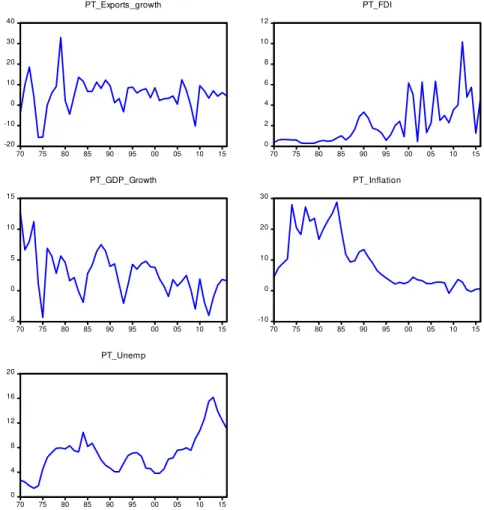
Figure 2 above shows the evolution of Belarus indicators. we can observe the decline in the level of inflation rates in recent times, as well as a slow decrease in the country's GDP growth after 2004. Exports and FDI are steadily growing. The evolution of the Portuguese macroeconomic variables can be verified in Figure 3. As we can see from the graphs, almost all the macroeconomic indicators of Portugal have a lot of fluctuation.
-20 -10 0 10 20 30 40
70 75 80 85 90 95 00 05 10 15 PT_Exports_growth 0 2 4 6 8 10 12
70 75 80 85 90 95 00 05 10 15 PT_FDI -5 0 5 10 15
70 75 80 85 90 95 00 05 10 15 PT_GDP_Growth -10 0 10 20 30
70 75 80 85 90 95 00 05 10 15 PT_Inflation 0 4 8 12 16 20
70 75 80 85 90 95 00 05 10 15 PT_Unemp
Figure 3. Evolution of Macroeconomic variables in Portugal
Source: Author`s own-elaboration
0 20 40 60 80 100
60 65 70 75 80 85 90 95 00 05 10 15
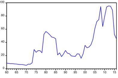
Figure 4. Oil price between 1960 and 2016
Source: Author`s own-elaboration
Table 2 shows the correlation matrix between the variables for both countries. From the correlation analysis, it can be seen that in both countries the time series of oil prices are correlated with macroeconomic indicators. The oil price is positively correlated with Belarus GDP growth, but negatively correlated with Portuguese GDP growth. Inflation rate is negatively related with oil price and foreign direct investment is positively correlated with oil price in both countries. Other correlations are presented in the table.
Table 2. Correlation Matrix
Panel A: Correlation Matrix in Belarus
EXP FDI GDP INF UNEMP OIL
EXP 1 0,37 0,58 -0,36 -0,09 0,15
FDI 0,37 1 0,25 -0,42 -0,14 0,61
GDP 0,58 0,25 1 -0,71 -0,19 0,29
INFLATION -0,36 -0,42 -0,71 1 -0,02 -0,44
UNEMP -0,09 -0,14 -0,19 -0,02 1 -0,48
OIL 0,15 0,61 0,29 -0,44 -0,48 1
Panel B: Correlation Matrix in Portugal
EXP FDI GDP INF UNEMP OIL
EXP 1 0,02 0,32 0,03 0,13 <0,01
FDI 0,02 1 -0,40 -0,52 0,44 0,55
GDP 0,32 -0,40 1 0,08 -0,52 -0,59
INFLATION 0,03 -0,52 0,08 1 -0,20 -0,23
UNEMP 0,13 0,44 -0,52 -0,20 1 0,79
OIL <0,01 0,55 -0,59 -0,23 0,79 1,00
Source: Authors`s own-elaboration
trends can be observed, such as a general increase or decrease in indicators over time and a correlation with the oil prices.
3.2. Stationarity test
Before further research, we first check the time series for stationarity. Thus, to confirm if the series used are stationary, tests are performed to the unit roots in order to measure the degree of integration of the series. It is important to note that a typical VAR model can only be constructed if the time series is stationary.
To check the stationarity, we conducted two tests: Augmented Dickey-Fuller (ADF, Dickey and Fuller, 1981) and Phillips and Perron (PP, Phillips and Perron, 1988) unit root tests. Their main difference is that PP does not require to select the level of serial correlation as in ADF, it takes the same estimation scheme as in ADF test, but corrects the statistic to conduct for autocorrelations and heteroscedasticity.
Table 3. Stationarity tests
Panel A: Stationary tests in
Belarus
EXP FDI GDP INF UNEMP OIL
ADF test
Level -3,92 -1,86 -1,85 -8,19 -3,48 -1,22
(0,01) (0,34) (0,35) (<0,01) (0,02) (0,65)
1st diference -3,46 -9,08 -5,29 -3,23 -5,13 -4,84
(0,02) (<0,01) (<0,01) (0,03) (<0,01) (<0,01) PP test
Level -3,76 -3,08 -1,85 -3,03 -3,39 -1,25
(0,01) (0,04) (0,35) (0,05) (0,02) (0,64)
1st diference -10,45 -9,91 -5,41 -6,08 -5,59 -4,84
(<0,01) (<0,01) (<0,01) (<0,01) (<0,01) (<0,01)
Panel B: Stationary tests in
Portugal
EXP FDI GDP INF UNEMP OIL
ADF test
Level -5,66 -2,43 -4,47 -1,12 -1,34 -1,84
(<0,01) (0,14) (<0,01) (0,70) (0,60) (0,36)
1st diference -6,22 -5,11 -5,51 -3,91 -4,77 -6,58
(<0,01) (<0,01) (<0,01) (<0,01) (<0,01) (<0,01) PP test
Level -5,32 -4,47 -4,49 -1,42 -1,63 -1,88
(<0,01) (<0,01) (<0,01) (0,56) (0,46) (0,34)
1st diference -20,73 -18,47 -8,80 -7,54 -4,74 -6,58
The Dickey–Fuller test involves fitting the regression model.
∆yt=ρyt−1+ (constant, time trend) +ut (2)
The Phillips–Perron test involves fitting (2), and the results are used to calculate the test statistics. They estimate not (2) but:
yt=πyt−1+ (constant, time trend) +ut (3)
The main hypothesis is the presence of a unit root, mathematically it is expressed in equality. If it is rejected, then there are no single roots and time series are stationary.
Table 4 show the results of stationary tests for each of the variables at the initial level and at the first difference. Although there are some variables stationary at the initial level, it can be observe that all variables – oil prices, GDP growth, unemployment, Inflation, exports of goods and services, and foreign direct investment of Portugal and Belarus – are integrated of order one. So, it can be concluded that all variables are stationary in first difference. In this way, we will use all variables as stationary in the first difference.
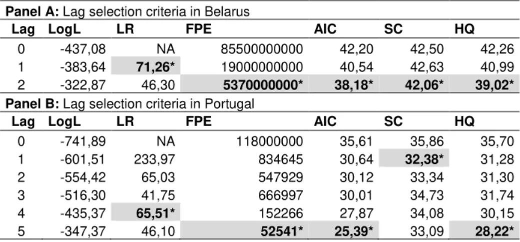
3.3. Number of Lags
To select the optimal VAR model, we need to determine the optimal number of lags. Since the choice of the optimal number of lags is relevant for the estimation of the VAR model, we use the following criteria: LR test statistic (LR); Final prediction error (FPE); Akaike information criterion (AIC); Schwarz information criterion (SC); Hannan-Quinn information criterion (HQ). If we analyse the data based in the Akaike information criterion, which is the best criteria, we would choose Lag 2 for Belarus and Lag 5 for Portugal. However, if we use other criteria we would get different conclusions, and because of the autocorrelation and heteroscedasticity test in the following section, we will use Lag 1 for Belarus and Lag 3 for Portugal.
Table 4. Lag selection criteria
Panel A: Lag selection criteria in Belarus
Lag LogL LR FPE AIC SC HQ
0 -437,08 NA 85500000000 42,20 42,50 42,26
1 -383,64 71,26* 19000000000 40,54 42,63 40,99
2 -322,87 46,30 5370000000* 38,18* 42,06* 39,02*
Panel B: Lag selection criteria in Portugal
Lag LogL LR FPE AIC SC HQ
0 -741,89 NA 118000000 35,61 35,86 35,70
1 -601,51 233,97 834645 30,64 32,38* 31,28
2 -554,42 65,03 547929 30,12 33,34 31,30
3 -516,30 41,75 666997 30,01 34,73 31,74
4 -435,37 65,51* 152266 27,87 34,08 30,15
5 -347,37 46,10 52541* 25,39* 33,09 28,22*
After the choice of the number of lags, we check the VAR stability condition which confirm that the model is stationary with 1 lag for Belarus and with 3 lags for Portugal.
3.4. Analysis of Data Quality
The appropriate use of the VAR model makes it necessary to comply with some requirements in addition to the stationarity of the series, like the absence of autocorrelation, the absence of heteroscedasticity, and the normality of the residuals. Because of that, we make the analysis of these assumptions in this point.
3.4.1. Normality Test
VAR models use the assumption of the normality of distributions, so specific tests for normality are needed. In this thesis we start doing a histogram method to test the normality of distribution. The histogram divides the series range (the distance between the maximum and minimum values) into a number of equal length intervals or bins and displays a count of the number of observations that fall into each bin. We also use the Jarque-Bera test (JB), that is a statistical test which verifies the observations errors on the normality. The null hypothesis of JB test is the normal distribution.
Table 5. Normality test
Panel A: Normality tests in Belarus
EXP FDI GDP INF UNEMP OIL Joint
Jarque-Bera 1,741 7,356 2,382 10,401 1,024 0,370 23,274
Probability 0,42 0,03 0,30 0,01 0,60 0,83 0,03
Panel B: Normality tests in Portugal
EXP FDI GDP INF UNEMP OIL Joint
Jarque-Bera 2,519 0,038 0,334 2,851 1,836 0,437 8,015
Probability 0,28 0,98 0,85 0,24 0,40 0,80 0,78
Source: Authors`s own-elaboration
Table 5 show the Jarque-Bera test coefficient and its p-value. If we use a level of significance of 5%, all p-values are greater in Portugal, but FDI and inflation are lower in Belarus. But if we use a level of significance of 1%, all variable will be greater than this level of significance in both countries. This means that for all variables the null hypothesis is not rejected and that all variables satisfy the condition of normal distribution. The problem related with inflation and unemployment in Belarus data at 5% is common in short sample series.
3.4.2. Autocorrelation Test
perceive the autocorrelation of the residuals, the test uses the auxiliary regression of the least-squares residuals of the original model for the factors of this model and the lag values of the residues. Further, for this auxiliary regression, the hypothesis of simultaneous equality to zero of all coefficients with lagged residues is verified. The test statistic has an asymptotic distribution. If the value of the statistics exceeds the critical table value, the autocorrelation is recognized as significant, otherwise it is insignificant. The null hypothesis of Breusch-Godfrey test (Autocorrelation LM Test) is the lack of autocorrelation, and the alternative hypothesis is its presence.
Table 6. Autocorrelation Tests
Panel A: Breusch-Godfrey Test in Belarus
Lags LM-Stat Prob
1 49,70 0,06
Panel B: Breusch-Godfrey Test in Portugal
Lags LM-Stat Prob
3 33,37 0,59
Source: Authors`s own-elaboration
Table 6 shows the results of autocorrelation tests. After testing the VAR models for Portugal with 3 lags and for Belarus with 1 lag, we find that in both cases the p-value exceeds 5%, which means that we accept the null hypothesis. In turn, this means that both models do not have autocorrelation, and therefore are suitable for further testing.
3.4.3. Heteroscedasticity Test
The analysis of VAR model implies to study the heteroscedasticity. In this way we use White test, that is necessary in order to proceed to hypotheses testing or forecasting. In this test the initial regression equation is evaluated and then an auxiliary equation is constructed for the dependence of the square of the residuals of the original equation on all independent variables, their squares and pairwise products. The null hypothesis of white test is that the residuals are homoscedasticity (or no heteroscedasticity), and the alternative hypothesis is that the residuals are heteroscedasticity.
Table 7. Heteroscedasticity Tests
Panel A: White Test in Belarus
Lags Chi-sq Prob
1 264,00 0,29
Panel B: White Test in Portugal
Lags Chi-sq Prob
3 786,90 0,21
After testing the VAR models for Portugal and Belarus we find that the p-value also exceeds 5% in the White test. It means that we accept the null hypothesis: both models do not have heteroscedasticity, and therefore are suitable for hypotheses testing and forecasting.
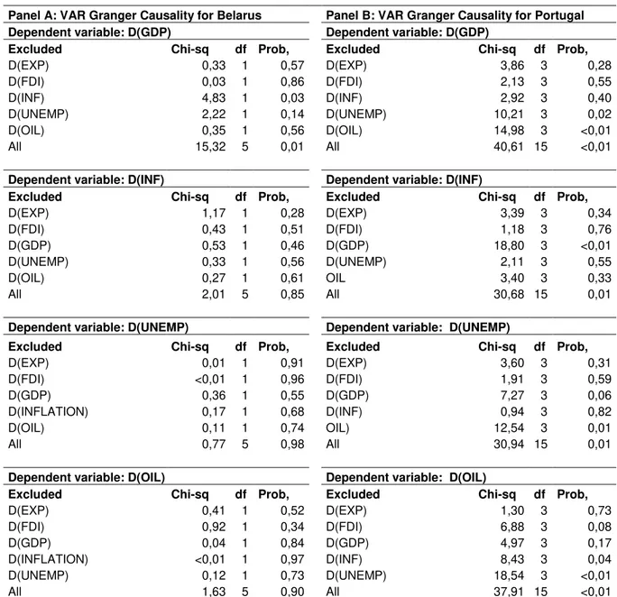
3.5. Granger Causality Test
Granger's test of causality is a procedure for checking the cause-effect relationship between time series. The idea of the test is that the values (changes) of one-time series, which is the cause of changes in another time series, must precede the changes of this time series, and besides, they should make a significant contribution to the forecast of its values.
Table 8. Granger Causality Test
Panel A: VAR Granger Causality for Belarus Panel B: VAR Granger Causality for Portugal
Dependent variable: D(GDP) Dependent variable: D(GDP)
Excluded Chi-sq df Prob, Excluded Chi-sq df Prob,
D(EXP) 0,33 1 0,57 D(EXP) 3,86 3 0,28
D(FDI) 0,03 1 0,86 D(FDI) 2,13 3 0,55
D(INF) 4,83 1 0,03 D(INF) 2,92 3 0,40
D(UNEMP) 2,22 1 0,14 D(UNEMP) 10,21 3 0,02
D(OIL) 0,35 1 0,56 D(OIL) 14,98 3 <0,01
All 15,32 5 0,01 All 40,61 15 <0,01
Dependent variable: D(INF) Dependent variable: D(INF)
Excluded Chi-sq df Prob, Excluded Chi-sq df Prob,
D(EXP) 1,17 1 0,28 D(EXP) 3,39 3 0,34
D(FDI) 0,43 1 0,51 D(FDI) 1,18 3 0,76
D(GDP) 0,53 1 0,46 D(GDP) 18,80 3 <0,01
D(UNEMP) 0,33 1 0,56 D(UNEMP) 2,11 3 0,55
D(OIL) 0,27 1 0,61 OIL 3,40 3 0,33
All 2,01 5 0,85 All 30,68 15 0,01
Dependent variable: D(UNEMP) Dependent variable: D(UNEMP)
Excluded Chi-sq df Prob, Excluded Chi-sq df Prob,
D(EXP) 0,01 1 0,91 D(EXP) 3,60 3 0,31
D(FDI) <0,01 1 0,96 D(FDI) 1,91 3 0,59
D(GDP) 0,36 1 0,55 D(GDP) 7,27 3 0,06
D(INFLATION) 0,17 1 0,68 D(INF) 0,94 3 0,82
D(OIL) 0,11 1 0,74 OIL) 12,54 3 0,01
All 0,77 5 0,98 All 30,94 15 0,01
Dependent variable: D(OIL) Dependent variable: D(OIL)
Excluded Chi-sq df Prob, Excluded Chi-sq df Prob,
D(EXP) 0,41 1 0,52 D(EXP) 1,30 3 0,73
D(FDI) 0,92 1 0,34 D(FDI) 6,88 3 0,08
D(GDP) 0,04 1 0,84 D(GDP) 4,97 3 0,17
D(INFLATION) <0,01 1 0,97 D(INF) 8,43 3 0,04
D(UNEMP) 0,12 1 0,73 D(UNEMP) 18,54 3 <0,01
All 1,63 5 0,90 All 37,91 15 <0,01
3.6. VAR Analysis
The VAR coefficients1 are not interpretable. The influence of one variable on another is not exhausted by the coefficient immediately before it. There is also an indirect influence through other variables. Interpretation of VAR is performed using the analysis of the Impulse Response Function (IRF) and the Variance Dispersion (VD).
3.6.1. Variance Decomposition
It is also important to analyse the Variance Decomposition. It determines how much of the variance of the predicted error of each variable can be attributed to shocks for other variables. In other words, the given analysis will allow to learn, what contribution change of one variable brings in change of another.
The variance decomposition allows one to estimate the contribution of the dispersion of one variable to the variance of the other. It provides information about the relative importance of each random perturbation in affecting the variables in the VAR system. The advantage of using this method of interpreting the results is that these contributions can be compared.
All results are presented in Appendix 2 and Table 9 only show the results of decomposition of the dispersion by the oil price factor. Analysing the data about the first difference, we can say that the impact of oil prices has a significantly different impact on macroeconomic indicators of Portugal and Belarus.
Panel A of Table 9 shows that, in the short run, that is year 2, impulse or innovation or shock to oil prices account 0,10% variation of the fluctuation in Belarus exportation growth, shock to oil prices can cause 1,81% fluctuation in foreign direct investment. Also, a shock of 1% in oil prices can cause 0,40% fluctuation in GDP growth, 0,55% fluctuation in inflation rate and 0,2% fluctuation in unemployment rate.
In the long run, that is year 10, impulse or innovation or shock to oil prices account 0,17% variation of the fluctuation in growth exportations, shock to oil prices can cause 1,51% fluctuation in foreign direct investment. Also, a shock of 1% in oil prices can cause 0,52% fluctuation in GDP growth, 0,56% fluctuation in inflation rate and 0,47% fluctuation in unemployment rate. Although the impact of oil prices in macroeconomic variables seems to be similar between short and long term, it seems to have little impact overall.
When we look into the Portuguese results, we see that the impact of oil prices increases a lot. Based on the Panel B of Table 5, we can say that a change in the variance of oil prices by 1% will lead to an increase 11,63% in the variance of Portugal's GDP in the short term, that is year 2. In the long run, year 10, this influence does not change much, and by the 10th period oil prices have an impact of 11,48%. Also for exportations we can observe a decrease in the influence of the change in oil
prices, since in the long run the percentage of the exponents of the dispersion of the variance decreases: from 14,98% in the short run to 12,11% in the long run.
Table 9. Variance Decomposition
Panel A: Variance Decomposition of Belarus
Variance
Decomposition of: D(EXP) D(FDI) D(GDP) D(INF) D(UNEMP)
Period
1 <0,01 <0,01 <0,01 <0,01 <0,01
2 0,10 1,81 0,40 0,55 0,20
3 0,16 1,43 0,39 0,55 0,41
4 0,16 1,43 0,51 0,55 0,46
5 0,16 1,54 0,51 0,56 0,47
6 0,16 1,57 0,51 0,56 0,47
7 0,16 1,58 0,52 0,56 0,47
8 0,16 1,58 0,52 0,56 0,47
9 0,17 1,58 0,52 0,56 0,47
10 0,17 1,58 0,52 0,56 0,47
Panel B: Variance Decomposition of Portugal
Variance
Decomposition of: D(EXP) D(FDI) D(GDP) D(INF) D(UNEMP)
Period
1 <0,01 <0,01 <0,01 <0,01 <0,01
2 14,98 2,96 11,63 0,50 3,46
3 13,97 2,50 8,73 0,47 3,86
4 14,37 9,91 8,23 4,68 3,68
5 12,07 10,20 10,42 4,67 6,16
6 12,21 10,07 11,01 4,61 8,96
7 11,92 10,24 10,75 4,40 9,55
8 11,56 10,67 10,57 4,32 9,79
9 12,46 10,82 11,78 4,42 9,79
10 12,11 11,10 11,48 4,71 10,10
Source: Authors`s own-elaboration
In the short run, that is year 2, impulse or innovation or shock to oil prices account 14,98% variation of the fluctuation in growth exportations, shock to oil prices can cause 2,96% fluctuation in foreign direct investment. Also, a shock of 1% in oil prices can cause 11,63% fluctuation in GDP growth, 0,50% fluctuation in inflation rate and 3,46% fluctuation in unemployment rate.
In the long run, that is year 10, impulse or innovation or shock to oil prices account 12,11% variation of the fluctuation in growth exportations, shock to oil prices can cause 11,10% fluctuation in foreign direct investment. Also, a shock of 1% in oil prices can cause 11,48% fluctuation in GDP growth, 4,71% fluctuation in inflation rate and 10,10% fluctuation in unemployment rate.
Although the results of oil prices impact are more relevant in Portugal, they have some more differences between short and long term effects.
3.6.2. Impulse Response Function
The impulse is a single perturbation, which is attached to one of the parameters. The Impulse Response function describes the response of a dynamic series in response to some external shocks. Shock refers to a one-stage change in exogenous variables, equal to their one standard deviation of the oscillations over the entire observed period. Basically, it shows how an increase in oil prices by 1% will change the macroeconomic indicators of countries. It is used the response to cholesky one standard deviation innovations.
Appendix 3 shows the results of an analysis of the impulse response function of exportations growth, GDP growth, inflation, unemployment and foreign direct investment. we can show that, for example, the change (which is as impulse or a shock) in the GDP growth has response of other variables, that is, if the GDP growth changes the other variables can also change or not change very much and eventually this effect tends to zero. Here we present and discuss the results of the response of macroeconomic variables to oil price changes.
Figure 5. Response of Belarus macroeconomic variables to oil price impulse
Source: Author`s own-elaboration
response in the second period and a slightly positive response in the following period. In the long term, the response to the oil price shock is practically non-existent.
In Figure 6 we can analyse Portuguese data and it is noted that a change in the price of oil gives a negative response to the growth rate of GDP and to the growth rate of exports. There is also a positive response in the inflation rate and in the unemployment rate when a shock occurs in oil price. During the period it is showed that there are several fluctuations in the responses of the macroeconomic variables to the oil price shocks.
From this analysis it seems to be concluded that oil price shocks have deeper effects on the Portuguese economy than on the Belarusian economy. Comparing the two countries, Portuguese macroeconomic indicators are more prone responding to oil shocks than Belarus variables. This situation may be related to the greater openness of the Portuguese economy to international trade and its greater dependence on the oil price traded in international markets.
Figure 6. Response of Portuguese macroeconomic variables to oil price impulse
Source: Author`s own-elaboration