Orlando C. Rodr´ıguez
1, Ant´onio J. Silva
1, Friedrich Zabel
1,S´ergio M. Jesus
11Instituto de Sistemas e Rob´otica, Campus de Gambelas, Universidade do Algarve,{orodrig,asilva,sjesus}@ualg.pt,fredz@wireless.com.pt
Current development of Internet access, together with available zero-cost Open Source applications (like, for instance, PHP, Python, etc.) can be integrated in order to minimize the constrains induced by the geographical separation of international centers, which collaborate in a given project. The advantage of such approach lies in the sharing of common analysis methods, without particular constrains to specific directions of analysis. The discussion presented in this paper describes the Time Variable Acoustic Propagation Model (TV-APM) web interface, which was created as a collaborative service of acoustic modeling for the participants of the PHITOM and UAN projects. This paper describes the general architecture of the interface, its current shortcomings and advantages, and presents a set of modeling results for short range acoustic propagation, which accounts for source–array and sea surface motion.
1
Introduction
The UAN project1is a research project approved within the
European Community’s 7th Framework Programme, whose main objective lies in the conception, development and test at sea of an innovative wireless underwater network integrat-ing submerged, terrestrial and aerial sensors for the protec-tion of off-shore and coastline critical infrastructures. The
PHITOM project2 is a research project, approved by the
Portuguese Foundation for Science Technology programme, which aims at developing and applying techniques of ocean acoustic tomography to the HF signals used in digital com-munications. The participants in both projects involve insti-tutions from northern and southern Europe, located in Nor-way, Sweden, Italy and Portugal. The TV-APM web inter-face represents an important component of both projects; it was conceived as a common tool to model acoustic trans-missions in a range dependent and time variable waveguide. Although the main motivation for the development of the in-terface was related to underwater communications research the results can be of interest for other applications as well. At the current stage the interface allows the project partic-ipants to develop real time simulations according to their specific needs, independently of their current location, and as long as an internet connection is available. Future de-velopment aims at a public and open service for the com-munity. The interface takes advantage of well-known Open Source technologies, such as PHP pages and Python scripts, integrated with commercial software as Matlab. The main purpose of this paper is to describe the general characteris-tics of the TV-APM web interface, its current performance and shortcomings, and to present some preliminary results of interest. The main conclusions are presented at the end, together with the future directions of development.
1Webpage: http://www.ua-net.eu/.
2Webpage: http://www.siplab.fct.ualg.pt/proj/phitom.shtml.
2
The interface
The TV-APM web interface is currently available to the pro-ject participants after login at the UAN propro-ject web page, although future access is planned to be open to the commu-nity; the interface is installed in one of the University of Al-garve’s servers used for numerical calculations, and allows a given user to define a particular set of parameters, namely:
• input signal,
• bathymetry variations and bottom properties (although an homogeneous bottom is considered),
• sea surface characteristics (wind speed and direction, sea surface angular spreading, power spectrum), • sound speed profile,
• source position and velocity relative to the bathymetry grid,
• array position and velocity relative to the bathymetry grid.
Sea surface characteristics are discussed in detail in [1]. The user can choose to modify a default static configuration (dis-cussed in section 3), or to download it’s own set of parame-ters. Once the configuration is defined the simulation can be started locally; after completion the user is notified by email and the simulation results become available as Matlab MAT files, which can be downloaded through a web browser.
2.1
Overview
The Underwater Acoustic Signal simulator presents itself as an interactive graphical user interface, which is fully web based and is accessible from any location with Internet ac-cess. Access to the system is user based: each user logs into the system independently, and configurations and launch-ing of simulations can be performed in parallel with other
users. The scheduling and control of the simulations use open source applications. The service runs on a standard Linux installation, with the Apache web server using PHP on the web interface for back-end code and database access; MySQL is used as the database server. jQuery is used for the frontend menu system and uses AJAX to provide user’s interactivity. Python is used for the generation and display of graphics and for back-end scheduling and control of the requested simulations.
2.2
The user interface
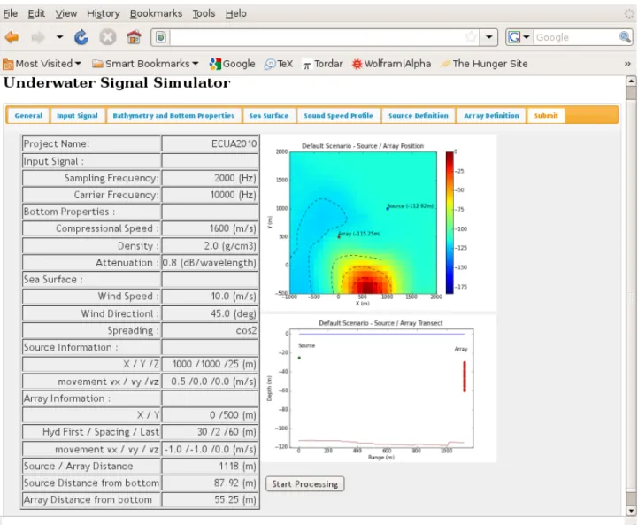
The user interface permits the configuration of several pa-rameters to perform a simulation. After a user’s login a pre-defined configuration is presented, each in a separate tab, containing bathymetry, input signal, sea surface, sound speed profile, source and receiver geometry and velocities (see Fig.1); the user’s e-mail is preserved for later updates regarding the state of the simulation. The simulation sce-nario can be viewed at the last tab (see Fig.2); by clicking a submit button the simulation is queued and launched for processing. The simulator does not allow to submit a job if the information has been entered incorrectly (for instance if the source or the hydrophones are above the sea surface or below the sea bottom), or if data has been incorrectly formatted (for instance by typing a character in a field re-questing a decimal value). The final submit page presents a source/receiver geometry, showing their starting position and the surrounding bathymetry. Users may also upload dy-namically their custom bathymetry, sound speed profile and input signals. Files can be uploaded inside the web inter-face, and their graphical representation is updated automati-cally. All graphics shown in the web interface are generated on the fly by Python scripts, using the matplotlib and scipy Python modules. Those scripts are interfaced to the web server through the mod python module.
2.3
The scheduling system
Once a user submits a simulation through the web inter-face a file with the given configuration is generated using PHP code and passed to a Python script, which functions as scheduler. The scheduler dispatches the received jobs to one of the available processing nodes and sends an e-mail to the user showing the given configuration of the submitted job and informing that the processing has begun. The sched-uler remains in a sleep state waiting for the signal from the processing node to the job to be completed. The process-ing nodes are two dual-processor quad-core machines with 20GB of RAM each, located physically in a nearby network from the web server. Processing nodes can be added or re-moved dynamically by the administrator. The job is exe-cuted on the dispatched processing node using a
combina-tion of matlab code and the Bellhop[2] or TRACE3ray
trac-ing models (although the current configuration uses
Bell-3Webpage: http://www.siplab.fct.ualg.pt/models/trace/manual/index.html.
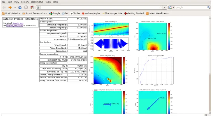
hop by default). Once the processing is complete another script is executed; it creates a series of graphical represen-tations of the simulator output, which are later presented to the user as a web page together with the calculated data. At the end of a simulation the scheduler is informed by the node that the processing is complete, it fetches the output data and sends an e-mail to the user with a web address, where the general configuration of the simulation is pre-sented and the data, stored in Matlab MAT files, can be retrieved (see Fig.3). Together with the data the user can download an M-file, which can be used to display the results in a local Matlab session. The most relevant information is displayed as figures of (transmission)time/delay, (trans-mission)time/frequency, Doppler spread/delay and Doppler spread/frequency (see Fig.4).
2.4
Modeling dynamics
The modeling dynamics of the interface evolved through several stages. It started with the modeling of source–array motion, a variable bottom bathymetry and a flat surface; later it was decided to include dynamic wind-driven sur-face waves. For such waves the Pierson-Moskowitz spec-trum was first used to generate realizations of the sea sur-face. However, since the spectrum is only valid for wind speed > 10 m/s it was noticed, after several tests, that the corresponding surfaces required finer and finer grids as wind speed decreased; the net effect of such grid refinement con-sisted in a more and more noise-like behaviour of the gen-erated surface. Therefore, it was decided later to adopt the JONSWAP spectrum, which allowed to generate realistic, noise-like free surfaces, no matter how large or small wind speed was considered to be. Generally speaking sea sur-face realizations are obtained from sea sursur-face wave spectra through the following procedure:
• Generate a matrix of white noise, same size as the full power spectrum;
• perform a 2D FFT of the white noise;
• calculate the amplitude and phase of the noise trans-form;
• multiply the noise amplitude by the full spectrum; • generate a matrix of filtered noise multiplying the noise
amplitude by cos(phase) +i sin(phase);
• perform an inverse 2D FFT of the filtered noise. The appropriate spatial sampling of the spectrum is guaran-teed by normalizing the frequency power spectrum for each value of sound velocity, and by selecting the frequency at which the amplitude of such spectrum is below a particu-lar threshold. The frequency is then converted to spatial sampling and combined with the expected maximal range, to obtain the minimal number of points that allow a proper sampling of the surface wave. To avoid memory problems
Figure 1: TV-APM interface: parameter tabs.
Figure 3: TV-APM interface: results window.
there is an upper limit to the number of points that can be used. When the required number of points is higher than the limit the surface is generated for such limit. Since the result-ing surface won’t cover the entire area of source-array mo-tion a sort of mosaic procedure is then applied, i.e. parts of the original surface are replicated in those areas not covered by the surface. The motion and dispersive-like behaviour of the sea surface is obtained by considering that it moves with
group velocity cg; temporal displacements are modeled by
changing over time the phase of the Fourier transform of the sea surface. To avoid a periodicity in wave shape the wavenumber space is perturbed with white noise before con-verting the Fourier transform back to the space domain. A simulation evolves in time steps iteractively along the specified interval of transmissions, which is defined by the user’s choice of transmitted signal. For each time step the surface shape, source/array configuration and bathymetry and surface transects are updated and an acoustic calcula-tion is performed. At each iteracalcula-tion the spreading of energy in the scattering function is calculated; if it is found to be be-low a given threshold the time steps are taken to be twice as smaller as in the previous iteration and a new iteration starts by performing an additional set of calculations. Old and new results are combined to measure again the spreading of energy, and the procedure is repeated until the spreading is found to be above the threshold.
Figure 4: TV-APM interface results (first hydrophone).
3
Interface results
The flexibility of the TV-APM interface allows to study the impact of different factors on arrival scattering, namely sur-face roughness or source–array motion. The discussion of the following sections, which is focused on the analysis of (transmission)time/delay and Doppler spread/delay figures, provides some particular examples for both factors, sepa-rately, and for both factors, combined.
3.1
Surface motion
Let us start by considering a case of short range underwater propagation, with the source located at (0,1000,60) m and a single hydrophone located at (0,1500,20) m (see Fig.5). The
wind speed and direction4 corresponds to 10 m/s and 45◦,
respectively.
Figure 5: Surface motion test: source and array positions.
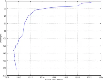
1508 1510 1512 1514 1516 1518 1520 1522 1524 0 20 40 60 80 100 120 140 160 180 200 Sound Speed (m/s) Depth (m)
Figure 6: Waveguide sound speed profile.
The averaged sound speed profile of the environment is shown in Fig.6; it exhibits a strong thermocline near 20 m, which prevents most of the acoustic energy to reach the surface be-fore being refracted back to the bottom.
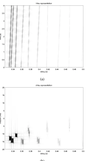
The processing takes a few seconds and produces the re-sults shown in Fig.7. The direct and single-bounce bottom paths appear as maxima with no spreads; rays with sur-face reflections suffer different spreads, due to successive reflections on surface crests and troughs, which move as the surface wave evolves in time. Micropaths fade in and
4Wind direction in the interface is taken relative to the X axis.
(a)
(b)
Figure 7: Interface results for v = 10 m/s and θ0 = 45◦
(cosine-squared spreading): (a) arrivals; (b) scattering func-tion.
out along transmissions, inducing the generation of artifacts in the scattering function, where the fading reveals itself as strips extending along all Doppler frequencies.
3.2
Source and receiver motion
Let us consider now the case of a moving source and re-ceiver. The initial configuration is the same as in the
pre-vious case, but with a flat surface and with velocities vs=
(-1,-1,0) m/s and vr= (1,1,1) m/s for the source and the
hy-drophone, respectively. Such choice of velocities is slightly unrealistic, but guarantees that the distance between the source and the hydrophone grows steadily over time. Therefore, de-lay time will increase progressively for all paths and Doppler spread can be expected to be negative for all arrivals. How-ever, since the spread depends on how many times a given
ray is being reflected on the surface and/or the bottom (see the discussion presented in [1]) it won’t be necessarily the same for different arrivals.
(a)
(b)
Figure 8: Interface results for vs= (-1,-1,0) m/s and vr =
(1,1,1) m/s (a) arrivals; (b) scattering function.
The interface results confirm the previous assumptions: the structure of arrivals is much more stable than in the previous case (compare Fig.8(a) with Fig.7(a)), but all arrivals exhibit negative Doppler spreads (compare Fig.8(b) with Fig.7(b)).
3.3
Combining surface, source and receiver
motions
The parameters used in the previous cases were combined into a common case, which was then used as input to run a simulation through the TV-APM interface. The simulation results are shown in Fig.9 and reveal how the combined ef-fects of source–array and surface motion can drastically al-ter the spread of arrivals in the scatal-tering function. If in the
(a)
(b)
Figure 9: Interface results for both surface, source and array motions: (a) arrivals; (b) scattering function.
previous case the spreads were unambiguosly distributed to-wards negative values of Doppler frequencies now only the direct and single-bottom bounced paths can be clearly seen, while other paths vanish due to arrival fading.
4
Conclusions and future work
The results obtained by the project participants are encour-aging and indicate that the current implementation of the TV-APM interface has being evolving in the correct direc-tion. Based on the experience and opinion of different users it is planned to extend the capabilities of the interface pur-suing the following goals:
• to introduce a more realistic representation of bottom features by relying on experimental data to character-ize bottom properties along different directions;
• to introduce a more realistic representation of spatial and temporal characteristics of sound speed by relying on empirical orthogonal functions;
• to improve the interface performance by learning with simulation failures, and to extend the existing code so it can avoid potentially failure configurations; • to take advantage of the multi processor capabilities
of available nodes to achieve higher rates of computa-tional speed (required for the processing of complex dynamic waveguides);
• to model additional types of source–array motion, namely random walk-like variations of position;
• to implement additional functions to allow an user to save and restore a previous simulation.
5
Acknowledgement
This work is supported by European Commission’s Seventh Framework Programme through the grant for Underwater Acoustic Network (UAN) project (contract no. 225669). It was also supported by the Portuguese Foundation for Sci-ence and Technology through the grant for PHITOM project (PTDC/EEA-TEL/71263/2006).
References
[1] Rodr´ıguez O.C., Silva A.J., Gomes J.P., and Jesus S.M. Modeling arrival scattering due to surface roughness. In Proceedings of ECUA2010, Istambul, Turkey, July 2010.
[2] Porter M. The BELLHOP Manual and Users Guide. HLS Research, La Jolla, CA, USA, 2010.