Adriana Andrade Sousa Rocha
Licenciada em Ciências de Engenharia do Ambiente
Underwater noise propagation models
and its application in renewable energy
parks: WaveRoller Case Study
Dissertação para obtenção do Grau de Mestre em Engenharia do Ambiente
Orientador: Maria Helena Costa, Professora Associada c/
Agregação, FCT-UNL
i
Underwater noise propagation models and its application in renewable energy parks: WaveRoller Case Study
Copyright Adriana Andrade Sousa Rocha, Faculdade de Ciências e Tecnologia da Universidade Nova de Lisboa (FCT/UNL).
A Faculdade de Ciências e Tecnologia e a Universidade Nova de Lisboa tem o direito, perpétuo e sem limites geográficos, de arquivar e publicar esta dissertação através de exemplares
iii
Acknowlegments
Firstly, I would like to thank my family and friends who supported me during this process. It was
them who always motivated me and didn’t let me give up.
To the friends I met in college, I could not fail to thank the support and friendship that they showed, always believing in me and my abilities throughout the course and writing of the thesis.
Special thanks to Professor Maria Helena Costa, who accepted to be as her tutor and contacted WavEC Offshore Renewables so that I could join a team and write my dissertation at their facilities.
To Teresa Simas and Erica Cruz, thank you very much. Without them I would not have been able to do this job. Erica was my companion in the simulation process, helping me with the software and never giving up even when things did not work out the way we expected. I hope to have corresponded to the trust deposited with the preparation of this dissertation.
I would also like to thank DHI for granting me the student license to work with MIKE Zero - Underwater Acoustic Simulator and for all the support and patience that the support team has shown to answer my questions about the software.
To all of you, thank you very much.
v
Abstract
In the light of global warming, large-scale transition to renewable power sources is a worldwide challenge, playing wind power a significant role. Sea wave energy is being increasingly regarded in many countries as a major and promising resource but, like all forms of energy conversion, it will inevitably have an impact on the marine environment.
WaveRoller, a Wave Energy Conversion Device, is installed in front of Almagreira beach, on the west coast of Portugal. The purpose of this thesis is to study and quantify the underwater radiated noise from this device using an underwater acoustic model in order to estimate potential effects it may have in the marine environment. The model used to run the data will be MIKE Zero – Underwater Acoustic Simulator by DHI .
In the study site only cetacean species are expected to occur. Results showed that behavioural responses might be expected for low and mid-frequency cetaceans if they swim close to the
device. Also, the device shouldn’t be installed in an area in which a population of cetaceans exists
in a 28m ray. For these individuals, injury can be assumed if SEL (Sound Exposure Level) is
higher than 215 dB re 1μPa2.s, for non-pulse sounds. Results showed the calculated maximum
SEL of the Waveroller sound is 150 dB re 1μPa2.s and therefore no injury is expected.
MIKE Zero – Underwater Acoustic Simulator is a powerful tool to test any device that produces underwater noise and offers the possibility to create Surface Sound maps of results by using MIKEXYZ Converter tool.
vii
Index
1. Introduction……….…….…1
1.1. General aspects of acoustics………...………..…...….1
1.2. Underwater noise and its effects on marine mammals…...3
1.3. Basic principles of Modeling………...………..……...………….………..6
1.4. Examples of models………...……...……….8
1.5. Aim of the thesis………...…………....……….………11
2. Case Study……….……….……….12
3. Methodology………..………..14
3.1. Data……….14
3.2. MIKE Zero –Underwater Acoustic Simulator………..………..……...16
4. Results………..………....17
5. Conclusions……….………23
ix
Index of Figures
Figure.1: Relationship between temperature and sound speed in Deep Ocean………..2
Figure 2: Table showing different models and its advantages and disadvantages……..……….11
Figure 3: WaveRoller in operation (Source: AW-Energy)……….………...13
Figure 4: Surge Phenomenon (Source: AW-Energy)……….…….…….14
Figure.5: Georeferenced Case Study Area: Bathymetry data and shoreline using QGIS………15
Figure.6: Workspace after triangulation, using MIKE Zero UAS………...……....16
Figure.7: Workspace in Mesh file format using MIKE Zero UAS………..…17
Figure 8: Sound Exposure Level spectrum for WaveRoller along a 500 m transect……….…..18 Figure 9: Sound Exposure Level spectrum for WaveRoller………...…19
Figure 10: Sound Exposure Level for WaveRoller at frequency = 200 Hz…………..…….…..19
Figure 11: Sound Exposure Lever for WaveRoller at frequency = 160 Hz………..…..21
xi
Abbreviations and acronyms
UAS – Underwater Acoustic Simulator DHI – Danish Hydrological Institute SEL – Sound Exposure Level TL – Transmission Loss
TTS – Temporary Threshold Shift PTS – Permanent threshold Shift GPS – Global Positioning System
QGIS – Quantum Geographic Information System
UTM – Universal Transverse Mercator dB – Decibels
Hz – hertz kHz - kilohertz
CCDR-LVT – Comissão de Coordenação e Desenvolvimento Regional de Lisboa e Vale do
Tejo
1
1.
Introduction
1.1.
General aspects of acoustics
Sound consists of a regular motion of the molecules of an elastic substance. Because the material is elastic, a motion of the particles of the material, such as the motion initiated by a sound projector, communicates to adjacent particles creating a sound wave outward from the source at a velocity equals to velocity of sound (Urick, 1983). Sound propagation is not the same as in the air when the propagation channel is the ocean. The main importance of sound within the ocean resides in the fact that the ocean is transparent to acoustic waves, while practically opaque to electromagnetic radiations (Erbe and Farmer, 2000). It seems to be the only radiation that can be propagated through long distances within the sea, especially at lower frequencies. Because of it, and adding the fact that the bandwidth available for communication is extremely limited, underwater acoustic channels are generally recognized as one of the most difficult communication media in use today (Stojanovic and Preisig, 2009).
The main variable affecting sound propagation in the ocean is sound speed, and is a function of three main parameterseters: depth, salinity and temperature. Sound speed increases both with temperature and pressure, then it also varies with season, diurnal changes, geographical location, and time, as these parameters affect the oceanographic conditions of the water column (affecting indirectly the three parameters mentioned before). A typical value of 1500 m/s is normally given, even though it is not homogeneously presented within the ocean (Barrio, 2009).
2
Figure.1: Relationship between temperature and sound speed in Deep Ocean. (Source: Etter, 2013)
The sea surface is both a reflector and a scatterer of sound (Urick, 1983). At calm seas the acoustic impedance at the water surface is very high. Hence, the surface would be almost totally reflecting. However, under normal conditions the rough sea surface caused by wind-driven waves induces random scattering of the reflected sound (Bolin et al., 2009). When the surface is in motion, as is
always true on the surface of the sea, it produces upper and lower sidebands in the spectrum of the reflected sound that are the duplicates of the spectrum of the surface motion. Thus, a frequency-smearing effect is produced on a constant-frequency signal, having significance for narrow-band underwater acoustic communications (Urick, 1983).
The sea bottom is also a reflector and a scatterer. However, the reflection of sound from the seabed is more complex than from the sea surface due to variations on acoustics properties (because of the composition that can vary from hard rock to soft mud) (Urick, 1983). Also, the seabed is often layered with a density and a sound velocity that change gradually or abruptly with depth (Farcas
et al., 2015).
In travelling through the sea, an underwater sound signal becomes delayed, distorted and weakened (Urick, 1983). Transmission Loss, TL, is a standard measure for underwater acoustics of the change in signal strength with range defined as the ratio in decibels between the acoustic intensity at a field point and the intensity I0 at 1m distance from the source (Jensen et al., 1994).
The Intensity of the wave can be explained as a certain amount of energy per second across a unit area oriented normal to the direction of propagation (Urick, 1983). Equation 1 shows the relation between Transmission Loss and the Intensity of the wave.
𝑇𝐿 = 10 𝑙𝑜𝑔 (I0/I1) [dB] (Eq.1)
Transmission Loss is due to the sum of two major processes: Spreading and Attenuation (which includes Absortion and Scattering losses).
3
equally in all directions so as to be equally distributed over the surface of a sphere surrounding
the source, it’s applied nearfield, and being r1 and r2 two different ranges (r2 > r1), Transmission
Loss is given by
𝑇𝐿 = 10 𝑙𝑜𝑔 (I1/I2) = 20 𝑙𝑜𝑔 r2 [dB] (Eq.2)
When the medium has plane-parallel upper and lower bounds and sound cannot cross them, Cylindrical spreading take place. It happens at moderate and long ranges whenever sound is trapped by a sound channel in the sea (Urick, 19839). This regions of low sound speed are known as the Deep Sound Channel, whose axis is at the sound speed minimum (Jensen et al., 1994). In
this case, and having once again two different ranges, r1 and r2, Transmission Loss is given by
𝑇𝐿 = 10 𝑙𝑜𝑔 r2 [db] (Eq.3)
On the other hand, Attenuation loss varies linearly with range and it’s expressed by a certain
number of decibels per unit of distance (Urick, 1983). An important property is the fact that it increases with signal frequency due to the transfer of acoustic energy into heat (Absortion).
The effects of sound reflection at the surface, bottom and any objects, and sound refraction in the water leads to a Multipath Propagation phenomenon. When a source launches a beam or rays, each one will follow a different path, and a receiver placed at some distances will observe multiple signal arrivals. Propagation paths and their strengths and delays are determined by the geometry of the channels and its reflection and refraction properties, so a ray travelling over a longer path may do so at a higher speed, thus reaching the receiver before a direct stronger ray (Stojanovic and Preisig, 2009). These phenomena cause fluctuations in phase and amplitude at a signal receiver, signal distortion, decorrelation of signal between separated receivers, and frequency
broadening (Urick, 1983). Time variability is also an important factor. Channel’s time variability
can be caused by inherent changes in the propagation medium or changes that occur because of the transmitter/receiver motion. The first case can occur in very long timescales such as monthly
changes on water’s temperature and does not affect the instantaneous communication level, or in
short timescales and affect the signal. An example of this happens when surface waves cause the
displacement of the reflection point and, as a result, the signal suffers scattering and there’s a
spread of the Doppler Effect (Stojanovic and Preisig, 2009).
By so, sound propagation in the water column is characterized by three major factors: Attenuation, Time-varying Multipath Propagation, and low speed of sound (Farcas et al., 2015).
1.2. Underwater noise and its effects on marine mammals
In the light of global warming, large-scale transition to renewable power sources is a worldwide challenge, playing wind power a significant role (Bolin et al., 2009). This demand for renewable
energy has led to construction of offshore wind farms with high-power turbines, and many more
wind farms are being planned for the shallow waters of the world’s marine habitats (Madsen et al., 2006) and have raised concerns over impacts of underwater noise on marine species (Bailey et al., 2010). On the other hand, sea wave energy is also being increasingly regarded in many
countries as a major and promising resource.
4
and various mammals, which always exist in the background of the sea. Localized noise is only present in certain areas (Huang, 2015). Noise is known to affect marine mammals in a variety of ways and under certain circumstances can be damaging (Erbe and Farmer, 2000). Vibration produced by offshore wind turbines during their normal operation transmits through the tower into the foundation where it interacts with the surrounding water and is released as noise (Marmot,
et al., 2013).
Noise from wind turbines comes in two forms: the first is aerodynamic noise from the blades slicing through the air leading to the characteristic swish-swish noise; the second is mechanical noise associated with machinery housed in the nacelle of the turbine. Aerodynamic noise travels through the surrounding air to the interface between the air and water where it’s almost entirely
reflected due to the large impedance contrast between air and water. Little aerodynamic noise enters the marine environment. Conversely, the mechanical noise has a strong structural pathway between the drive train (where the vibration is created), through the nacelle support frame, tower, into the foundation and finally from the foundation into the surrounding water where it is released as noise. The great majority of noise in the marine environment due to wind turbines is therefore related to mechanical vibration in the drive train. These vibrations are created by imbalances of the rotating components, the teeth in the gearbox coming into contact with each other (referred to as gear meshing), and electro-magnetic interaction between the spinning poles and stationary stators in the generator. Each of these vibration sources occurs in discrete frequency bands related to the rotation speed of each component: the vibrations therefore tend to be tonal (as opposed to broad band). Rotational imbalances tend to occur at very low frequencies (< 50 Hz), while gear meshing and electro-magnetic interactions tend to occur at low to moderate frequencies (50 Hz to 2 kHz).
The amplitude of the vibration of a wind turbine and related noise emitted by the foundation is controlled by the size of the excitation force, the frequency of structural resonances and the level of damping in the structure. The magnitude of the excitation of the drive train is related to the torque acting on the rotor, which is dependent on the wind speed. The amplitude of vibration of the turbine increases with the square of wind speed at the hub height. It is likely, therefore, that the noise emitted by the foundation will also rise with wind speed.
Mechanical noise can also be amplified by structural resonances within the wind turbine. Structural resonances are the harmonic frequencies at which a structure vibrates when excited by a discrete event, such as the frequency a bell rings when struck. Yet, all structures contain some level of internal damping. Damping is the dissipation of vibration energy via processes like heat loss and has the effect of reducing the amplitude of vibration. In general, steel structures such as jackets have less damping than structures built from granular materials such as concrete foundations. The level of internal damping will therefore affect the noise emitted by different types of foundations.
At the interface between the foundation and water, the vibration of the foundation oscillates water molecules to produce a pressure wave which radiates away from the foundation as sound (Marmo
et al., 2013). As the sound propagates away from the foundation its intensity is reduced with
distance due to geometric spreading and absorption. Water absorbs high frequency sound more quickly than low frequencies; low frequency sound therefore propagates further (Stojanovic and Preisig, 2009).
5
lower frequency cut off as sound can only propagate if the wavelength is less than or equal to 4 times the water depth (Urick, 1983).
Regarding wave power, the main disadvantage, as with the wind from which is originates, is its (largely random) variability in several time-scales: from wave to wave, with sea state, and from month to month (although patterns of seasonal variation can be recognized). The wave energy absorption is a hydrodynamic process of considerable theoretical difficulty, in which relatively complex diffraction and radiation wave phenomena take place (Falcão, 2010).
The wave energy level is usually expressed as power per unit length (along the wave crest or
along the shoreline direction); typical values for ‘‘good’’ offshore locations (annual average) range between 20 and 70 kW/m and occur mostly in moderate to high latitudes. Seasonal variations are in general considerably larger in the northern than in the southern hemisphere (Cruz, 2008, quoted by Falcão, 2010) which makes the southern coasts of South America, Africa and Australia particularly attractive for wave energy exploitation (Falcão, 2010). The conversion of wave energy into electrical energy has the potential to become a clean and sustainable form of renewable energy conversion. However, like all forms of energy conversion it will inevitably have an impact on the marine environment, although not in the form of emissions of hazardous substances (gases, oils or chemicals associated with anticorrosion). Possible environmental issues associated with wave energy conversion include electromagnetic fields, alteration of sedimentation and hydrologic regimes and underwater radiated noise (Haikonen, 2014).
There are different types of wave energy conversion devices: Point Absorbers, Attenuators, Terminators (or Oscillating Water Collumn), Oscillating Wave Surge Converters and Overtopping Devices.
Point Absorbers use a mechanism consisting in one immobile component and another that follows the wave motion. The potential noise associated with the operation of this device would likely be continuous and may contain tonal features with most of the sound energy at frequencies less than a few kilohertz; Attenuators consist of long multi-segmented floating structures oriented parallel to the wave travel direction; Terminators are positioned perpendicular to the wave motion and are typically installed on near shore. The noise associated to their operation is the noise from the air expelled through the turbine that is generated in air but can couple also into the water. Oscillating Wave Surge Converters work as a pendulum responding to wave surges. The back and forth movement of water driven by wave surge puts the composite panel into motion; finally, Overtopping Devices consist of elevated reservoirs that are filled by waves spilling over a ramp and empty back into the ocean below through a drain creating a head pressure across the outlet that forces water through hydro turbines (JASCO, 2009).
Depending on the distance between source and receiver, four zones of noise influences can be defined (Richardson et al., 1995). The zone of audibility is defined as the area within which the
animal is able to detect the sound. It is limited by two factors: by the critical band levels falling
6
level is high enough to cause tissue damage resulting in either temporary threshold shift (TTS) or permanent threshold shift (PTS) or even more severe damage (Richardson et al., 1995; Erbe and
Farmer, 2000). Threshold shift depends on factors such as the spectral characteristics of the noise (frequency and amplitude), the amount of energy per time for impulsive noise, the hearing sensitivity of the subject, the duration of noise exposure and the duty cycle, or recovery time between exposures (Erbe and Farmer, 2000).
Marine mammals are also indirectly affected by noise in the case that noise reduces the availability of prey. For example, noise-induced effects in fish include swim bladder resonance, blast injury of fish, larvae and eggs, a decrease in reproductivity, and possible habitat avoidance (Erbe and Farmer, 2000). Hence, noise disturbance can have a role in causing long-term displacement or abandonment of a part of the range due to changes on food abundance (Richardson et al., 1995).
Regarding long-term effects, there is most evidence that most types of disturbance do not cause mortality (Richardson et al., 1995).
1.3.
Basic Principles of Modeling
As said previously, many organisms depend on sound for communication, predator/prey detection and navigation. The acoustic environment can therefore play an important role in ecosystem dynamics and evolution. A growing number of studies are documenting acoustic habitats and their
influences on animal development, behaviour, physiology and spatial ecology, which has led to
increasing demand for passive acoustic monitoring expertise in the life sciences (Merchant et al.,
2015).
Modeling acoustic propagation conditions is an important issue in underwater acoustics and there exist several mathematical/numerical models based on different approaches. Some of the most used approaches are based on Ray Theory (by solving the wave equation), modal expansion and wave number integration techniques (Hovem, 2013).
Ray Theory is restricted to high frequencies or short wavelengths and the results and conclusions therefrom are called ray acoustics (Urick, 1983). Ray acoustics is based on the assumption that sound propagates along rays that are normal to wave fronts, the surfaces of constant phase of the acoustic waves. When generated from a point source in a medium with constant sound speed, the wave fronts form surfaces that are concentric circles, and the sound follows straight line paths that radiate out from the sound source. If the speed of sound is not constant, the rays follow curved paths rather than straight ones. The computational technique known as ray tracing is a method used to calculate the trajectories of the ray paths of sound from the source. (Hovem, 2013).
Another theory is Normal-Mode Theory, in which the propagation is described in terms of
characteristic functions called normal modes. Although it’s suitable for a sound propagation in
shallow water, comparing to ray theory, it gives little insight on the distribution of the energy of the source in space and time (Urick, 1983).
7
Most of the propagation models made until the present have been considering sound propagation in 2D. This means a limitation in shallow waters, where obliquely incident rays are reflected from
the bottom into a different vertical plane. That is called “horizontal refraction”, and requires a 3D
modelling, where the sound field is given in depth and range, but also in azimuth (Range Dependent Models) (Barrio, 2009). Five principal deterministic models can be mentioned for describing sound propagation within the sea (deterministic because they neglect the effect of fluctuations in the sound speed profile by small scale turbulences, internal waves, among others):
Ray tracing. A primary advantage of these methods is their simplicity. They depend only on ray-surface intersection calculations, which are relatively easy to implement and have computational complexity that grows sub linearly with the number of surfaces in the model. Another advantage is generality. As each ray-surface intersection is found, paths of specular reflection, diffuse reflection, diffraction, and refraction can be sampled, thereby modeling arbitrary types of indirect reverberation, even for models with curved surfaces. The primary disadvantages of path tracing methods stem from the fact that the continuous 5D space of rays is sampled by a discrete set of paths, leading to aliasing and errors in predicted room responses. Wave effects, such as diffraction and caustics, cannot be handled satisfactorily which can be a limitation for bottom interactions and low frequency propagation (Barrio, 2009). In order to minimize the likelihood of large errors, path tracing systems often generate a large number of samples, which requires a large amount of computation. Another disadvantage of path tracing is that the results are dependent on a particular receiver position, and thus these methods are not directly applicable in virtual environment applications where either the source or receiver is moving continuously (Funkhouser et al., 1998);
Normal-Mode techniques; A normal mode of an oscillating system is a pattern of motion in which all parts of the system move sinusoidally with the same frequency and with a fixed phase relation. The free motion described by the normal modes takes place at the fixed frequencies. These fixed frequencies are known as its natural frequencies or resonant frequencies. It shows advantages such as the fact that functions do not have to be calculated at all intermediate ranges between source and receiver (mode functions in deep, stable part of the water column are calculated and stored in advance, saving computation time). On the other hand, most of them do not include branch line contribution, not handling shear in the bottom (Barrio, 2009);
Multipath expansion – doesn’t have solutions for range dependence, so it won’t be considered;
Wave number Integration techniques, a method for an axisymmetric atmosphere, with
the effective sound speed accounting for wind where the ground surface is characterized by the ground impedance and the atmosphere is represented by vertical profiles of the wind velocity and the temperature. The sound field in each layer is computed in the horizontal wave domain, taking into account the appropriate continuity equations at the
interfaces between the layers. This method is also called “Fast Field Program”;
8
demand of computer time and memory (limited to relative low frequencies and unrealistically short ranges; and
Parabolic equation models. This model assumes that the speeds of energy propagation are similar to a reference speed. Unlike the ray model, the PE model handles all the
diffraction effects in the acoustic channel. Therefore, it is more suitable to lower
frequencies than the ray model (Huang, 2015). In underwater acoustics, the primary motivation for these equations has been the need to predict sound propagation in ocean environments with significant horizontal variation (e.g., continental slopes, ocean fronts, and eddies). These equations can treat such complicated environments in a relatively simple way because it neglects backscattered waves and uses a "marching" algorithm to propagate waves outward from the source. Given a starting solution at the source, the PE advances the solution in range, taking into account horizontal changes in the environment as the solution is stepped out (Gilbert et al.,1989). Despite this, there’s a lack of precision in this method and it’s impractical in high frequency regimes, as run time increases
rapidly with higher frequency (Barrio, 2009).
1.4.
Examples of models
In order to compare different models, examples for each type of model regarding the development of the wave equation are presented:
Ray Theory
There have been a number of efforts to modify conventional ray theory in order to develop improved methods that provide more accurate results but retain computational efficiency. One such method is Gaussian beam tracing. With this technique, a fan of rays is traced from a point source with trajectories governed by the standard ray equations. The Gaussian beam method associates with each ray a beam with a Gaussian intensity profile normal to the ray. An additional set of equations which govern beam width and curvature are integrated along with the standard ray equations. The Gaussian beam tracing method has been adapted to the typical ocean acoustics waveguide and has been implemented as a tool called BELLHOP. This model has rigorously been tested and results show excellent agreement with certain full wave models at high frequencies. The method is free of numerical artifacts affecting standard ray models and still retains the computational efficiency of a ray based approach (Heitsenrether and Badiey, 2004). BELLHOP is a range-dependent ray theory model that can produce ray trace, transmission loss or arrival structure results (Calnan, 2006). Also, computational complexity of BELLHOP is independent of the frequency (Ping et al., 2013).
Various files must be provided to describe the environment and the geometry of sources and receivers, such as altimetry (providing a top reflection coefficient and a top shape), bathymetry, top and bottom reflection coefficients
9
within the main environmental file. Plot programs (plotssp, plotbty, plotbrc, etc.) are provided to display each of the input files (Porter, 2011).
Regarding outputs, BELLHOP can produce a variety of files depending on the options selected within the main environmental file. These include transmission loss, eigenrays, arrivals, and received time-series. It allows for range-dependence in the top and bottom boundaries (altimetry and bathymetry), as well as in the sound speed profile. BELLHOP is implemented in Fortran, Matlab, and Python and used on multiple platforms (Mac, Windows, and Linux) being suitable for ideal sea conditions and short ranges (Error < 10 dB).
Another model based on ray theory is SAM. Since the sound rays do not propagate in straight lines, the amplitudes, phases and arrival times of rays will vary in different ocean environments. Moreover, the actual length of the sound trajectory between a pair of transceivers is not equal to the Euclidean distance. Empirical computation does not take this into account but SAM will incorporate this stratification effect on predicting the transmission loss. Its develop is based on three steps: Initial geometrical ray tracing using a discrete set of rays to map out the sound field; Determining the eigenrays, which are defined as rays connecting the source node and the destination node, and calculating the amplitude and phase for each eigenray taking the bounces on the boundaries into consideration; and Computing the transmission loss (Ping et al., 2013).
SAM uses geometrical ray tracing and makes use of the small scale fading (here, the small scale fading is the rapid fluctuations of the amplitude and phase of a micro-path acoustic signal when
interacted with the sea medium’s boundaries (either the sea surface or the sea bottom) over a short
period of time) to predict the large-scale transmission loss. In addition, like with BELLHOP, the computational complexity of SAM is independent of the frequency while the computational complexity of other acoustic models increases quickly with the carrier frequency (ONR Ocean Acoustics Library).
Summing up, SAM program holds includes input parameters as sound speed profile, depth of the sea, locations of the source and destination, average wind speed, sea floor characteristics (density of the sea bottom sediment and bathymetry). The output is to calculate Transmission Loss of the underwater channel. SAM has a good accuracy with an error of less than 5 dB).
Normal mode techniques
One model based on normal mode techniques is KRAKEN. It provides a large number of extensions and options whose presence is an advantage to a sophisticated user and a disadvantage to the uninitiated, making it more suitable for experienced modelers and for those requiring 3D capability (Porter, 2011). KRAKEN actually consists of three different models KRAKEN, KRAKENC and KRAKEL. KRAKENC and KRAKEL are for more sophisticated users with special requirements (Porter, 1992).
KRAKEN program solves for the modes and writes them to disk. Elastic media are allowed but material attenuation in an elastic medium is ignored. The inputs include the type of top boundary condition, attenuation, reflection coefficient, roughness of the interface, sound speed profile, the number of source and receiver depths, and source and receiver locations (Porter, 1992).
Another program is Program MOATL. This program, regarding a range-dependent environment case, runs a 3-layersolid basement and speed profile depends on depth.
10
the density of the sediment layer to that of water and ration of the density of the basement to that of water (Miller and Wolf, 1980).
Finite element methods
There are few models based on finite element methods. Actually, most of them are updates of previous models. One of them is RDOAST – OASES Range-dependent Transmission Loss Module and comes from the OASES model. It uses a Virtual Source Approach for coupling the
field between range-independent sectors, basically using a vertical source/receiver array, and a single-scatter, local plane wave handling of vertical discontinuities (Schmidt, 2011).
Input parameters cover number of frequencies, density, roughness, compressional attenuation and depth of the layers, number or sources, source depths and number of receivers and their depth.
Parabolic equations
At last, based on the parabolic equation method we have HAMMER. This method is often applied to predict the range-dependent sound levels over a single transect in two-dimensions away from the sound source and HAMMER extends this methodology to apply the parabolic equation method over a number of radials, giving three dimensional coverage over the model area. HAMMER was designed to predict the response of marine species to underwater sound and combines a 3-dimensional range-dependent sound propagation model with data from a hydrodynamic model which in turns supplies data to an ecological response for target species. (Rossington et al., 2013). The model takes into account bathymetry and sound attenuation, as well
as changes in the sound speed with depth. All simulated species are then studied in terms of their noise avoidance (with parameters as direction and speed).
Another model that has been developed and enhanced in recent years to become a fully modern underwater acoustic propagation modelling tool capable of computing acoustic predictions in
realistic oceanic environments is PECan (Canadian Parabolic Equation model). In PECan, it’s
assumed that all environmental parameters (sound speed, density, absorption) vary linearly with
depth between points on a given coarse profile. Moreover, between coarse profiles, each
parameters varies linearly between depth points that have the same depth index which implies that common features between coarse profiles share the same depth index (Book et al., 2000).
11
Figure 2: Table showing different models and its advantages and disadvantages (Source: Urick, 1983)
Lastly there’s MIKE Zero – Underwater Acoustic Simulator (UAS), an underwater acoustic model focused on the noise propagation in the far-field with the aim of conducting a risk assessment of environmental noise impacts, developed by DHI - Danish Hydrological Institute. It belongs to a range of software products to analyze, model and simulate any type of challenge in water environments (MIKE by DHI, 2016) and it’s based on the parabolic equation method.
12
The output is given by plots of transmission loss. These results can either create plots of the 2D transect (grid plot) or 1D profiles (profile plot). Transmission loss should increase throughout the domain. The 2D transect file may include transmission loss, sound exposure level (SEL) for each frequency and for the whole spectrum, and values in the seabed. The 1D transect file may include minimum TL over depth for each frequency and overall, maximum SEL is over depth for each frequency and over all, and the depth of the minimum TL over depth and overall (DHI, 2016).
It is important to mention that effects of underwater ambient noise and masking are not addressed in UAS. For the most energetic part of the noise source frequencies of concern in most
Environmental Impact Assessment, the ambient level is approximately 100 dB lower, hence it’s
judged to have insignificantly small impact on the calculated results.
That said, this model was chosen to be tested in this case study since it is relatively new and gives the entire data for the whole water column.
1.5.
Aim of the thesis
The purpose of this thesis is to study and quantify the underwater radiated noise from an operating Wave Energy Converter using an underwater acoustic model in order to estimate potential effects it may have in the marine environment. The model used to run the data was MIKE Zero –
13
2.
Case Study
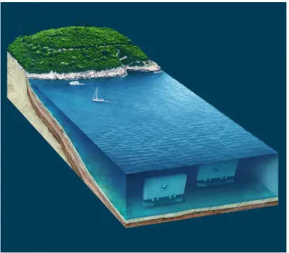
The case study concerns noise emitted by WaveRoller, a Wave Energy Conversion Device installed in front of Almagreira beach, on the west coast of Portugal, in the municipality of Peniche. The project consists of occupying an area of 860 m², of which 756 m² are part of the maritime public water domain (CCDR-LVT, 2011).
WaveRoller is an Oscillating wave surge device. It operates in near-shore areas (approximately 0.3-2 km from the shore) at depths of between 8 and 20 m. Figure 3 shows WaveRoller in operation during high tide. Depending on tidal conditions it is mostly or fully submerged and anchored to the seabed.
Figure 3: WaveRoller in operation (Source: AW-Energy)
As the WaveRoller panel moves and absorbs the energy from ocean waves, the hydraulic piston pumps attached to the panel pump the hydraulic fluids inside a closed hydraulic circuit. All the elements of the hydraulic circuit are enclosed inside a hermetic structure inside the device and are not exposed to the marine environment. Consequently, there is no risk of leakage into the ocean. The high-pressure fluids are fed into a hydraulic motor that drives an electricity generator. The electrical output from this renewable wave energy power plant is then connected to the electric grid via a subsea cable.
14
Figure 4: Surge Phenomenon (Source: AW-Energy)
As the waves approach the shore, they start "shoaling" as some of the water particles moving in a circular motion come into contact with the sea bed. This interaction with the sea bed elongates the circular motion into a horizontally elliptic shape as the particles flatten and stretch. This in turn amplifies the horizontal movement of the water particles in the near-shore area, creating a strong surge zone which is the optimal location for WaveRoller.
15
3.
Methodology
3.1. Data
The underwater noise measurements took place during the 3rd (start at 11am) and 4th of September
2014 (ended at 3pm), near the WaveRoller device.
The process consisted in scheduled measurements to characterize the source of noise (WaveRoller) and measurements along transects to assess the noise propagation. The underwater noise was recorded by using two autonomous hydrophones. Information about wave height and period was provided by the AW Energy and indicative information on wind speed was obtained from archived data available in the Windguru website. Current, water temperature and depth data were collected through CTD casts using a Valeport Limited© miniCTD to measure water temperature and salinity profile variation during the campaign. A GPS (model Garmin GPS map 60 GPCSx) was used to mark the position where measurements were carried out (Cruz and Simas, 2014).
In order to define the area, a georeferenced military map was used along with a bathymetry grid given by Instituto Hidrográfico, an organ of the Portuguese Navy, using QGIS software. The area is limited by the following coordinates: North: along the shoreline or 38,491174; South: 38,407258; East: -8,912415; and West: -9,244717. The projection used was UTM29. Figure 5 shows the workspace using QGIS.
16
Once this was done, the mesh could be established. By importing the georeferenced military map, the bathymetry grid (shape file) and the shoreline (xyz file) into MIKE Zero, and defining the workspace, it is possible to define land boundaries and form a closed domain that can be triangulated. The node points and arcs on the open boundaries must be defined by a unique integer value and these attributes are used for the model to distinguish between the different boundary types in the mesh: attributes equal to 2 and above correspond to open boundaries, attribute equals to 1 correspond to land/water boundary This task was made by using the Mesh Boundary Definition toolbar.
The next step is to triangulate the mesh. To do that, a maximum number of nodes is defined as 100000 and 26 degrees as the smallest allowable angle. Then, scatter data must be imported (bathymetry mesh and acoustic data measured in Almagreira beach. The resulting workspace with the imported shoreline and bathymetry data is shown in Figure 6, and the result exported into a mesh file is shown in Figure 7.
17
Figure.7: Workspace in Mesh file format using MIKE Zero UAS
3.2. MIKE Zero
–
Underwater Acoustic Simulator
18
4.
Results
Due to problems regarding the software, it was not possible to complete the study with information from the Almagreira beach in Peniche. That said, the simulation was performed with data from a fictitious wind farm installation in the Baltic Sea (which data already exists in the software). That is, it was assumed that the WaveRoller device was installed in the Baltic Windfarm.
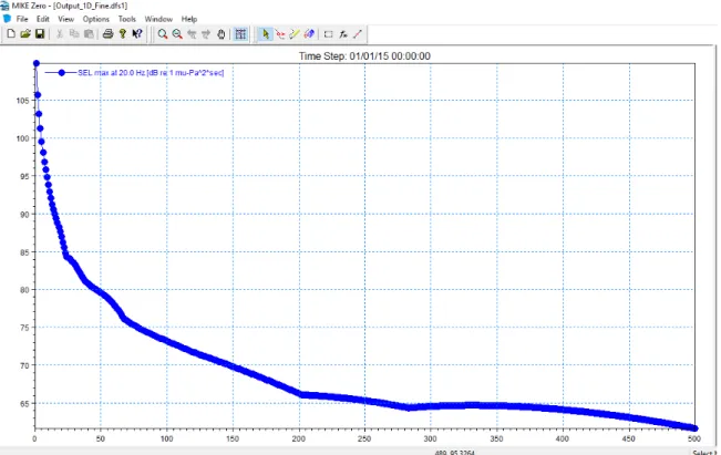
After starting the simulation, for each output both a 1D and 2D transect output are created. The 2D transect file is a dfs2 file and includes sound exposure level (SEL) for each frequency and for the whole spectrum (overall). Further the 2D transect file may include or exclude values in the seabed. The 1D transect file is a dfs1 file and includes maximum SEL over depth for each frequency and overall and the depth of the minimum TL over depth overall. Figure 8 shows the behavior of SEL along a 500 m transect, Figure 9 shows the overall SEL, and Figure 10 shows SEL for a frequency of 200 Hz.
19
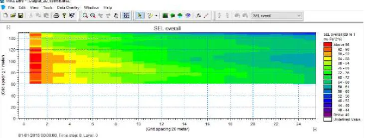
Figure 9: Sound Exposure Level spectrum for WaveRoller
20
5.
Discussion
Because WaveRoller was assumed to be installed in the Baltic Sea, this paper does not illustrate what is happening in Peniche but it can work as a test for MIKE Zero. According to Erbe and Farmer (2000) in the case of baleen whales, who are more sensitive at lower frequencies, the ray propagation model should be replaced by a model more appropriate at low frequencies such as a parabolic equation model which is the case. Also, studies using other models based on parabolic equation may be compared. Like MIKE, HAMMER takes into account bathymetry and sound attenuation by sediment, as well as changes in sound speed with depth, showing that it is the best method to simulate long range effects (Rossington et al., 2013).
All the information regarding the sound source refer to WaveRoller (as it is shown in Chapter 3
–Methodology) and MIKE’s operation was carried out in order to create the needed documents
to simulate it in Peniche (Bathymetry data and transects to establish the domain). Therefore, by using the Baltic windfarm data, the domain changed. That said, the domain for Almagreira beach is created and ready to be used. For future work and further investigations, MIKE is able to read the information and simulate sound propagation for this area.
The noise emitted by the WaveRoller is much below the noise emitted by other marine activities, including pile driving which is one of the nosiest activities that may be carried out during marine renewable energy construction, especially offshore wind projects. However, the WaveRoller noise range is similar to the noise emitted by fixed offshore wind turbines (Cruz and Simas, 2014).
Taking into account the given output for WaveRoller in the Baltic sea, some considerations can be made: By observing Figure 8, it is possible to understand that SEL decreases with range. This makes sense since sound in water suffers Spreading and Attenuation (as explained previously).
Moreover, the scale is not coherent. In the graph it’s not clear that exists SEL values for depths
from 0 m to 150 m, looking like there’s a grid spacing of 5 m. In fact, the graph shows SEL values
until a depth of 109,86 m and so the overall impression is that SEL hits its maximum at this depth.
Figures 8 and 9 show the 2D Output given by the software and it’s notorious how there’s no data
regarding SEL from 200 Hz to 500 Hz. In fact, as shown in Figure 10, SEL is showed as being constant all over the transect, and bellow 20 m of depth the data expires. On the other hand, it’s
also possible to see that from 200 Hz to 500 Hz, SEL is always between 0,00 and 0,08 dB re
μPa2.s
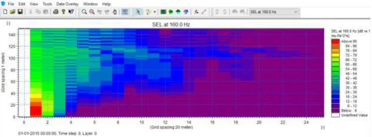
The next Figure (Figure 11) shows the SEL behavior for a frequency equals to 160 Hz. This is the last frequency that contains all the data from the sound source to the seabed.
By switching between overall SEL and SEL at different frequencies (for example 20 Hz, 40 Hz
and so on) it’s notorious that low frequency signals are absorbed less rapidly in the ocean than
high frequency signals and can therefore travel longer distances and still be detected.
Observing the graph (Figure 9) is also possible to understand that the device shouldn’t be installed
in an area in which a population of cetaceans exists in a 28 m ray. In terms of water column,
21
Figure 11: Sound Exposure Lever for WaveRoller at frequency = 160 Hz
As said previously, by the time frequencies of 200 Hz and more are chosen, the information disappears. This might be an error caused after the simulation and after running MIKE Zero UAS,
for there’s no reason for SEL being constant in these areas. On the other hand, it would be predictable for the SEL overall graph to show a green area from 200 Hz to 50 Hz and that does not happen, the information disappears. That said, the matter regarding Figure 7 and its SEL values until 109,86 m may have to do with this lack of SEL information.
The sound emitted by WaveRoller is dominant in the 125 Hz frequency band (Cruz, E. and Simas, T., 2014) and SEL values are higher for that frequency than for any other (Figure 11).
22
Despite all this, the main issue is that it is not clear how the software shows the SEL for each frequency based on a range of frequencies initially stipulated. Indeed, all the data is in a table that can be traversed in the software and SEL values are given for each meter of range and depth (1 m, 2 m, and so on). That is, it is not possible to calculate an exact distance for the actuation of a given SEL which would be interesting and more accurate.
Also, this kind of sound propagation model gives powerful information for describing geographical sound behavior and that would be the most important output for this study. Actually, there is a tool in the MIKE Zero UAS software that allows the creation of maps that translate sound information in a spatial point of view. In this way, the SEL would be visualized in the form of rays, propagating along the transect allowing the creation of maps showing potentially dangerous locations for marine fauna could be made later. Due to the lack of time this was not made for this paper.
For further work, in terms of noise impacts on marine mammals, it is important to mention that the assessment of potential impacts should take into account the auditory sensitivity of the animals. However, the fact that the study population is permanently subject to high noise levels can cause the hearing threshold to be modified (Richardson and Würsig, 1997 quoted by Cruz, 2012).
Regarding the potentially affected species, in the study site only cetacean species are expected to occur and these include baleen whales, common dolphins (Delphinus delphis), bottlenose
dolphins (Tursiops truncatus), sperm whale (Physeter macrocephalus),and harbour porpoises
(Phocoena phocoena) (Brito et al., 2008 quoted by Cruz, E., and Simas, T., 2014). The cetaceans
group is subdivided into two sub-groups: mysticetes (big cetaceans) and odontocetes. The main difference between the two suborders is that in mysticetes, the teeth are absent, being replaced by bristles of a keratinous material, with the function of filtering the water and gather food. These have different ways to use and interpret the sound and therefore they can be affected at different levels by the same sound (Cruz, E., and Simas, T., 2014). It’s important to mention that mysticetes are considered low-frequency cetacean and odontocetes is subdivided in mid and high-frequency cetaceans.
Injury is considered an elevation of the hearing threshold to a specific frequency (can be temporary – reversible, or permanent – irreversible) and sound exposure level (SEL) is currently accepted as the best metric to measure it. Injury can be assumed if SEL is higher than 215 dB re
1μPa2.s, for non-pulse sounds. By observing Figure 6, and SEL values for each frequency, the
calculated maximum SEL of the Waveroller sound is 150 dB re 1μPa2.s and therefore no
damaging injury is expected.
For low-frequency cetaceans it is assumed that the avoidance behaviour or other types of responses might occur when received levels are 120-160 dB re μPa2.s. For mid-frequency
cetaceans behavioural responses were already registered for different noise sources when received levels are around 90-120 dB re 1μPa2.s in some cases and around 120-150 dB re 1μPa2.s in other
cases. For high-frequency cetaceans behavioural responses have been already identified when
received levels are around 140 dB re 1μPa2.s in high frequency ranges (Southall et al., 2007)
23
6.
Conclusions
After finishing this work, it was notorious that Erbe and Farmer (2003) concluded that a parabolic
equation model is the most appropriate at low frequencies. It’s the case of MIKE Also, .Rossington et. al (2013) tested a parabolic equation model (HAMMER) that works with the same
input as MIKE showing that it is the best method to simulate long range effects. That said, MIKE Zero UAS is a powerful tool to test any device that produces underwater noise.
On the other hand, some weaknesses could be mentioned: It is not clear how the software shows the SEL for each frequency based on a range of frequencies initially stipulated and SEL values are given for each meter of range and depth (1 m, 2 m, and so on). That is, it is not possible to calculate an exact distance for the actuation of a given SEL. Regarding the graphs, the depth axix should have its lower value on the maximum depth and not the 0 value, for a better understanding.
24
7.
References
Austin, M., Chorney, N., Ferguson, J., Leary, D., O’Neill, C. and Sneddon, H., (2009).
Assessment of Underwater Noise Generated by Wave Energy Devices. JASCO Applied Sciences on behalf of Oregon Wave Energy Trust, Canada
AW-Enery (2016). Available on http://aw-energy.com/ (accessed on June, 6th 2016)
Bailey, H., Senior, B., Simmons, D., Rusin, J., Picken, G., and Thompson, P., (2010). Assessing underwater noise levels during pile-driving at an offshore windfarm and its potential effect on marine mammals.
Barrio, A.O., (2009). Modelling underwater acoustic noise as a tool for coastal management. Dissertação de Mestrado em Gestão da Água e da Costa (Curso Europeu), Faculdade de Ciências e Tecnologia da Universidade do Algarve, Faro.
Blastein, I.M., (1974). Comparisons of Normal Mode Theory, Ray Theory, and Modified Ray Theory for arbitrary sound velocity profiles resulting in convergence zones. Naval Ordnance Laboratory White Oak, Maryland
Bolin, K., Boué, M., and Karasalo, I., (2009). Long range sound propagation over a sea surface. Acoustical Society of America, p. 2191-2197
Brooke, G.H., Ebbeson G.R. and Thomson, D.J., (2000). PECan: A Canadian Parabolic Equation Model for Underwater Sound Propagation. Journal of Computational Acoustics, 9, p. 69-100
Calnan, C., (2006). DMOS – Bellhop Extension. Defense Research and Development Canada –
Atlantic, Canada
CCDR-LVT (2011). Study Environmental Incidences No 57/2011 "WaveRoller Peniche". Coordination and Regional Development Commission of Lisbon and Tagus Valley. Portugal
Cruz, E., and Simas, T., (2014). Environmental monitoring and management of the WaveRoller project Peniche: Underwater noise monitoring report. WavEC – Offshore Renewables, Lisbon.
Dhatt, G., Touzot, G., and Lefrançois, E., (2012). Finite Element Method, ISTE, London
Erbe, C. and Farmer, D., (2000). A software model to estimate zones of impact on marine mammals around anthropogenic noise. Institute of Ocean Science, p. 1327-1331
Etter, P., C., (2013). Underwater Acoustic Modelling and Simulation. Spon Press/Taylor&Francis, 3rd edition. New York, USA
Falcão, A.O (2010). Wave energy utilization: A review of the technologies. IDMEC, Instituto Superior Técnico, Technical University of Lisbon, Lisbon, Portugal
25
Gilbert, K.E. and White, M.J., (1989). Application of the parabolic equation to sound propagation in a refracting atmosphere. Acoustical Society of America
Haikonen, K., (2014). Underwater radiated noise from Point Absorbing Wave Energy Converters: Noise Characteristics and Possible Environmental Effect. Dissertation from the Faculty of Science and Technology, Uppsala, Sweden.
Heisenrether, R.M. and Badiey, M., (2004). Modelling Acoustic Signal Fluctuations Induced by Sea Surface Roughness. Ocean Acoustic Laboratory, Newark.
Hovem, J.M., (2013). Modeling and Measurement Methods for Acoustic Waves and for Acoustic Microdevices. Chapter 23: Ray Trace Modeling of Underwater Sound Propagation, p. 573-596
Huang, J., (2015). Simulation and Modeling of Underwater Acoustic Communication Channels with Wide Band Attenuation and Ambient Noise. Thesis for the degree of Master of Science. School of Computer Science at Carleton University. Ontario
Jensen, F., Kuperman, W., Porter, M., Schmidt, J., (1994). Computational Ocean Acoustics. American Institute of Physics, New Cork.
Kebkal, K.G., Bannasch, R., (2002). Sweep-spread carrier for underwater communication over acoustic channels with strong mulyipath propagation. Acoustical Society of America
Madsen, P.T., Wahlberg, M., Tougaard, J., Lucke, K. and Tyack, P., (2006). Wind turbine underwater noise and marine mammals: implications of current knowledge and data needs. Marine Ecology Progress Series, Vol. 309: p.279-295
Marmo, B., Roberts, I., Buckingham, M.P., King, S. and Booth, C., (2013). Modelling of Noise Effects of Operational Offshore Wind Turbines including noise transmission through various foundation types. Edinburgh: Scottish Government
MIKE (2016). Underwater Acoustic Simulator: User’s guide. DHI
MIKE by DHI (2016). Consulting the website https://www.mikepoweredbydhi.com/ on June, 18th
2016.
Miller, J.F. and Wolf, S.N., (1980). Modal Acoustic Transmission Loss (MOATL): A Transmission Loss Computer Program using a Normal-Mode Model of the acoustic field in the Ocean. Naval research Laboratory. Washington D.C.
Norrie, D.H. and de Vries, G., (1973) The Finite Element Methods, Fundamentals and Applications. Academic Press Inc., USA
ONR Ocean Acoustics Library. Available online: http://oalib.hlsresearch.com/ (accessed on April 7th, 2016)
Porter, M.B., (1992). The KRAKEN normal mode program. Naval Research Laboratory. Washington D.C.
26
Richardson, W.J., Greene Jr., C.R., Malme, C.I. and Thomson, D.H., (1995). Marine Mammals and Noise, Academic Press, California, USA
Richardson, W.J., Greene, C.R.G. jr., Malme, C.I. and Thomson, D.H., (1995). Marine Mammals and Noise. Academic Press, San Diego.
Schmidt, H., (2011). OASES: User Guide and reference Manual. Version 3.1. Department of Ocean Engineering. Massachusetts Institute of Technology
Southall, B. L., Bowles, A. E., Ellison, W. T., Finneran, J. J., Gentry, R. L., C.R., G. J., Kastak, D., Ketten, D. R., Miller, J. H., Nachtigall, P. E., Richardson, J. W., Thomas, J. A. and Tyack, P.
L., (2007). Marine Mammal Noise Exposure Criteria. Aquatic Mammals 33:411‐521
Stojanovic, M. and Preisig, J., (2009). Underwater Acoustic Communication Channels: Propagation Models and Statistical Characterization. IEEE Communication Magazine, p. 84-89
Tiemann, C.O., Frazer, L.N. and Porter, M.B., (2004) Localization of marine mammals near Hawaii using an acoustic propagation model, Acoustical Society of America, p.2834-2843