Declaração
Nome: Nelson Manuel Almeida Gonçalves
Endereço Electrónico: [email protected] Telefone: 937528319
Bilhete de Identidade: 13220550
Título da Tese: Large Scale Privacy Preserving Bluetooth Sensing Orientador: Doutor Carlos Miguel Ferraz Baquero Moreno Co-Orientador: Doutor Rui João Peixoto José
Ano de conclusão: 2012
Designação do Mestrado: Mestrado em Engenharia Informática
É AUTORIZADA A REPRODUÇÃO INTEGRAL DESTA TESE APENAS PARA EFEITOS DE INVESTIGAÇÃO, MEDIANTE DECLARAÇÃO ESCRITA DO INTERESSADO, QUE A TAL SE COMPROMETE.
Universidade do Minho, 31 de Janeiro de 2013 Nelson Manuel Almeida Gonçalves
It suddenly struck me that that tiny pea, pretty and blue, was the Earth. I put up my thumb and shut one eye, and my thumb blotted out the planet Earth. I didn’t feel like a giant. I felt very, very small.
Acknowledgements
First, I would like to thank Professors Carlos Baquero and Rui José, for being my advisers. Their support, knowledge and availability were fundamental to the success of this work.
Also, a special thanks to Paulo Jesus and Miguel Borges, two colleagues of mine from whom I’ve sought advice and help countless times.
To my long time friends, Pedro Gomes, Tiago Oliveira and Ricardo Gonçalves for the motivation and unconditional support they have given me.
To my friends from the Distributed Systems Laboratory, Francisco Cruz, Fran-cisco Maia, Miguel Matos, Ana Nunes, João Paulo, Luís Zamith and Ricardo Vilaça. I have learned a lot from them and will never forget the interesting discussions we’ve had.
Finally, to my parents, brother and sister, for their relentless support, love and encouragement.
Resumo
Motivados pelo cada vez maior número de dispositivos móveis, os serviços ba-seados na localização estão a tornar-se cada vez mais populares. Estes serviços utilizam informação acerca da localização física dos utilizadores, normalmente para fins comerciais ou informativos. Contudo, e particularmente para cenários de larga escala, este tipo de serviços pode constituir um risco para a privacidade dos utilizadores. Informação relacionada com localização dos utilizadores pode ser utilizada de forma direta ou indireta (associada com outra informação) para revelar informação privada acerca dos mesmos, podendo até ser suficiente para revelar as suas identidades. Este facto pode levar à rejeição deste tipo de tecnologias.
Existem contudo, maneiras não triviais de guardar informação sem comprome-ter a privacidade dos utilizadores. Nesta dissertação, apresentamos dois cenários Bluetooth, onde o problema da privacidade é solucionado através do uso de técnicas de sumarização estocásticas.
No primeiro cenário, Gate Counting, o objetivo é obter contagens precisas para o número de avistamentos de dispositivos distintos, tentando em simultâneo reduzir a quantidade de informação recolhida. Para esse efeito, fazemos uma análise a várias técnicas de contagem estocásticas que não só fornecem contagens para o número de dispositivos únicos, com uma precisão adequada, como também garantias de privacidade, tudo de uma forma eficiente em termos de espaço.
Para o segundo cenário, Causality Tracking, o objetivo é estudar os padrões de mobilidade humanos, ao mesmo tempo que, também se tenta minimizar a quantidade de informação recolhida. Com este propósito, desenvolvemos os Filtros de Precedência, uma nova técnica capaz de fornecer resultados precisos sobre a
popularidade de determinados percursos/caminhos específicos, sem comprometer
iv
a privacidade individual dos utilizadores.
Com base nestes cenários, esta dissertação demonstra que as técnicas de suma-rização estocásticas são meios viáveis para a anonimização de informação baseada na localização.
Abstract
Driven by the pervasiveness of mobile devices, location based services are be-coming increasingly popular. These services use information about the physical location of users, usually with commercial or informative purposes. However, and particularly for large scale scenarios, this type of services may pose a risk to the privacy of the users. By using location information either directly or indirectly (associated with other information), it is possible to expose personal information that users wish to keep private or even to uncover their identities. This may lead to the rejection of these types of technologies.
There are however, non trivial ways to store information without compromis-ing the users’ privacy. This dissertation presents two Bluetooth scenarios where stochastic summarizing techniques are used as a solution to the privacy problem.
In the first scenario, Gate Counting, the goal is to provide accurate counting for the number of unique devices sighted while trying to minimize the amount of collected information. For that purpose, we provide an analysis of several
stochastic counting techniques that not only provide a sufficiently accurate count
for the number of unique devices, but offer privacy guarantees as well, all in a
space efficient way.
For the second scenario, Causality Tracking, the objective is to study human mobility patterns, also while minimizing the quantity of data gathered. For this purpose, we developed Precedence Filters, a new technique, which is able to provide accurate results regarding the popularity of specific routes without compromising the individual privacy of the users.
Based on these scenarios, this dissertation demonstrates that stochastic summa-rizing techniques are viable means to the anonymization of location information.
Contents
List of Figures ix
1 Introduction 1
1.1 Structure and Contributions . . . 3
2 Literature Review 5 2.1 Location Privacy in Pervasive Computing . . . 5
2.1.1 Definition of Location Privacy . . . 5
2.1.2 Related Work . . . 7
2.2 Algorithms and data structures . . . 12
2.2.1 Hash Sketches . . . 12
2.2.2 Bloom Filters . . . 16
2.2.3 Vector Clocks . . . 19
3 Collaborative Gate Counting 23 3.1 Motivation and System Model . . . 23
3.1.1 Objectives . . . 25
3.2 Criteria . . . 25
3.3 Evaluation . . . 29
3.4 Summary . . . 31
4 Causality Tracking 33 4.1 Motivation and System Model . . . 33
4.1.1 Objectives . . . 36
4.2 Precedence Filters . . . 36 vii
viii CONTENTS
4.3 Metrics and Data Sets . . . 39
4.4 Evaluation . . . 44
4.5 Summary . . . 47
5 Conclusion 49
List of Figures
2.1 Insertion of elements in a (Hyper)LogLog Sketch . . . 15
2.2 Linear Counting Sketch after the insertion of 4 elements . . . 16
2.3 Bloom Filter with k = 3, M = 21 and m = 7, containing elements {x, y, z}. Querying for the presence of element w yields a false positive. . . 17
2.4 Vector Clocks . . . 21
3.1 Different Merge Approaches . . . 27
3.2 Gate Counter Aggregation - repeated devices appear only once . . 28
3.3 Relative error of the several techniques using various upper bounds. Average of 100 runs. . . 29
3.4 Size benchmarks . . . 30
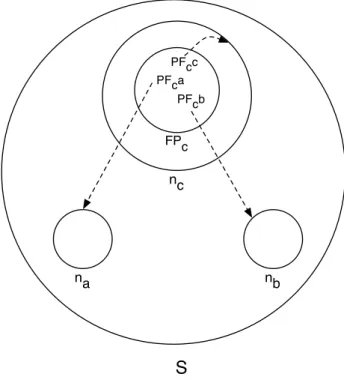
4.1 Diagram of relevant entities and data structures . . . 37
4.2 Venn diagram representation of Equation 4.1 . . . 41
4.3 Venn diagram representation of Equation 4.2 . . . 41
4.4 Number of total and distinct device sightings across the scanners . 43 4.5 Comparison between real and synthetic data set, with same param-eters . . . 44
4.6 Synthetic data sets with increasing number of devices . . . 45
4.7 Synthetic data sets with increasing trace sizes . . . 46
4.8 Synthetic data sets with increasing number of devices and trace sizes 46
1
Introduction
Propelled by the increasing usage of web enabled, context and location aware mobile devices, context aware services specially location based services (LBS) are becoming remarkably popular. The recent developments seen in technologies like GPS, GSM, Wifi and Bluetooth also worked as a catalyst in this process. Using these technologies it is possible to obtain information about the location of users. This type of information can be used both by service providers and users. Service providers can process this information to obtain a better understanding of the users behavior (e.g. by analyzing their movement) and improve their current services, as well as plans for future services and infrastructures. Users, on the other hand, can use location data to get personalized information according to their location. However, the continuous monitoring, processing and storage of location data can create privacy related problems. Location information can expose
sensitive information about users as it constitutes a quasi-identifier1according to
Bettini et al. [8].
Examples of attacks on privacy using recorded location data are not hard to find. Using a week-long database, with GPS traces of Detroit drivers whose names were replaced with pseudonyms, Hoh et al. [32] were able to determine the location of 85% of the drivers’ homes. Hightower et al.’s BeaconPrint algorithm [31] is able to
1Data that by itself does not uniquely identify a user but that in association with other information
might.
2 CHAPTER 1. INTRODUCTION accurately recognize the location of a user using only Wifi and GSM information. Researchers have also shown that, looking at the historic of someone’s location data, it is possible to predict their future whereabouts [37, 23].
While location based information is very useful, the fact that it can be used to attack the privacy of the users might be a decisive factor in the popularity and sustainability of services supported by this type of information. The solution to this problem consists in the use of privacy preserving approaches capable of ensuring both the quality of the service and the privacy of its users.
Stochastic summarizing techniques are space efficient, probabilistic
mecha-nisms, capable of producing summaries of the data they receive as input. The size of the summaries depends only on the number of input elements, not on the size of the elements. Being non-deterministic, these techniques do not allow the original
item to be recreated from its resulting summary. However they do offer a trade-of
between space and accuracy where one is obtained at the expense of the other. This dissertation aims to find if stochastic summarizing techniques are suitable as privacy preserving techniques regarding location data in large scale scenarios. As a proof of concept, we present two Bluetooth based scenarios, where we make use of these techniques to ensure the privacy of the users while trying to comply with the scenarios’ requirements.
Bluetooth technology is a relatively easy and inexpensive way to track large groups of people. Unlike technologies like GPS, Bluetooth also works well in both indoors and outdoors scenarios. This allows the tracking of individuals both inside and outside buildings allowing for more robust tracking solutions. Also, Bluetooth has a limited detection range (typically between 10 to 100 meters depending on
the number of obstacles) which makes the differentiation between nearby places
possible, thus enabling accurate tracking results. Furthermore, Bluetooth tracking is a passive tracking process, i.e, it does not require users to change their behavior. On the other hand, GPS positions are computed in the mobile device and have to be handed to the tracking entity. All these properties make Bluetooth an arguably good choice in which to base our tracking scenarios.
As Bluetooth becomes more and more pervasive, there is a growing potential
to leverage on the possibilities offered by Bluetooth scanning as a flexible
1.1. STRUCTURE AND CONTRIBUTIONS 3 and actuation in physical spaces.
Bluetooth sensing is based on a discovery process through which a device can inquire about the presence of other nearby devices. If those devices are in
discoverablemode, they will respond with their Bluetooth addresses (48 bit MAC),
and possibly additional information, such as the device name, the device type (e.g. cellphone or computer) and available services.
A Bluetooth scanner is a device that periodically scans nearby Bluetooth devices. Each time a device is detected, it registers and timestamps that event. Later, this information can be used by external services or applications. Multiple Bluetooth scanners spread all over a physical space could thus serve as collection points for Bluetooth sightings, providing a major tool for observing, recording, modeling and analyzing that space, physically, digitally and socially [46].
An infrastructure of this nature can be built from scratch given the increasingly smaller cost of the technological equipment required. Alternatively, it can be built upon the large number of Bluetooth scanners already present in some urban environments. These scanners are owned by many entities and they serve very diverse purposes, such as proximity marketing, device localization or OBEX-based interaction. They could be used, without any additional cost, as nodes in a large scale collaborative sensing infrastructure. Each node would still scan for its own purposes, but it would also share part of the generated data with a central service that would then be able to produce aggregate information of mutual interest. Both strategies make the creation of this type of infrastructure relatively simple and feasible in the short term.
The challenge, however, is how to enable this type of large scale sensing without creating an overwhelming privacy threat to the users.
1.1
Structure and Contributions
Structure
This dissertation is organized as follows: Chapter 2 presents some of the related work in the field of location privacy followed by a brief description of some
4 CHAPTER 1. INTRODUCTION describe both our Bluetooth tracking scenarios, Collaborative Gate Counting and
Causality Tracking, their requirements and the effectiveness of several stochastic
summarizing techniques in dealing with them. Chapter 5 draws some general conclusions about our work and presents some future research directions to be followed.
Contributions
As a result of the work developed in the context of this dissertation, two full papers were written. The first one [28] was published in the OTM 2011 Workshop Proceedings. The second paper [27] was published in INFORUM 2012 where it was awarded the prize for best paper in the Mobile and Ubiquitous Computing session.
Also a contribution, is the GitHub repository2with the python code for some
of the algorithms implemented during the context of this dissertation.
2
Literature Review
This chapter exposes some of the works whose content is relevant to the context of this dissertation. Section 2.1 begins by explaining the concept of location privacy in pervasive computing and it’s importance. It then follows with the presentation of some of the approaches already used in the field of pervasive computing that deal with this topic. Lastly, Section 2.2 provides some background to the algorithms and classic data structures used in our approach to ensure privacy.
2.1
Location Privacy in Pervasive Computing
As location based services become more popular and compelling, there is an increasing temptation to give away location data. However, along with this entice-ment comes an increasing concern about location privacy. Before going into any further details, it is important to correctly understand what location privacy is.
2.1.1
Definition of Location Privacy
Beresford and Stajano [7] define location privacy as:
“...the ability to prevent other parties from learning one’s current or past location.”
6 CHAPTER 2. LITERATURE REVIEW Their definition implies that a person whose location is being monitored must be able to control who has access to that information. It also acknowledges that both past and present information, regarding location, is important. While current location information might enable an attacker to find out where a person is, past
data can allow him/her to discover who the person is and where does she live/work,
and even predict future locations.
According Duckham and Kulik [15] location privacy is:
“a special type of information privacy which concerns the claim of individuals to determine for themselves when, how, and to what extent location information about them is communicated to others.”
Their definition is based upon Westin’s [52] definition of information privacy: “the claim of individuals, groups or institutions to determine for themselves when, how and to what extent information about them is communicated to others.”
Duckham and Kulik’s definition captures several aspects about location information and the way it can be shared:
• When: A user might have different concerns regarding her present and past
locations. For instance, the user may not care as much about revealing her past locations as it does about its present location.
• How: A user might be comfortable with manual location requests from her friends, however she may not want to have her friends alerted automatically when she enters a casino or a bar.
• Extent: A user might prefer to have her location reported as an ambiguous region rather than as a precise point.
These different aspects are the topic of many different computational schemes
for protecting the privacy of the users. Examples of such schemes are the use of pseudonyms instead of actual names, the deliberate addition of noise to the location data or the use of regions for location reporting instead of specific points.
2.1. LOCATION PRIVACY IN PERVASIVE COMPUTING 7
2.1.2
Related Work
In the past few years there has been an exponential increase in the number of mobile devices (smartphones, laptops, tablets). Many of these devices come equipped with several types of sensors (accelerometer , gyroscope, thermometer, GPS) as well as communication interfaces (Bluetooth, WiFi). Their pervasiveness associ-ated with their capabilities make them viable building blocks for urban pervasive infrastructures [36]. Associated with the increasing number of mobile devices is the popularity growth of Location-Based Services (LBS)[56]. LBSs determine the location of the user by using one of several technologies for determining its position, and then use the location and other information to provide personalized applications and services [55]. There are however privacy risks that stem from
the use of such services. PleaseRobMe1 was created to raise awareness for the
risks of sharing location information. Combining information from FourSquare2
and Twitter3 it demonstrates how easy it is to infer that someone is not at home.
Despite the existence of reports linking the sharing of location information with the occurrence of robberies [50, 18], there are several research works which show that most people put little value on their location privacy [1, 12, 13, 34]. How-ever, this lack of concern by the users of LBSs is usually a consequence of lack of awareness. In [34] the author notes that, despite not being worried about the privacy issues arising from location aware services, most of the users were not aware they could be located while using those services. On the other hand, the work in [13] shows that the Greeks demanded a higher price for their location data when compared with the other EU countries. According to the author, this might have been a consequence of the eavesdropping scandal involving the wiretap of Greek politicians that took place 2 months before the survey. This might indicate that people value their privacy the most when faced with consequences from the lack of it. Sharing location data at such a large scale like we see today is relatively
new. As a consequence, the effects on user privacy are not fully understood yet
[49].
According to Duckham and Kulik’s survey in [15], there are four commonly
1www.pleaserobme.com
2www.foursquare.com
8 CHAPTER 2. LITERATURE REVIEW used methods for ensuring location privacy:
• Regulatory strategies: comprised by government rules on the use of personal information.
• Privacy Policies: trust-based mechanisms established between individuals and whomever is receiving their location data.
• Anonymity: Disassociation between the individual’s personal information and individual’s actual identity. Usually obtained through the use of pseudonyms, ambiguity and cloaking.
• Obfuscation: degradation of the quality of the location data.
From these four methods, we will concentrate in the last two because they are the most relevant in the context of this dissertation.
Anonymity
The use of pseudonyms is perhaps the most obvious way to achieve anonymity. However, using same pseudonym for a long time makes it is easy for an attacker to gather enough history on an individual to infer their habits or true identity. To try to mitigate this issue, Beresford and Stajano in [7] proposed an idea which relied upon pseudonym exchange. They introduced two new concepts: mix zone and application zone. A mix zone for a group of people is defined as the maximum contiguous area where none of the group’s users exchanges information with a LBS. This prevents the users’ data from being accessed by the LBS providers. By contrast, an application zone is defined as an area where at least one of the users exchanges data with a LBS. By switching her pseudonym to a new unused one when entering a mix zone, the user ensures that there is no way for a LBS provider to distinguish between her and the other users who were in that zone. This means that there is no way for attackers to link people going into the mix zone with the ones that come out of it.
Based on a different concept, k-anonymity (introduced by Samarati and Sweeney
in [48]) Gruteser and Grunwald [29] were the first to investigate anonymity as a method to attain location privacy. According to them, a subject is considered
2.1. LOCATION PRIVACY IN PERVASIVE COMPUTING 9 to be k-anonymous with regard to location information, if and only if she is indistinguishable from at least k − 1 other subjects with respect to a set of
quasi-identifierattributes. Bigger values of k correspond to higher degrees of anonymity.
They proposed a middleware architecture and an algorithm capable of adjusting
location information resolution in spacial and/or temporal dimensions in order to
comply with a specific k-anonymity requirement. When a client requests a service,
their algorithm calculates a cloaking box/region that contains that client along with
at least k − 1 other users. That box is then used as the client’s location to request the service. If that box’s resolution is to coarse for some services, temporal cloaking can be applied by delaying the user’s service request. When more users come near the client, a smaller cloaking region can be computed. This concept has since been explored and improved in other scientific works.
Geddik and Liu’s ClickCloak algorithm [24, 25] allows each user to define her
own minimum acceptable value for k (kmin), as well as the maximum acceptable
values for temporal and spacial resolution. Furthermore, they created an efficient
message perturbation engine capable of performing location anonymization of users’ requests. This is accomplished by removing the users’ identities from the requests and with the use of spatiotemporal obfuscation of the location information.
Mokbel et al. in [44] use the k-anonymity concept as well. They presented the Casper framework which consists of two main components, a location anonymizer and a privacy-aware query processor. The location anonymizer blurs the location information about each user according to that user’s defined preferences (minimum
area Aminin which she wants to hide and minimum value for k). The query processor
tunes the functionality of traditional location-based databases to be privacy-aware. It does so by returning cloaked areas instead of exact points when queried for location information.
Unlike the previous k-anonymity based approaches that require a centralized trusted server (Anonymizer) in order to compute the cloaking regions, Ghinita et al. in [26] use a decentralized peer-to-peer approach. This fixes two issues inherent to the centralized server approach:
• Fault Tolerance - the anonymizer is a single point of failure and the system cannot work without it.
10 CHAPTER 2. LITERATURE REVIEW • Security - all requests must go through the anonymizer, so in case it becomes
compromised it would result in a serious security threat.
Their distributed protocol called PRIVÉ supports decentralized query anonymiza-tion with load balancing and fault tolerance. In PRIVÉ, for a user to be considered trustworthy and participate in the network, she needs a trust certificate obtained from a Certification Server. Users in the network trust each other and communicate using a structured peer-to-peer network. Users are grouped into clusters according to their location. Each cluster has a leader which is recursively grouped with other
leaders to form other clusters with different leaders, just like a B-Tree structure.
This allows each user to create it’s own cloaking region by using information from other nearby users. Furthermore, PRIVÉ also ensures reciprocity in the creation of cloaking regions. A cloaking region with k users satisfies reciprocity only if that same cloaking region is generated for each of users. This means that an attacker cannot use minimality attacks [54], i.e., it cannot infer which user is the source of
the request with a probability bigger than 1k.
Obfuscation
Obfuscation based techniques usually degrade the “quality” of the information in order to provide privacy protection. Even tough this may seem comparable to what
k-anonymitybased techniques do, there is a key difference: obfuscation based
tech-niques allow the actual identity of the user to be revealed (thus making it suitable
for applications that require authentication or offer some sort of personalization
[39]).
Duckam and Kulik [14] were the ones who introduced the idea of obfuscation for location privacy. They talk about three distinct types of imperfection that can be present in spacial information:
• Inaccuracy - lack of correspondence between information and reality. E.g. “Braga is in Spain”
• Imprecision - lack of specificity in the information. E.g. “Braga is in Europe” • Vagueness - special type of imprecision that concerns the existence of inde-terminate borderline cases [16]. E.g. “Braga is in western Europe”. This
2.1. LOCATION PRIVACY IN PERVASIVE COMPUTING 11 is a vague statement since there is no clear definition about the borders of western Europe.
Any of these types of imperfection can be used to obfuscate an individual’s location. In this particular case, the authors use imprecision to degrade the quality of the location information. They adopt a discrete model for space representation through the use of graphs. Geographic locations are modeled as a set of vertices V, and the connectivity or adjacency between them is modeled as a set of Edges E. A user’s location is represented through a vertex l ∈ V. Obfuscation is provided through the use of a group of vertices O such that l ∈ O and O ∈ V, where for every element o ∈ O, o is indiscernible from l. The larger the set O, the less information is being revealed and therefore, the greater is that individual’s privacy. The set O is used by their algorithms to negotiate the balance between an individual’s location privacy and that individual’s need for quality services. The more information an individual is willing to reveal the higher the quality of information he can be provided with.
Another example of an obfuscation based approach was shown by Ardagna et al. in [4] and later improved in [5, 6]. Their obfuscation process allows users to express their privacy preferences using another concept of theirs called relevance. Relevance is a value in the range ]0, 1] and it represents the relative accuracy loss in location measurement. It tends to 0 when the location measurement is highly inaccurate and it is equal to 1 when the location measurement achieves the best accuracy allowed by the location technique in use. The higher the relevance the lower will be the location privacy. Moreover, they define a set of basic obfuscation
operatorsthat are used to modify location measurements. These operators can be
further composed in order to increase robustness against deobfuscation attacks and are randomly selected and applied to the user’s measured location ensuring that the selected relevance value holds. This solution allows users to abstract from both the obfuscation operators and the sensing technology (Bluetooth, Wifi, GPS).
There are other examples of obfuscation approaches that are not only oriented to location data but to the degradation of data in general [3, 30]. In these approaches, privacy is obtained through the generalization of the information. This procedure is done resorting to generalization trees [3] or generalization graphs [30]. These structures contain the sets of rules to be applied in the generalization process. The
12 CHAPTER 2. LITERATURE REVIEW application of these rules depends on the Life Cycle Policy (LCP). A LCP consists
of the set of transitions between the generalization structures’ branches/vertexes
as well as the events that trigger them. The biggest challenge in this type of
approaches is the difficulty associated with the construction of the sets of rules and
the generalization structures.
2.2
Algorithms and data structures
In our work, we tested how the usage of stochastic summarizing techniques fared as an approach to some privacy preserving scenarios. These techniques provide both the concepts we talked about in the previous section, anonymity and obfuscation. Being non-deterministic summarizing techniques, they degrade the quality of information in such a way that does not allow the recreation of the original data, thus the obfuscation property. On the other hand, by relying on hash functions to
create pseudonyms, they afford anonymity.
This section briefly explains the algorithms and data structures that were used in both the Gate Counting (Chapter 3) and Causality Tracking (Chapter 4) scenarios.
2.2.1
Hash Sketches
Hash Sketches are a simple probabilistic data structure used to obtain the number of distinct elements in multisets. There are several variants of Hash Sketches. Despite
being different, all the discussed variants have at least one bit array and use some
kind of hash function to map elements from the multiset to positions in the bit array(s). The main idea is to use an hash function to randomize data and create what closely resembles to an uniform and independent binary data structure. This pragmatism is justified by Knuth [35]:
“It is theoretically impossible to define a hash function that creates
random data from non-random data in actual files. But it is not difficult
to produce a pretty good imitation of random data.”
This binary data structure is then used as input to an estimator function that returns an estimation of the number of distinct elements in the multiset, it does
2.2. ALGORITHMS AND DATA STRUCTURES 13 not return exact results. The estimator performs some tests on the hashed binary data comparing the obtained results with the ones that would be expectable using probabilistic analysis. Finally, it infers an estimate for the number of distinct elements.
In Hash Sketches, the same element is always mapped to the same position(s) in the binary array(s). That is the reason why this algorithm is only suitable to estimate the number of distinct elements, i.e. the cardinality of the support set of a multiset. The support set is a subset of the multiset with all the distinct elements (no repetitions).
Due to their probabilistic nature, Hash Sketches also have a smaller memory footprint than the one that would be needed in a deterministic approach. Hash
Sketches also have the ability to estimate the number of different elements
incre-mentally and in a single pass over the multiset. This enables them to provide on-the-fly estimates in scenarios where there is a constant flow of data.
It is also worth noting that all the “observables” i.e. bit array(s) used by the Hash Sketches algorithms below, are duplicate and order insensitive. This means that, neither the order in which elements are inserted, nor the insertion of repeated
elements affect the output of the estimator functions.
In the Gate Counter Scenario (Chapter 3), we tested several versions of sketches: LogLog Sketches [17], HyperLogLog Sketches [57], Linear Counting Sketches [53], Robust-In Network Aggregation Linear Counting Sketches (RIA-LC) [21, 20] and Robust In-Network Aggregation Dynamic Counting Sketches (RIA-DC) [20].
LogLog Sketches
LogLog Sketches [17] are similar to the Probabilistic Counting with Stochastic Averaging (PCSA) algorithm presented in [22] since both use several small bit arrays (called buckets) instead of a single bit array. This concept was introduced in [22] under the name stochastic averaging and its purpose is to reduce the variance
of the estimates, thus improving their accuracy. The main difference between PCSA
and LogLog Sketches is that the latter consume a lot less memory at the expense of some accuracy. To create a LogLog sketch, one needs to know the number of distinct elements it will hold, or at least an upper bound for that number. This
14 CHAPTER 2. LITERATURE REVIEW number and the desired accuracy are the two design parameters for this algorithm. Having defined those, m buckets are created and initialized to 0. Each bucket has
a size close to log(log(Nmax)) (hence the name LogLog Sketches), being Nmaxthe
maximum number of distinct elements the sketch can hold. Given the hash code
for element e, hs(e), let Re denote that code without the first k= log2(m) elements
and ρ(x) a function that returns the index (starting at 1) of the leftmost 1 bit in x,
e.g. ρ(1 . . .) = 1, ρ(0001 . . .) = 4. To insert an element e in the Sketch, the first k
bits of the element’s hash code are used to pick one of the buckets, lets assume it
was bucket b1. Its content is updated as follows, b1 = max(b1, ρ(Re)). The values
stored in the various buckets are the ones used by the estimator function to provide a number for the cardinality of the support set.
HyperLogLog Sketches
HyperLogLog Sketches [57] are an improvement over LogLog Sketches. In both algorithms, greater accuracy can be obtained at the cost of bigger space require-ments and lower space requisites can be bought at the expense of reducing the accuracy. However, when using the same number of bits as in LogLog Sketches, HyperLogLog Sketches is able to provide more accurate results. According to the authors, this improvement stems from the use of harmonic means instead of
geometric means in the estimator function. The key concept behind both these
algorithms is that using a good hash function, it is expected that only N/2ydistinct
elements have a ρ value equal to y, where N is the number of distinct elements
in the multiset (e.g. ρ(x) = 1 in 50% of the cases, ρ(x) = 2 in 25% of the cases,
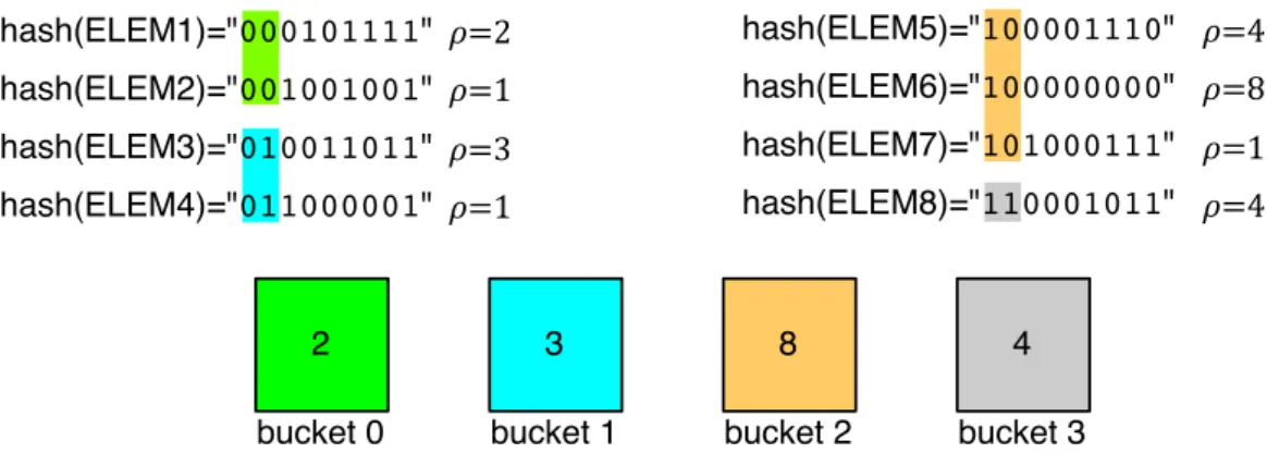
ρ(x) = 3 in 12.5% of the cases, . . . ). Figure 2.1 shows the behavior of these algorithms, but for ease of representation instead of small bit arrays it uses integers to represent the buckets.
Linear Counting Sketches
Linear Counting (LC) Sketches [53], on the other hand, use a single bit array/sketch
with size m. This sketch is initialized with 0s. When an item i is to be inserted, its
hash value hi, is used to calculate an index within the sketch (mod(hi, m)), which
2.2. ALGORITHMS AND DATA STRUCTURES 15
hash(ELEM5)="100001110"
hash(ELEM8)="110001011" hash(ELEM7)="101000111" hash(ELEM6)="100000000" Lets assume m = 4, therefore k = 2
2 3 8 4 hash(ELEM1)="000101111" hash(ELEM4)="011000001" hash(ELEM3)="010011011" hash(ELEM2)="001001001" 𝜌=2 𝜌=1 𝜌=3 𝜌=1 𝜌=4 𝜌=8 𝜌=1 𝜌=4
bucket 0 bucket 1 bucket 2 bucket 3
Figure 2.1: Insertion of elements in a (Hyper)LogLog Sketch
algorithm uses the fraction of empty sketch entries (Vn). In order to obtain this
value, it counts the number of empty sketch entries (the number of 0 entries in the sketch) and divides it by the total size of the sketch. The key concept behind LC Sketches is that for a uniformly distributed hash function, it is expected for the fraction of zero bits in the sketch to be inversely proportional to the number of distinct elements in the multiset. LC Sketches’ name comes from their linear space
complexity O(Nmax) (where Nmaxis the maximum number of different elements
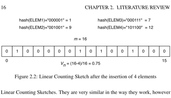
that the sketch can hold), i.e. their size grows linearly with the number of distinct elements that can be hold. Compared to (Hyper)LogLog Sketches, LC Sketches’ space complexity is a drawback, specially for multisets with large numbers of distinct elements. However, LC Sketches are easier to implement and also provide better estimates in multisets with a small number of distinct elements. Figure 2.2
shows a LC Sketch with size m= 16, after the insertion of 4 elements, Vn = 0.75.
Notice that “ELEM4” is inserted in index i = 12 because that is the remainder of
the integer division of 44 over 16.
Robust Network Aggregation Linear Counting Sketches and Robust In-Network Aggregation Dynamic Counting Sketches
Both Robust In-Network Aggregation Linear Counting Sketches (RIA-LC) [21, 20] and Robust In-Network Aggregation Dynamic Counting Sketches (RIA-DC) [20] are based on LC Sketches. RIA-LC sketches are a slightly improved version of
16 CHAPTER 2. LITERATURE REVIEW 1 0 0 0 0 0 1 0 1 0 0 1 0 0 0 0 hash(ELEM1)="000001" = 1 hash(ELEM2)="001001" = 9 hash(ELEM3)="000111" = 7 hash(ELEM4)="101100" = 12 0 15 m = 16 Vn = (16-4)/16 = 0.75
Figure 2.2: Linear Counting Sketch after the insertion of 4 elements
Linear Counting Sketches. They are very similar in the way they work, however RIA-LC Sketches are less prone to the overflow problem that occurs in LC Sketches when all the bits in the sketch are set to 1.
One of the major issues with all of the previous algorithms is the merge opera-tion. All of them allow the merging of several sketches of the same type to obtain an aggregate count of the number of distinct elements. However, all the sketches to
be merged must be similar (same size/accuracy). Furthermore, each of them has
to be big enough to hold the aggregate number of distinct elements. For instance, given two sketches with no overlap between their elements, with 200 and 10000 distinct elements, if we plan on computing their aggregate then each sketch must
be big enough to hold at least 10200 elements. RIA-DC sketches don’t suffer from
this issue. They have the ability to merge sketches of different sizes. However, this
ability comes with a price. RIA-DC Sketches assume that elements belonging to
different sketches do not overlap, meaning that if we merge two different RIA-DC
sketches with elements in common, those elements will be counted twice in the final aggregate.
2.2.2
Bloom Filters
Bloom Filters (BFs) were created in 1970 [9] by Burton Howard Bloom. They are
a simple and space efficient data structure for set representation where membership
queries are allowed. Bloom Filters allow false positives but do not allow false negatives, i.e, when querying a Bloom Filter about the existence of an element in a given set, if the answer is no, then the element is definitely not in the set, but if the
2.2. ALGORITHMS AND DATA STRUCTURES 17 answer is yes, the element might be in the set.
A Bloom Filter for representing a set of n items S = {x1, x2, x3, ..., xn} is
tra-ditionally implemented using an array of M bits, all initially set to 0. Then, k
independent hash functions are used {h1, h2, ..., hk}, each one mapping the element
of the set into a random number uniformly distributed over the range {1, ..., M}. For
each element x of the set (x ∈ S ) the bits of the positions hi(x) are all set to 1 for
1 ≤ i ≤ k. A location can be set to 1 multiple times. Due to the independence of the hash functions, nothing prevents collisions in the outputs. In extreme cases it
is possible to have h1(x)= h2(x)= ... = hk(x). To prevent this, we use the variant
of Bloom Filters presented in [10] which partitions the M bits among the k hash
functions, creating k slices of m= M/k bits. This ensures that each item added to
the filter is always described by k bits. Given a Bloom Filter BFS, checking if an
element z ∈ BFS, consists in verifying whether all hi(z) are set to 1. If they aren’t,
then z is definitely not present on the filter. Otherwise, if all the bits are set to 1,
then it is assumed that z belongs to BFS although that assumption might be wrong.
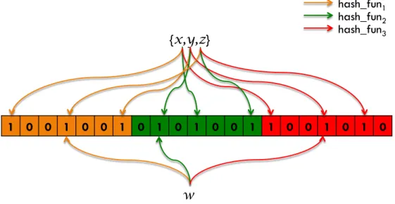
This false positive probability exists because the tested indices might have been set by the insertion of other elements. Figure 2.3 illustrates such an example.
Bloom Filters
12
1 0 0 1 0 0 1 0 1 0 1 0 0 1 1 0 0 1 0 1 0
{x,y,z}
Checking if w belongs to the set
w
hash_fun2
hash_fun3
hash_fun1
Figure 2.3: Bloom Filter with k = 3, M = 21 and m = 7, containing elements
{x, y, z}. Querying for the presence of element w yields a false positive.
18 CHAPTER 2. LITERATURE REVIEW is the ratio between the number of set bits in the slice and the slice size m. The fill ratio p can be obtained through equation (2.2).
P= (1 − p)k (2.1)
p= 1 − 1 − 1
m !n
(2.2) Furthermore, given a maximum false positive probability P, and the number
nof distinct elements to store, equations (2.3) and (2.4) can be used to estimate
the optimal number of bits required by a Bloom Filter to store those n elements,
M = m ∗ k. k= log2 1 P ! (2.3) m= n ∗ |lnP| k ∗(ln2)2 (2.4)
Counting Bloom Filters
Counting Bloom Filters (CBFs) were presented in [19] although they were only given this name later in [43]. They were introduced in order to allow the deletion of elements from the Bloom Filters. Suppose that we have a set that changes over time, where elements are inserted and deleted. The insertion of elements can be easily done using a normal Bloom Filter, hash the element k times and set the bits to 1. Unfortunately the delete operation cannot be accomplished simply by reversing the process. The resulting positions from the hash functions cannot be set to 0, because each position may be hashed by some other element from the set.
In a Counting Bloom Filter, each position is a small counter rather than a single bit. When an item is inserted the corresponding counters are incremented, and when the item is deleted the same counters are decremented. We just have to
2.2. ALGORITHMS AND DATA STRUCTURES 19 Scalable Bloom Filters
As we have seen, Bloom Filters provide space-efficient storage of sets at the cost
of a probability of false positives on membership queries. A conservative approach is usually chosen when filters are created because in case the number of elements stored surpasses the original number that the filter was supposed to hold, the false positive probability starts to increase rapidly. That conservative approach usually leads to filters orders of magnitude larger than needed and consequently to wasted space. To tackle this issue, Almeida et al. [2] introduced the concept of Scalable Bloom Filters (SBF), a variant of Bloom Filters that can adapt dynamically to the number of elements stored while respecting a maximum false positive probability, which is chosen in the beginning. SBF are a mechanism that adapts to growth of sets using a series of classic Bloom Filters of increasing sizes and tighter false positive probabilities. When the filters get full, a new one with
size = previous size ∗ growth rate and tighter false positive probability is made.
To check for the presence of an element, one has to query all filters.
2.2.3
Vector Clocks
Broadly speaking, a distributed system consists in a set of processes connected through a network. Each of these processes’ internal state can only change through the occurrence of events. There are 3 kinds of events: message sending, message reception and state transition events deriving from the normal execution of the process. In a distributed system, processes can only communicate using message passing as there is no shared memory. In this context and considering the ordering of events in an asynchronous model (since no assumptions should be made about timing), several strategies to cope with this asynchronicity were devised. One of the most prominent is vector clocks.
In order to better understand how Vector Clocks work, we must first comprehend the concept of causality. Causality is a relation through which we can connect two
events, a first event (known as the cause) and a second one (the effect).
In the context of Distributed Systems, causality is expressed using the
happens-beforerelation [38] denoted by the → symbol. For instance, given 2 events, x → y,
20 CHAPTER 2. LITERATURE REVIEW The happens-before relation has the following properties over any given event: • ∀a, b, c if a → b and b → c, then a → c (transitivity);
• ∀a, a 9 a(irreflexivity)
• ∀a, b if a → b then b 9 a (antisymmetry)
Therefore, it is a strict partial order over sets of events.
Vector Clocks were introduced by Colin Fidge [33] and Friedemann Mattern [41] in 1988 and are a practical implementation of the happens-before concept. In
this algorithm, each process Pi has a vector of integer values VCi[1..n] where n is
the number of processes, maintained by the following set of rules: 1. In the beginning, all the positions from the vector are set to 0
2. Each time the state of a process Pi changes (send, receive or internal event),
it must increment the value VCi[i], i.e, (VCi[i]= VCi[i]+ 1).
3. Each time a process Pisends a message, its vector VCishould be enclosed
in that message.
4. When a process Pi receives a message m, it must update its vector using the
formula: ∀x : VCi[x]= max(VCi[x], m.VC[x]), where m.VC symbolizes the
vector clock attached to m.
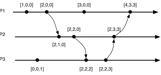
Figure 2.4 shows a concrete example of the above rules in a distributed system with 3 processes.
Vector Clocks are able to accurately represent the causality relation and the partial order it defines. Given any two distinct events x and y:
∀(x, y) : (x → y) ⇐⇒ (VCx < VCy)
Where VCx < VCy stands for:
(∀k : VCx[k] ≤ VCy[k] ∧ (∃k : VCx[k] < VCy[k]))
An important property of this mechanism is the result by Charron-Bost [11] proving that Vector Clocks are the most concise characterization of causality among process events.
2.2. ALGORITHMS AND DATA STRUCTURES 21 P1 P2 P3 [2,2,0] [2,2,3] [0,0,1] [2,2,2] [2,1,0] [2,3,3] [1,0,0] [2,0,0] [3,0,0] [4,3,3]
3
Collaborative Gate Counting
In this chapter, we tackle one of the most common forms of urban sensing: counting unique visitors across multiple gate counters to measure the number of people across the urban setting.
3.1
Motivation and System Model
Bluetooth scanners register the Bluetooth addresses, 48-bit MAC, of the devices that have been sighted. The Bluetooth device address is a 48-bit MAC format address that uniquely identifies each Bluetooth device. Some devices are able to switch between multiple Bluetooth addresses, but for most cases this will be a reliable and permanent unique identifier for sighted devices and by extension to the respective owners. A single scan of nearby devices is not in itself much of a problem. However, a systematic registration of Bluetooth sightings, especially when done at multiple locations, has the potential to become a large scale tracking system given the personal nature of most Bluetooth devices. Relatively simple processes can be put in place to detect the presence, movements and patterns of individuals. Concerning anonymity, the absence of a public record mapping Bluetooth addresses to specific individuals is nothing but a fragile barrier. To track
a specific individual, it would suffice to intersect the Bluetooth addresses from
some of the places she has visited. Eventually, all that would have been left is a 23
24 CHAPTER 3. COLLABORATIVE GATE COUNTING single Bluetooth address which could then be used to easily track that person from that moment on. To prevent cases like this, a privacy preserving approach should avoid permanent storage and dissemination of Bluetooth addresses or of any other information that could uniquely identify an individual.
Our Gate Counting scenario assumes the existence of a large set of hetero-geneous and autonomous Bluetooth nodes. We use the terms node and scanner interchangeably throughout this document. Conceptually, a gate is a virtual line across a street, and gate counting is the process of counting the number of people crossing that line. Each Bluetooth node is modeled as a gate counter that counts the number of unique Bluetooth addresses observed during a certain period.
A Bluetooth-based gate counter does not really count all the people passing-by, but only those who are carrying discoverable Bluetooth devices. Still, this is enough to make a reasonable correlation, using baseline data to estimate the
overall traffic. A gate counter should recognize subsequent sightings of the same
entity. In a gate counting scenario, repeated sightings of the same device can be very common because of persistent devices. Instead of scanning through a line, Bluetooth discovery is actually performed in an area and thus any device in that area, possibly in nearby buildings, would be repeatedly discovered. Furthermore, results from empirical studies with known static and transient devices suggest that a transient device typically appears for up to 90 seconds while it crosses a gate [46]. A proper gate counting process needs to account for these facts and filter both the persistent and repeated transient devices. A good way to do this is to count the number of unique devices.
A gate counter should also be able to answer questions like “how many different
people were seen in a given gate in the last 24 hours?” or “what was the number of visitors of an amusement park during visitors peak hours?”. To comply with this requirement, gate counters should be able to distinguish its readings over time.
The main challenge, however, is how to enable collaborative counting between multiple independent gate counters, while providing appropriate privacy guarantees as well as low communication costs. To be able to count unique entities, we need to
identify multiple counts of the same entity at different nodes, to make sure that the
same device sighted at two different gates will be counted only once. Imagine, for
3.2. CRITERIA 25 to count the number of visitors to the festival. The simple sum of individual gate counts would clearly overestimate the number of people since many of them would be spotted at multiple gates. Thus, we need some technique that works across multiple gate counters and is able to provide an aggregate count of the unique devices that have been spotted in the entire set of gate counters. Comparing the
plain addresses observed at different gates would immediately solve this problem,
but as we have seen, it is not suitable for privacy preservation.
3.1.1
Objectives
In this chapter, we explore the use of stochastic summarizing techniques as a privacy preserving approach to enable Bluetooth-based gate counting of unique entities across multiple nodes. The objective is to assess the extent to which these techniques are able to address the specific requirements of this distributed gate counting model, and inform the design of large scale Bluetooth sensing systems.
Having identified the sensing requirements for this scenario we have established a number of key criteria for assessing the various alternatives. Using those criteria, we have conducted an experimental study in which we compared how multiple types of stochastic summarizing techniques would behave across multiple variants of our gate counting scenario. The results provide a strong foundation for the development of these large scale Bluetooth sensing infrastructures, identifying
major trade-offs and the implications of key factors such as cardinality and support
for merge operations.
3.2
Criteria
This section tests some of the techniques mentioned in Section 2.2, namely LogLog Sketches [17], HyperLogLog Sketches [57], LC Sketches [53], RIA-LC Sketches, [21, 20], RIA-DC Sketches [20], Bloom Filters [9] and Scalable Bloom Filters [2]. These techniques where picked because they provide an interesting solution to the gate counting problem. Probabilistic counters are flexible enough for estimating the overall number of unique sightings with some controllable accuracy, without ever keeping the plain Bluetooth addresses.
26 CHAPTER 3. COLLABORATIVE GATE COUNTING The requirements identified in section 3.1 boil down to three important criteria: accuracy, size and aggregation. These criteria were used in the evaluation the proposed techniques.
Accuracy
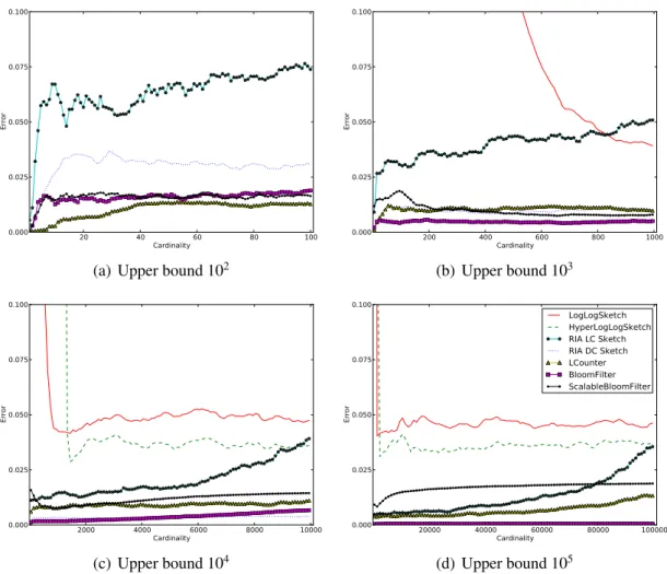
With this criterion we want to evaluate the accuracy of the techniques, their ability to count multiple sightings of the same device only once, and the quality of their estimators. To do so, we stipulated the maximum standard error for each technique. In this case after setting it to 5%, we measured for all techniques the relative error (root mean square error) for a range of cardinalities, whose average of 100 runs is shown in Fig 3.3.
Size
The size of the techniques is an important factor. The less space the technique requires, the lower will be both the costs of communication between BT scanners and their memory requirements.
Regarding this criterion, we have 2 fundamentally different types of techniques:
dynamic techniques which consist of Scalable Bloom Filters and static techniques comprising the rest. Static size techniques are techniques whose size is set at the time of creation and cannot be changed afterwards. This means that we must know the maximum number of unique devices to count before hand, or at least, we must be able to assume an upper bound for that number. Dynamic techniques on the other hand don’t have this drawback because they can adjust to withstand arbitrarily large cardinalities. In practical terms this means that for static size techniques, once we create an instance with a certain capacity it is not possible to change that capacity afterwards, while for dynamic techniques there is no such constraint.
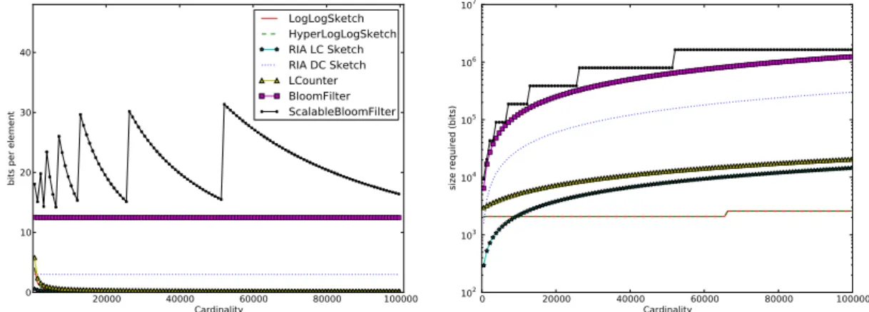
To further help us in our analysis, we can look at Figure 3.4. Figure 3.4(a) depicts the number of bits per unique element that each technique requires along a range of cardinalities. Figure 3.4(b) shows the total size spent by each technique to store a given number of distinct elements.
3.2. CRITERIA 27 Aggregation
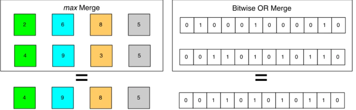
The ability to merge counts is crucial for scenarios with multiple gates. It is a key ingredient for obtaining the aggregate number of individuals in a set of gates. The merge operation (Figure 3.1) consists in either a bitwise OR operation (Bloom Filters, Linear Counting, RIA-DC and RIA-LC sketches) or in a max operation (HyperLogLog and LogLog sketches) of structures that make each gate’s counter. In order to merge several gate counters, there are 2 conditions that must be met: all counters must be instances of the same technique and every instance must have the same parameters and capacity (equally sized bit arrays). Meeting these conditions ensures that the same unique device will mark the same positions in the several gate counters it crosses. Therefore after merging the counters, it is possible to obtain the aggregate number of unique elements without counting the same device repeatedly (Figure 3.2). 2 6 8 5 4 9 3 5 4 9 8 5 max Merge
=
(a) max Merge- used by LogLog and Hyper-LogLog Sketches 1 0 0 0 1 0 0 0 0 1 0 0 0 1 1 0 1 0 1 0 1 1 0 0 Bitwise OR Merge
=
0 1 1 0 1 0 1 0 1 1 0 0(b) Bitwise OR Merge - used by Bloom Filters, RIA-LC, RIA-DC and LC Sketches
Figure 3.1: Different Merge Approaches
With the exception of Scalable Bloom Filters and RIA-DC sketches, all the techniques presented here have the ability to merge, and therefore will not count the same device more than once in aggregate counts. Scalable Bloom Filters lack the ability to merge because their size varies dynamically with the number of unique elements, therefore we cannot guarantee that the same unique device will set the
same positions for different filters. RIA-DC sketches might not provide accurate
aggregate results since the estimator considers there is no overlap of elements
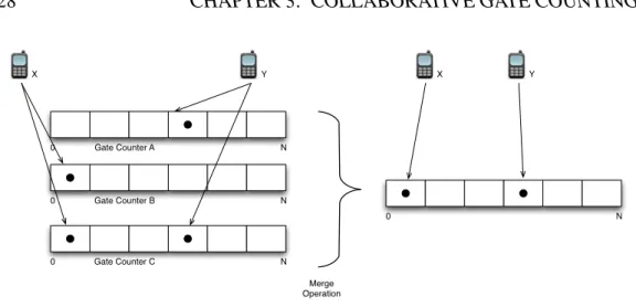
28 CHAPTER 3. COLLABORATIVE GATE COUNTING N 0 N 0 N 0 Gate Counter A Gate Counter B Gate Counter C N 0 Merge Operation X Y X Y
Figure 3.2: Gate Counter Aggregation - repeated devices appear only once
Aggregation is also important as a mean for answering time related questions
like “how many different people were seen in a given gate in the last 24 hours?” or
“what was the number of visitors of an amusement park during visitors peak hours?”.
To answer these types of questions, it must be possible to distinguish/segment
counter readings over time. This can by accomplished by sensor nodes periodically making a copy of their counters followed by a reset. Those copies will keep the information about the unique devices sighted during a certain time period. For example, considering that the rate at which counters are saved and reset is 1 hour, the former question could be answered by merging the 24 last saved counters. To answer the latter, we would need to merge the copies made during peak hours at the various nodes in the park.
To save some space, we can use different time granularities. For instance, we
can merge all unique counters saved during a day and obtain the aggregate count for the day, merge the counters from the last 7 days and get the aggregate count for the week, and so forth. We just need to keep in mind that because of the merge restrictions, the size of the counter that stores the unique number of devices sighted during an hour has to big enough to fit the number or unique devices seen during the entire week.
As we can see, both time segmentation and aggregate counting are in fact variations of the same problem, which can only be solved with techniques that support merging.
3.3. EVALUATION 29 20 40 60 80 100 Cardinality 0.000 0.025 0.050 0.075 0.100 Error
(a) Upper bound 102
200 400 600 800 1000 Cardinality 0.000 0.025 0.050 0.075 0.100 Error (b) Upper bound 103 2000 4000 6000 8000 10000 Cardinality 0.000 0.025 0.050 0.075 0.100 Error (c) Upper bound 104 20000 40000 60000 80000 100000 Cardinality 0.000 0.025 0.050 0.075 0.100 Error LogLogSketch HyperLogLogSketch RIA LC Sketch RIA DC Sketch LCounter BloomFilter ScalableBloomFilter (d) Upper bound 105
Figure 3.3: Relative error of the several techniques using various upper bounds. Average of 100 runs.
3.3
Evaluation
Using the results from our benchmark1 shown in figures 3.3 and 3.4 and having
explained the different criteria we can now analyze each one of the techniques.
Standard and Scalable Bloom Filters
Both techniques provide a good accuracy for all the cardinalities tested, never surpassing the stipulated relative error. Figure 3.3 confirms both these facts.
How-1Our Benchmark was built in Python, including the implementation of the several algorithms,
30 CHAPTER 3. COLLABORATIVE GATE COUNTING 20000 40000 60000 80000 100000 Cardinality 0 10 20 30 40
bits per element
LogLogSketch HyperLogLogSketch RIA LC Sketch RIA DC Sketch LCounter BloomFilter ScalableBloomFilter
(a) Number of bits per element used by each tech-nique at different cardinalities
0 20000 40000 60000 80000 100000 Cardinality 102 103 104 105 106 107
size required (bits)
(b) Size of the several techniques for different cardi-nalities
Figure 3.4: Size benchmarks
ever, looking at Figure 3.4 we can confirm that in regard to space, they are the most expensive techniques of all. This extra cost in terms of space stems from their query membership ability. Figure 3.4 also highlights the incremental nature of Scalable Bloom Filters. Each time the filter gets full, a new Bloom Filter is created, increasing the size of the technique. This explains the seemingly strange behavior of the technique. Both these techniques are also the most computationally expensive of all in terms of insertion complexity.
LogLog and HyperLogLog Sketches
As depicted by Figures 3.3(a) and 3.3(b), these techniques have very low accuracy
for small cardinalities (. 1800). Apart from this issue, they are the best suited
techniques for large cardinalities due to their logarithmic growth in size. As shown in Figure 3.4(b), for numbers of distinct elements above 10000, these are the most
efficient techniques in terms of space. Between the two, HyperLogLog sketches
have the advantage of being more accurate and of having a smaller variance. Regarding insertion complexity, these techniques are less expensive than Bloom Filters, but more expensive than the LC Sketches based ones.
3.4. SUMMARY 31 LC Sketches, RIA-LC Sketches and RIA-DC Sketches
Spending only a little more memory than LogLog Sketches, LC Sketches do not
suffer from poor accuracy in smaller cardinalities, they have an all around good
accuracy just like Bloom Filters. LC Sketches are a good all around technique. Be-ing based on Linear CountBe-ing Sketches, it is no surprise that RIA-DC and RIA-LC Sketches also have good accuracy results. Furthermore and like their ancestor, they also achieve good results in the bits per element ratio. These techniques are also the ones with the smallest complexity in terms of element insertion.
Taking into account all that has been said, there are a few conclusions to be drawn. For scenarios where we cannot make assumptions on the maximum number of elements to count, we have to use Scalable Bloom Filters. For scenarios where
there is a big discrepancy between the cardinalities of different counters and where
the existence of repeated elements outside each counter can be neglected, RIA-DC Sketches are probably the best choice. For scenarios with very large cardinalities HyperLogLog Sketches are probably the correct choice since they are the most
space efficient technique. Considering the expected most common scenarios, where
we need accurate aggregate counts and where there is the possibility of counters with low cardinalities, the choice falls either within Linear Counting Sketches or RIA-LC Sketches. We prefer the latter since it is a slightly simplified version of the former.
As a final remark, we should emphasize the fact that all the techniques discussed
in this chapter are more efficient in terms of space than storing each unique device’s
48 bit MAC address (check Fig.3.4(a)).
3.4
Summary
Bluetooth devices are pervasive in most societies and the number of unique Blue-tooth sightings is an adequate proxy for the number of actual individuals present. The trivial approach of collecting and counting the set of detected Bluetooth MAC addresses is not adequate, in most settings, both in terms of privacy concerns,
32 CHAPTER 3. COLLABORATIVE GATE COUNTING system scalability and adequacy to devices with limited memory.
In this chapter we described and benchmarked a set of stochastic summarizing techniques that can be applied to the gate counting problem. By using these techniques our approach ensures the privacy of the users since Gate Counters don’t store any extra raw information, i.e., the raw information that they keep at any given moment is also present in the Bluetooth network.
Furthermore, the analysis of these techniques and their trade-offs should help
4
Causality Tracking
This chapter, addresses the use of Bluetooth sightings as a way to acquire knowl-edge about the movement patterns of people. To do so, we propose a new technique with adjustable accuracy capable of representing the causality relation between visited places.
4.1
Motivation and System Model
The use of hash functions is often suggested as a data sanitation technique in which a Bluetooth address is replaced by a digest from which it is not be possible to recreate the original address. However, this is also not suitable for large scale BT sensing. It would be possible, even with minimal information about someone, to identify the respective digest, and from that point onward, the digest would again function as a unique identifier (pseudonym).
There are examples, such as the Netflix case [45], that show how surprisingly easy it can be to personalize information that was being proposed as anonymous (quasi-identifier [8]) simply by adding some basic additional knowledge to the system. This is also visible in other domains [47]. Therefore, the systematic registration of Bluetooth sightings done at multiple locations constitutes a privacy threat in that it allows the creation of a surveillance system for people.
The use of Bluetooth as an enabling technology to establish the flows of people 33
34 CHAPTER 4. CAUSALITY TRACKING is not a new concept. There are several examples, be it within a city [46], outdoor festival [51] or shopping mall [42].
The model in which we base our work assumes the existence of a network of heterogeneous and autonomous nodes that collaborate in the tracking process of Bluetooth devices. These nodes may have access to various types of information about the devices: their MAC address, the timestamp of the sighting, the type of Bluetooth protocols supported by the devices, among others.
Similarly to the Gate Counting scenario in Chapter 3, there is the possibility of using preexisting resources (nodes). As a consequence, our model does not impose restrictions on the type of information registered by the scanners. The nodes will continue to perform the same functions they did before. Our concern is to the information that might be exchanged by the nodes in the context of collective tracking, and to the privacy risks that might ensue such as the ability to accurately follow the movement of a device and therefore of its respective owner.
In their everyday life and depending on their specific needs, people visit several
different places. For instance, a person P1 wants to buy a new laptop. To do so,
she visits store S1which does not have the model she wants. She then visits store
S2 which is out of stock and afterwards store S3 where the price is a little steep.
She ends up buying the laptop in store S4. To represent this behavior we introduce
the concept of mobility traces. A mobility trace is simply the representation of the places visited in the order by which they were visited. In this specific case,
the mobility trace of P1is MTP1 = {S1, S2, S3, S4}. Our mechanism, Precedence
Filters, allows the recording of information relative to the individual traces of people, in a manner compatible with plausible deniability. That information can
later be processed/mined to obtain more accurate data about the habits of the
aggregate of all individuals. For instance, in this example, the order in which the
stores were visited might be an indicator of their reputation/popularity.
A common strategy that seeks to strengthen privacy is the restriction of captured data to just the essential. In our specific case, the goal is the detection of movement
patterns between nodes. As such, the ability to detect the same device on different
nodes is fundamental. To minimize the amount of information collected, we can ignore information such as the duration of the sightings, the timestamp in which they occurred, the device name, supported Bluetooth protocols, among others. We
4.1. MOTIVATION AND SYSTEM MODEL 35 just need the device’s MAC address.
Whenever a device is sensed, the sighting node records that event locally. This information is then used in the computation of device transitions between the system’s multiple nodes. The place where that computation occurs depends on the system’s architecture. Our mechanism can be deployed in either centralized or decentralized architectures. In a centralized system configuration, the computation has to be done in the server since only it has enough information to do so. Each node only shares its local information with the server. On the other hand, with a decentralized architecture, nodes can do the processing locally. The local infor-mation each node possesses is shared with the other nodes, thus allowing all the nodes to have access to the data. Both models have advantages and disadvantages. For instance, the centralized approach is not fault tolerant, if the server crashes the tracking system stops working. This does not happen in the decentralized approach given that the same information is stored in multiple nodes (redundancy). The system can keep on working even if some of the nodes fail. Compared to the centralized version, the decentralized model also has greater availability as a result of the information redundancy. However, as a consequence of the exchange of information between all the nodes, the decentralized scenario has a bigger burden on the network when compared to the centralized one.
In order to achieve the goal we set ourselves, and taking into account the constrains presented by our model, our solution is based upon the following set of assumptions:
• Even though we cannot make assumptions about how each individual node will handle the observed Bluetooth addresses, our solution should never require the Bluetooth address or any other information that could uniquely identify individuals to ever leave the sensing node.
• No system element should, at any given time, have all the information necessary to accurately determine the path of a single individual.
• The aggregate result that a node can create about the set of all visiting devices should be accurate enough to be useful in human mobility observation scenarios, e.g. most common paths, similarity level between places.