A Work Project presented as part of the requirements for the Award of a Masters Degree in Economics from the NOVA – School of Business and Economics
CAN NATURAL DISASTERS IMPACT CHILDREN GROWTH PATHS? EVIDENCE FROM MOZAMBIQUE 2000 FLOODS
HELENA ISABEL ABREU VIEIRA RODRIGUES 826
A project carried out on the Development Economics course, under the supervision of: Professor Pedro Vicente
Abstract
Can natural disasters impact children growth paths? This research follows the current interest on the effects of large-scale natural disasters on human capital outcomes. We combine DHS Survey Data with GPS Data to study the impact of Mozambican major floods on children’s health outcomes. This particular flooding episode was caused by a combination of heavy tropical rainfalls and cyclone Eline taking place in early 2000. OLS and Propensity Score Matching are used to examine the causal relationship between household’s distance from flooded area and anthropometric outcomes of children. We conclude that for children born between 2000 and 2003, a kilometre increase in household’s distance leads to a 0.012 and 0.024 increase in the weight-for-age and weight-for-height z-scores, respectively.
Keywords: natural disasters, Mozambique, children’s weight and height 1. Introduction
Several decades past the first scientific consensus regarding climate change, economists still struggle with identifying the causal influence of environmental conditions on global patterns of economic development. And though studies show that natural disasters are in fact threatening to toll back years of sustained growth in several developing nations worldwide, much of the economic literature on growth and sustainable development has somehow maintained the reasoning that dollar for dollar is better to invest in growth than climate resilience strategies because growth is the best solution for natural disasters.
According to UNISDR, water-related disasters are becoming increasingly frequent. Flooding alone accounted for 47% of all water related disasters between 1995 and 2015, affecting 2.3 billions of people worldwide. About 95% of flood disasters occur in Asia. Thus, the majority of literature available also focus on Asian countries such as India and Bangladesh. This research contributes to the literature on water-related natural disasters in Sub-Saharan Africa, a region of the world highly susceptible to droughts, floods and cyclones.
Households living closer to flood-prone rivers are subject to higher variability in health outcomes. Furthermore, environmental changes affecting child’s immunization, nutritional intake and overall security, can have long-term effects and be transmitted to future generations through maternal health. Thus, it is important to quantify and understand the impacts of natural disasters on human capital in order to define strategies to cope with the increasing climate insecurity.
Mozambique’s geography includes ten main river systems and an extensive coastline. The country is susceptible to tropical cyclones, particularly in the period between January and March. Despite the high propensity for water-related disasters, in 1999, Mozambique’s response capacities were scaled down and information about flood management was lacking. In early 2000 the country witnessed the worst natural disaster in the last decades. It resulted from a combination of torrential rains beginning in late January and Cyclone Eline. Five international rivers were flooded (Buzi, Incomati, Limpopo, Pungue and Save rivers), at least 700 people died, 650,000 were displaced and 4.5 million were affected, totalling about a quarter of Mozambique’s population.
Our research takes advantage of the accepted exogeneity of major floods to study the impact of natural disasters on infants’ health outcomes. This approach is in accordance with current literature on natural disasters, which focus on large-scale events prone to foreign aid. The absence of pre-flood national disaster management strategies also helps ensure our results convey the real effects of the catastrophe. Following the disaster, public health measures helped avoid epidemic outbursts. Also, as expected, international emergency assistance was conceived to the Mozambican Government in a total of 160 million US dollars. This was essential to mitigate the long-term impacts of the floods.
We use households’ geo spatial location (GPS), to understand how proximity to flooded areas affects children z-scores. The affected areas were identified using satellite images from NASA, known as Radarsat satellite images. These correspond to time specific flood analysis maps, containing arithmetic latitudes and longitudes (“screenshots” of the actual flood sites in the end of February, 2000). Afterwards, we used Google Earth Software to collect river coordinates within the areas previously established. For each river area, points were collected along the river course with a distance of 1 kilometre between them and centred according to natural river width at that specific location.
Exploiting data from three different Demographic and Health Surveys (1997, 2003 and 2011), we test the hypothesis that after major flooding occurs, children living further away from flooded rivers are healthier, have higher z-scores, than those living closer to affected areas. In order to do so, we calculated the smallest geodetic distance between the household’s geographical location, either at village level (2011) or district level (2003), and any of the flood points. We then reduced the sample to observations whose distance is inferior to 50 kilometres, which corresponds to approximately 45% of the initial sample. Two different identification strategies are used to test the stated hypothesis, OLS and Propensity Score Matching.
Our results show that, for both econometric models used, the previously stated hypothesis holds true only in 2003 for children born between 2000 and 2003. For these children, a positive statistically significant linear relationship exists between the variable of interest and the weight-for-age and weight-for-height z-scores – an extra kilometre increases the z-scores by 0.012 and 0.024, respectively. For the propensity score matching exercise, we defined treatment as a binary variable assuming 1 if household’s distance is superior to 10 kilometres and 0 otherwise. Again, for the mentioned cohort, the average treatment effect for the age and weight-for-height z-scores is 0.744 and 1.077, respectively. This research finds no statistically significant impact of distance in z-scores of children born between 2006 and 2011 and between 1998 and 2000.
The rest of the paper goes as follows: Section 2 includes a brief literature review on the topics covered in this research; Section 3 presents a background on Mozambique and the specifications of the disaster; Section 4 presents the data used; Section 5 presents the identification strategies; finally, Section 6 includes the econometric results for both models as well as robustness checks for propensity score matching. The paper ends with a brief discussion of important conclusions drawn from the work presented.
2. Literature Review
Natural disasters are a recurrent event in developing countries, and there is increasing concern that they may become more common due to climate change (Aaalst 2006). Although science points to an underlying relationship between the increase of natural disasters and climate change, it has been challenging to identify the causal influence of environmental conditions on global patterns of economic development (Hansiang, Jina 2015). Detecting the influence of long-term climate change in households’ health is difficult because of the large variability in health outcomes and climate variables. In fact, the past couple of decades witnessed many relevant changes, directly affecting health outcomes, such as vaccination, some of which may conceal the negative impacts of environmental variations (Campbell-Lendrum Et al. 2000; Menne Et al. 2000). Furthermore, natural disasters do not impart all households equally. Literature available shows that risk management and coping strategies, which depend on access to well-functioning markets, are context dependent and vary by wealth levels (Carter Et al. 2004).
Our research follows the trend on available literature regarding the effects of natural disasters on children’s health, which is mostly oriented for individual large scale events. Examples include studies showing that the 1994-1995 drought in Zimbabwe slowed the growth of children under the age of two (Hoddinott, Kinsey 2001); forest fires in Southeast Asia increased infant mortality (Sastry 2002; Jayachandran 2006); Hurricane Mitch in South America decreased child’s health and nutrient intake while also increasing their labour force participation (Baez, Santos 2007); and children born of women exposed in childhood to the Tanzanian flood in 1993 have lower height-for-age z-score (Caruso 2015). These large-scale events tend to attract foreign aid more easily (Stroember 2007), which has the potential to mitigate unfavourable effects.
Besides the immediate impacts of natural disasters on health and mortality, long-term indirect health effects may sustain through different mechanisms such as income shocks and restricted
permanently alter health paths, leading to lower formation of biological human capital in early childhood (Hoddinott, Kensey 2011; Del Ninno, Lundberg 2005). For example, disasters can delay or interrupt children immunization or may induce household to divert income from children’s nutrition intake. An extensive literature indicates that infants’ socioeconomic conditions and health exhibit long-term influences on individual’s health and mortality (Galobardes Et al. 2004; Victora Et al. 2008; Haas 2008). Also, shocks to children health may be transmitted to future generations through reproductive outcomes. Short women, for example, have a greater risk of obstetric complications due to smaller pelvic size (WHO 1995).
There is little doubt that malnourished children tend to have more severe diarrhoeal episodes and associated growth faltering (Tomkins, Watson 1989; Victora Et al. 1990; Briend, 1990). Also, there is a known association between increased mortality and increased severity of anthropometric deficits (Toole, Malkki 1992). Studies on child development show that poor growth is associated with compromised development (Pollitt Et al. 1993), school performance and intellectual accomplishment (McGuire, Austin 1987). A study on Guatemalan infants shows that childhood stunting leads to a significant reduction in adult size (Martorell Et al. 1992). Reduced work capacity and economic productivity are two main consequences of small adult size resulting from childhood stunting (Spurr Et al. 1977).
At every stage in life, health is strongly associated with different indicators for socioeconomic status (SES) such as income, educational accomplishment and occupational status (Currie 2009; Cutlet Et al. 2012; Smith 1999). The association between income, or wealth, and health outcomes manifests itself from early on. For example, children born from low-income households have lower birth weight, are more likely to be born prematurely and face greater risk for chronic health conditions throughout their lives (Brooks-Gunn and Duncan 1997; Currie 2009). Furthermore, it is widely recognized that childhood health is associated with
future wealth outcomes and that adult individuals with higher incomes enjoy better health outcomes too (Currie 2009; Smith 1999; Deaton 2002).
3. Background
In 2002 Mozambique was one of the poorest countries in the world, listed 170th out of 173 countries in the United Nations Human Development Index (UNDP 2002). Sixty-nine percent of the population lived bellow the established poverty line of 0,40 US dollars per day. The World Bank considers that natural disasters, along with the social and economic impacts of HIV/AIDS, constitute one of the main risks to the achievement of Mozambique’s poverty reduction strategy. In the period between 1965 and 1998 twelve major floods, nine major drought and four major cyclone disasters took place (Maule 1999).
Mozambique’s geography includes ten main river systems, that cross the country and drain into the Indian Ocean, and an extensive coastline. The catchment areas of these rivers drain water from vast areas of Southern Africa. Besides the increased flood risks caused by tropical rainfall in the river catchment areas and dams, the country is also susceptible to tropical cyclones, particularly in the period between January and March.
Although the country has a high propensity for natural disasters, in 1999 a surprisingly small amount of literature existed on the analysis of flood-prone areas, flood impacts and potential mitigation and preparedness measures. As an example, only 16 of Mozambique’s 500 hydro-meteorological monitoring systems were properly working in 1997 (Maule 1999). Until the beginning of the millennium, disaster management was mainly a reactive process due to the instability and insecurity caused by political events (Maule 1999). The desire to move away from the war-time relief mode, following a prolonged civil war taking place after Independence, excluded calamity prevention from the country’s development efforts. At the same time, both
governmental agencies and NGOs scaled down their disaster response capacities, emphasizing coordination rather than delivery.
The early 2000 floods that occurred in the southern part of Mozambique resulted from a combination of torrential rains beginning in late January and the Cyclone Eline. The first heavy rain episode, by the end of January, caused flooding of the Incomati River, swamping of the country’s capital and neighbouring cities. A second heavy rain episode, affecting north-eastern South Africa and central Botswana, together with Cyclone Eline left much of Mozambique’s southern Gaza and central Inhambane provinces accessible only be air due to floods in the Limpopo River, Buzi River, Save River and Pungué River. At least 700 people died, 650,000 were displaced and 4.5 million were affected, totalling about a quarter of Mozambique’s population. International relief operations avoided greater loss of life.
Following the disaster, public health measures avoided measles and cholera epidemics. Also, the government of Mozambique made three successive appeals for emergency assistance during February and March 2000, totalling 160 million US dollar, which had a response over 100 percent. Foreign aid was essential to mitigate the damages caused by the floods.
4. Data
4.1 Demographic and Health Data
Data was collected from the Standard Demographic and Health Surveys available through The Demographic and Health Surveys Program (DHS). The sample used contains one recode for every child under the age of five born from women of reproductive age (15-49 years). Each recode contains data on specific household and maternal characteristics as well as the anthropometric measurements. Given the time span of this analysis, three surveys were used: 1997, 2003 and 2011. Since no observation in the 1997 survey contains geo spatial location, we use this survey simply as the base year for descriptive statistics. For 2003, the question “district for health
facility” was used to obtain district level geospatial information for 1027 observations. The 2011 survey includes GPS data for each cluster in a total of 4618 observations. Cluster coordinates, for different groupings of households that participated in the survey, are collected in the field using GPS receivers during the survey sample listing process. These are accurate to less than 15 meters. In order to ensure that respondent confidentiality is maintained, the program randomly displaces the GPS latitude/longitude positions for all surveys, including those that do not have HIV testing. This is done so that: urban clusters contain a maximum of 2 kilometres and a minimum of 0 kilometres of error; rural clusters error varies between 0 kilometres and a maximum of 5 kilometres with a further 1% of the rural clusters displaced a between 0 and 10 kilometres.
4.2 WHO Child Growth Standards
Growth charts are a common measure to evaluate child growth trajectories and policies designed to improve child health. The World Health Organizations charts, released in April of 2006, are based on a prospective international sample of children chosen to represent optimal growth in supportive environments. The WHO database uses, as basis for comparison of anthropometric data across countries, the National Center for Health Statistics (NCHS) growth reference curves, formulated in the 1970s by combining growth data from two distinct data sets: the reference for ages 0-23 months is based on a group of children from the Ohio Fels Research Institute Longitudinal Study, which was conducted from 1929 to 1975; the reference from 2-18 years old is based on data from three cross-sectional USA representative surveys conducted from 1960 to 1975. All the reference samples consist of healthy, well-nourished American children.
This research uses z-scores to compare infants to the reference population. Z-score is widely recognized as the best system for analysis and presentation of child anthropometric data. It is also regarded as the most appropriate descriptor of malnutrition. The z-score system expresses anthropometric data as a number of standard deviations, referenced as z-scores, below or above
the reference median value. The formula for calculating the z-score is the following:
z-score = observed value – median value of the reference population standard deviation value of reference population
Z-scores have the same statistical relation to the distribution of the reference around the mean at all ages, resulting in comparable measures across age groups and different indicators. They are independent of age and sex, which allow us to compute means and standard deviations. Three different measures are used with z-scores: Weight for Age, Height for Age and Weight for Height. The WHO Global Database on Child Growth and Malnutrition uses a Z-score cut-off point of -2 standard deviations to classify low weight-for-age, low height-for-age and low weight-for-height. Low height-for-age is called “stunting” or “stunted growth” and low weight-for-height is called “wasting” or “thinness”.
4.3 Wealth Index Score
Social scientists have developed several approaches to assess the economic status of households, including consumption expenditures, income, assets and national gross domestic product (GDP) per capita. Wealth is a key indicator of well-being, health and social achievement. It is more permanent and easily measured than household consumption or income. Furthermore, measures of wealth are widely available in demographic and health surveys.
The current procedure for calculation of the DHS Wealth Index is described in detail in Rutstein (2008) but succinctly it involves first calculating a wealth index that uses items thought to be common and have common weightings in both rural and urban areas. Afterwards, area-specific wealth indexes are calculated for both areas. These area specific indexes include additional items above those included in the common wealth index, for example, the number of farm animals, agricultural land size and flush toilets or sewers. Then, for each area, predicted wealth scores are
calculated where the constant term of the regression adjusts the level of each area’s index relative to the common and the coefficient adjusts the dispersion in the distribution.
Each index has a mean value of zero and a standard deviation value of one. Specific scores cannot be directly compared across countries or over time. The DHS Program decided to include the DHS Wealth Index (Rutstein, Johnson 2004) as a standard recode variable in all DHS survey datasets from 2001 onwards. This justifies the absence of wealth index score for observations in the 1997 Standard DHS Survey used.
4.4 River Coordinates
Following the identification of each affected river, we used satellite images (Radarsat), provided by the NASA-supported Dartmouth Flood Observatory, to identify the arithmetic coordinates, latitudes and longitudes, within which floods occurred. These images have a spatial resolution of approximately 50 metres and correspond to flood analysis maps for the months of February and March of 2000, when the discussed floods took place. The satellite images work as screenshots of the affected areas for the specific moment in time and meteorological conditions described in Section 3.
Subsequently, we inputted these maps on Google Earth Software, establishing the limits for each flooded area. After each area was identified, coordinates were collected along the natural path of the river. Points were 1 kilometre spaced from each other and centred according to river width. 184 points were collected for the Save river; 83 points were collected for the Incomati river; 131 points were collected for the Limpopo river; 101 points were collected for the Buzi river; and, 154 points were collected for the Pungué river.
5. Empirical Strategy
This paper studies the relationship between household’s distance from flooded area and child z-scores. We test the hypothesis that after the flood takes place, children living further away from flooded areas are healthier, or have higher z-scores, than those living closer to river banks. Our variable of interest, household’s distance from flooded area, was defined as the smallest distance, measured in kilometres, between the household and one of the previously established river coordinates. Again, household location is measured at the district level in 2003 and village level in 2011. Also, distance corresponds to the geodetic distance (the length of the shortest curve between two coordinates along the surface of a mathematical model of the earth) calculated by means of the Vicentry (1975) equations on the WGS 1984 reference ellipsoid.
After distance was calculated, the sample was restricted to children living within 50 kilometres radius from any flood point. This reduces the final sample to 419 observations in 2003 and 1164 observations in 2011 – corresponding to approximately 45% of the original sample mentioned in Section 4. It allows us to diminish regional effects on child’s health outcomes.
Two different identification strategies were used to calculate the effects of the variable of interest on outcomes: OLS and Propensity Score Matching. The first model assumes a linear causal relationship between distance and the health outcomes of interest. Distance is a continuous variable and standard errors were clustered at village level for all regressions at the individual level. As an alternative to linear regression, a Propensity Score analysis (Rosenbaum, Rubin 1983, 1984; Rubin, 1997) was used to compare outcomes between treated and non-treated units. In this model, the distribution of observed covariates is independent of the binary treatment assignment (Rosenbaum, Rubin. 1983, 1984). Treatment is a binary variable assuming 1 if household’s distance is superior to 10 kilometres and 0 otherwise. We use a Logistic model to calculate the probability of treatment and Abadie-Imbens standard errors are reported. The Average Treatment Effects are calculated using a propensity score matching model with replacement.
This method is frequently used to deal with bias from standard regression in observational studies. We then have the following core specifications:
outcome' = α + β-T'+ β/X'+ ε' (1)
τ345 = α + β-T' + β/X' + ε' (2)
OLS results were calculated using specification (1). Specification (2) was used to calculate the Average Treatment Effect in Matching. The same set of controls was used for (1) and (2): urban residence dummy, household’s wealth score, mother’s education in years, mother’s weight and mother’s height. “urban residence” is a dummy for the de facto type of residence and assumes the value 1 or 0 if the household lives in an urban or rural residence, respectively. “wealth score” is the composite measure of household’s cumulative living standard described in Section 4. “mother’s education” is the mother’s education in years of schooling. “mother’s weight” is the mother’s weight measured in kilograms. “mother height” is the mother’s height measured in centimetres.
For 2003 two cohorts were established. Cohort 1 includes all infants born between 1998 and 2000. Cohort 2 includes all infants born between 2000 and 2003. This allows us to compare the health of children born before and after the event takes place.
6. Econometric Results
Table 1 and Table 2 contain the descriptive statistics, mean and standard deviation, for each variable of interest in each survey. Because of the lack of household’s wealth index data and geo-spatial identification, the 1997 DHS Survey is only used as a base for comparison.
From Table 1 we can see that mother’s education, weight and height increased throughout time. The impact of maternal education and anthropometrics on child’s health is better explained in the literature review. Household’s wealth score slightly decreased between 2003 and 2011.
Also, between 2003 and 2011 the percentage of people living in urban areas decreased by 18.2%.
Table 1: Descriptive Statistics
variables observations mean standard deviation
1997
Urban Residence, dummy 3 045 0.357 0.479
Mother's Education, years 3 040 2.384 2.822
Mother's Weight, kg 1 481 53.225 9.651
Mother's Height, cm 1 486 155.319 6.270
2003
Urban Residence, dummy 419 0.831 0.376
Household Wealth Score 419 1.011 1.144
Mother's Education, years 419 4.852 2.775
Mother's Weight, kg 405 58.787 10.754
Mother's Height, cm 404 158.179 5.813
2011
Urban Residence, dummy 1 164 0.649 0.478
Household Wealth Score 1 164 0.777 0.962
Mother's Education, years 1 164 5.552 3.589
Mother's Weight, kg 1 162 59.154 11.507
Mother's Height, cm 1 162 158.183 6.189
Table 2: Z-score Statistics
variables observations mean standard deviation
1997 Weight-for-Age z-score 3 045 -1.084 1.364 Height-for-Age z-score 3 045 -1.634 1.772 Weight-for-Height z-score 3 045 -0.207 1.450 2003 Weight-for-Age z-score 419 -0.484 1.017 Height-for-Age z-score 419 -1.332 1.125 Weight-for-Height z-score 419 0.344 1.117 2011 Weight-for-Age z-score 1 164 -0.395 1.117 Height-for-Age z-score 1 164 -1.154 1.476 Weight-for-Height z-score 1 164 0.371 1.204
Table 2 includes descriptive statistics for the different z-scores. Overall, there is a significant improvement in all z-scores between 1997 and 2011. Between 2003 and 2011, the averages of the weight-for-age and weight-for-height z-scores increased by 0.089 and 0.027, respectively. During the same period of time, the average of the height-for-age z-score decreased by 0.178, though it is still higher than in 1997.
For all tables from here onwards: columns (1) and (4) contain the estimates for the weight-for-age z-score; columns (2) and (5) contain the estimates for the height-for-weight-for-age z-score and columns (3) and (6) contain the estimates for the weight-for-height z-score.
In 2003, distance has a positive and significant impact in the age and weight-for-height z-scores - an extra kilometre distance from any flood point increases the z-scores by 0.013 and 0.021, respectively. In 2011, distance has a negative insignificant impact on children’s z-scores.
Mother’s weight, height and education are also very relevant in explaining child’s health outcomes. For example, an extra centimetre in mother’s height increases the height-for-age z-score by 0.054 in 2003 and an extra year in maternal education increases the same z-z-score, in 2011, by 0.033. Wealth also plays a significant role in explaining child’s z-scores, especially the height-for-age z-score in 2003 and the weight-for-age z-score in 2011. Finally, living in an urban residence seems to have a positive impact in 2003 and a negative impact in 2011, both are statistically insignificant nonetheless.
Table 4 includes the OLS estimates for both 2003 Cohorts. Cohort 1 is composed of children born between 1998 and 2000. Cohort 2 is composed of children born between 2000 and 2003. This exercise allows us to understand the differences in outcomes between children born before and after the event.
For the first Cohort, distance has a positive but insignificant impact in all children’s z-scores. Furthermore, living in an urban residence and mother’s weight have a very significant impact in the children’s weight-for-age and height-for-age z-scores. Specifically, an extra centimetre in mother’s height increases the z-score of children born between 1998 and 2000 by 0.104. For the second Cohort, a positive statistically significant causal relationship exists between the variable of interest and the weight-for-age and weight-for-height z-scores – an extra kilometre distance increases the z-scores by 0.012 and 0.024, respectively. Maternal anthropometrics and household wealth also have a positive and significant impact on these infants z-scores. For example, an extra kilogramme in mother’s weight increases the weight-for-age z-score by 0.021.
Table 3: OLS Estimates of the Effect of Distance From Flood on z-scores
2003 2011 (1) (2) (3) (4) (5) (6) Weight for Age z-score Height for Age z-score Weight for Height z-score Weight for Age z-score Height for Age z-score Weight for Height z-score
variables coef/se coef/se coef/se coef/se coef/se coef/se
Distance From Flood, km 0.013** -0.004 0.021*** -0.003 -0.004 -0.000 (0.006) (0.006) (0.007) (0.003) (0.005) (0.004) Urban Residence, dummy 0.167 0.192 0.084 -0.067 -0.112 -0.037
(0.144) (0.170) (0.189) (0.091) (0.162) (0.108) Household Wealth Score 0.073 0.149** -0.031 0.103* 0.107 0.063
(0.053) (0.059) (0.066) (0.057) (0.090) (0.061) Mother's Education, years 0.018 0.018 0.015 0.030*** 0.033** 0.017
(0.020) (0.025) (0.025) (0.011) (0.016) (0.012) Mother's Weight, kg 0.018*** 0.008 0.020*** 0.025*** 0.023*** 0.017*** (0.005) (0.006) (0.006) (0.004) (0.004) (0.004) Mother's Height, cm 0.023*** 0.054*** -0.009 0.006 0.031*** -0.014* (0.009) (0.009) (0.009) (0.006) (0.008) (0.007) No. Of Obs. 404 404 404 1162 1162 1162 r-squared adjusted 0.1436 0.1800 0.0732 0.1311 0.1082 0.0368 Note Table 3: All regressions are OLS. All dependent variables are z-scores. Standard errors are reported in parentheses; these are corrected by clustering at village level and geo referenced for 2011. For 2003, households are geo referenced at district level. * significant at 10%; ** significant at 5%; *** significant at 1%
Propensity Score Matching results are available in Table 5 and Table 6. The Average Treatment Effect (ATE) is the average causal effect of the dummy treatment variable on the outcome of interest. In this case, treatment is defined as the household’s distance being larger than 10 kilometres. These estimates add robustness to our previous findings.
The average treatment effect for 2003 is positive and statistically significant for the weight-for-age and weight-for-height z-scores. Treated children are on averweight-for-age better than untreated ones. The ATE for the weight-for-age and weight-for-height z-scores is 0.493 and 0.755, respectively. In 2011, the average treatment effects are negative and not statistically significant: -0,012 for weight-for-age z-score, -0,050 for the height-for-age z-score and -0,024 for the weight-for-height z-score.
Table 4: 2003 OLS Estimates of the Effect of Distance From Flood on Different Cohorts Cohort 1 Cohort 2 (1) (2) (3) (4) (5) (6) Weight for Age z-score Height for Age z-score Weight for Height z-score Weight for Age z-score Height for Age z-score Weight for Height z-score
variables coef/se coef/se coef/se coef/se coef/se coef/se
Distance From Flood, km 0.009 0.008 0.006 0.012* -0.008 0.024*** (0.010) (0.010) (0.010) (0.007) (0.007) (0.008) Urban Residence, dummy 0.814*** 1.145*** 0.143 0.018 -0.021 0.064
(0.298) (0.322) (0.251) (0.167) (0.209) (0.226) Household Wealth Score -0.079 0.067 -0.184 0.111* 0.175** 0.001
(0.113) (0.128) (0.113) (0.064) (0.070) (0.077) Mother's Education, years 0.010 -0.004 0.021 0.017 0.025 0.009
(0.050) (0.052) (0.045) (0.023) (0.029) (0.028) Mother's Weight, kg 0.010 0.003 0.014* 0.021*** 0.007 0.024*** (0.009) (0.011) (0.008) (0.007) (0.007) (0.007) Mother's Height, cm 0.057*** 0.104*** -0.011 0.017* 0.046*** -0.010 (0.016) (0.019) (0.016) (0.009) (0.010) (0.010) No. Of Obs. 78 78 78 326 326 326 r-squared adjusted 0.2931 0.4415 0.0651 0.1375 0.1542 0.0904 Note Table 4: All regressions are OLS. All dependent variables are z-scores. Standard errors are reported in parentheses; these are corrected by clustering at village level. Cohort 1 corresponds to children born between 1998 and 2000. Cohort 2 corresponds to children born between 2000 and 2003. * significant at 10%; ** significant at 5%; *** significant at 1%
Table 5: Estimates for PSM with replacement, Treatment distance superior to 10km 2003 2011 (1) (2) (3) (4) (5) (6) Weight for Age z-score Height for Age z-score Weight for Height z-score Weight for Age z-score Height for Age z-score Weight for Height z-score
variables coef/se coef/se coef/se coef/se coef/se coef/se
ATE 0.493*** -0.064 0.755*** -0.012 -0.050 0.024
(0.125) (0.162) (0.147) (0.078) (0.101) (0.091)
No. Of Obs. 404 404 404 1162 1162 1162
Note Table 5: Abadie-Imbens standard errors reported in parenthesis. Common support is established prior to each matching exercise by refining the sample after running logit regressions on restricted sub-samples. Controls are the same as in the OLS specifications. Standard errors reported in parentheses. * significant at 10%; ** significant at 5%; *** significant at 1%.
The average treatment effects for both cohorts in 2003 are presented in Table 6. For children born between 2000 and 2003 (Cohort 2), the ATE is positive and statistically significant for the for-age and for-height z-scores. Specifically, the average treatment effect for the weight-for-height z-score is 1.007. For the remaining children, born between 1998 and 2000, the average treatment effect is also positive but insignificant. This is in agreement with our previous OLS results.
Table 6: 2003 Cohorts - Estimates for PSM with replacement, Treatment distance superior to 10km Cohort 1 Cohort 2 (1) (2) (3) (4) (5) (6) Weight for Age z-score Height for Age z-score Weight for Height z-score Weight for Age z-score Height for Age z-score Weight for Height z-score
variables coef/se coef/se coef/se coef/se coef/se coef/se
ATE 0.320 0.189 0.324 0.744*** 0.002 1.077***
(0.225) (0.218) (0.202) (0.179) (0.160) (0.232)
No. Of Obs. 78 78 78 326 326 326
Note Table 6: Abadie-Imbens standard errors reported in parenthesis. Common support is established prior to each matching exercise by refining the sample after running logit regressions on restricted sub-samples. Controls are the same as in the OLS specifications. Standard errors reported in parentheses. * significant at 10%; ** significant at 5%; *** significant at 1%.
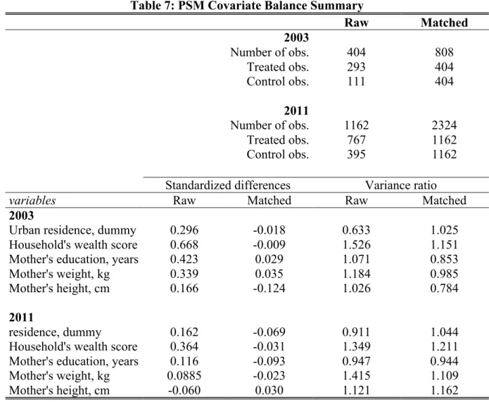
Possibly the most important step in using matching methods is to diagnose the quality of the resulting matched samples. So, we follow our analysis with an assessment of the covariate balance in the matched groups. Balance is defined as the similarity of the empirical distributions of the full set of covariates in the matched and treated groups.
One of the most common numerical balance diagnosis is the difference in means of each covariate, divided by the standard deviation in the full treated group. This measured is referred to as the “standardized bias” or “standardized difference in means” and is compared before and after matching (Rosenbaum, Rubin 1985).
Rubin (2001) presents three balance measures based on the theory in Rubin and Thomas (1997) that provides a comprehensive view of covariate balance. According to these measures, for a regression adjustment to be trustworthy, the absolute standardized difference of means should be less and 0.25 and the variance ratios should be between 0.5 and 2 (Rubin 2001). Ideally, a well-balanced covariate should have matched standardized difference of zero and a variance ratio of one. Though, there are no formal criteria generally agreed upon.
Table 7 contains the covariates balance summary for 2003 and 2011. For both years, residence and mother’s weight seem to be well balanced. Mother’s education seems to be better balanced in 2011 than in 2003. Household’s wealth score and mother’s height do raise same concerns regarding balance, though they still hold under the criteria defined by Rubin (2001). Problems with balance in 2003 may be related to the error associated with determining the GPS location at the district level and not at cluster level, like in 2011.
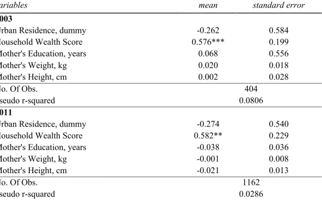
Table 8 includes the Logistic Estimation for the propensity of observations being assigned into the treatment group. In both years, individuals with a higher household wealth score are more likely to be living outside the 10 kilometres radius (be assigned to treatment).
Table 7: PSM Covariate Balance Summary Raw Matched 2003 Number of obs. 404 808 Treated obs. 293 404 Control obs. 111 404 2011 Number of obs. 1162 2324 Treated obs. 767 1162 Control obs. 395 1162
Standardized differences Variance ratio
variables Raw Matched Raw Matched
2003
Urban residence, dummy 0.296 -0.018 0.633 1.025
Household's wealth score 0.668 -0.009 1.526 1.151
Mother's education, years 0.423 0.029 1.071 0.853
Mother's weight, kg 0.339 0.035 1.184 0.985
Mother's height, cm 0.166 -0.124 1.026 0.784
2011
residence, dummy 0.162 -0.069 0.911 1.044
Household's wealth score 0.364 -0.031 1.349 1.211
Mother's education, years 0.116 -0.093 0.947 0.944
Mother's weight, kg 0.0885 -0.023 1.415 1.109
Mother's height, cm -0.060 0.030 1.121 1.162
Note Table 7: data included corresponds to posestimation diagnostic statistics. Treated observations include children whose household distance is superior to 10km. Control observations correspond to children whose household distance is inferior or equal to 10km.
Table 8: p-score for PSM
Logit Estimation for Treatment distance superior to 10km
variables mean standard error
2003
Urban Residence, dummy -0.262 0.584
Household Wealth Score 0.576*** 0.199
Mother's Education, years 0.068 0.556
Mother's Weight, kg 0.020 0.018
Mother's Height, cm 0.002 0.028
No. Of Obs. 404
pseudo r-squared 0.0806
2011
Urban Residence, dummy -0.274 0.540
Household Wealth Score 0.582** 0.229
Mother's Education, years -0.038 0.036
Mother's Weight, kg -0.001 0.008
Mother's Height, cm -0.021 0.013
No. Of Obs. 1162
pseudo r-squared 0.0286
Note Table 8: Treated observations include children whose household distance is superior to 10km. Control observations correspond to children whose household distance is inferior or equal to 10km. * significant at 10%; ** significant at 5%; *** significant at 1%.
7. Conclusion
The present work project was designed to contribute with empirical knowledge to economic literature about the causal influence of water-related natural disasters on human capital outcomes. We took advantage of the available data to prove that in the aftermath of a major flooding event, children living further away from flooded areas have higher z-scores.
Our results are very significant for children born in the three years following the event. This is because infants are much more vulnerable to changes that can compromise their nutritional intake, access to health and overall security. And although six years after the inundation takes place distance has no significant impact on child’s health outcomes, a long-term transmission mechanism of the effects of floods may take place through the form of maternal outcomes.
Overall, like in any empirical research, the absence of better geographical data prevented us from achieving more robust results in this work project. Although the DHS Program routinely collects geographic information in all surveyed countries, only recently researchers can link this data with routine health data, such as health facility locations, and environmental conditions. These data restrictions are particularly limiting when conducting a retrospective analysis. Regarding this specific work project, our main problem relies on the quality of the geo-spatial data in 2003. On one hand, we were forced to assume that all households living in the same district for health facility lived at the same distance from any flood point, which is a problematic simplification of our variable of interest. On the other hand, when conducting a research of this type in a sub-Saharan African country a researcher must be aware of the difficulties upfront. It is, in fact, difficult to encounter a better example to be examined – in terms of timespan since the event, the overall magnitude of damages and lack of initial coping strategies – despite the preliminary set of information available.
Obviously, even with today’s level of scientific knowledge, natural disasters are not completely predictable, which means randomization is not necessarily a feasible approach to calculating its impacts on households. In this particular case, in order to apply the propensity score matching method, we were forced to simplify our continuous variable of interest, which is a necessary but maybe an undesired simplification of our work.
Finally, this research allows us to make a solid argument in favour of both top-down and bottom-up approaches to natural disasters and climate change. On one side it is important for governments and international aid agencies to develop emergency relief operations that directly tackle children’s health and households’ wealth constraints in the aftermath of full-scale events such as the one studied. On the other side, equipping individuals with risk management strategies as well as access to financial instruments is essential to help populations in low-income countries deal with the long-term impacts of increased climate variability.
References
Alderman, H.; Hoddinott J.; Kinsey, B. 2006. “Long term consequences of childhood malnutrition.” Oxford Economic Papers 58(3): 450-474.
Briend, A. 1990. “Is diarrhoea a major cause of malnutrition among under-fives in developing countries? A review of available evidence”. European Journal of Clinical Nutrition. 44: 611-628. Brooks-Gunn, J.; Duncan, G. 1997. “The effects of Poverty on Children”. The Future of Children, 7: 55-71.
Campbell-Lendrum D.; Menne B., Wilkinson P.; Kuhn K.; Haines A.; Kovats S.; Bertollini R. 2000. “Monitoring the health impacts of climate change. Copenhagen”, WHO Regional Publications, European Series.
Caruso, G. 2015. “Intergenerational Transmission of Shocks in Early Life: Evidence from the Tanzanian Great Flood of 1993”. Working Paper.
Currie, J. 2009. “Healthy, Wealthy, and Wise: Socioeconomic Status, Poor Health in Childhood, and Human Capital Development”, Journal of Economic Literature, 47:87-122.
Cutler, D.; Lleras-Muney, A.; Vogl, T. 2012. “Socioeconomic Status and Health: Dimensions and Mechanisms”, The Oxford Handbook of Health Economic.
Deaton, A. 2001. “Policy Implications of the Gradient of Health and Wealth”. Health Affairs, 21: 13-30.
Hansiang, S.; Jina, A. 2015. “The causal effect of environmental catastrophe on long-run economic growth: evidence from 6,700 cyclones”. Working Paper.
Hoddinott, J.; Kinsey, B. 2001. “Child growth in the time of drought.” Oxford Bulletin of Economics and Statistics, 63(4):409-436.
Jayachandran, S. 2006. “Air Quality and Early-Life Mortality: Evidence from Indonesia’s Wildfires.” Stanford economics department, unpublished manuscript.
Kovats, R.; Menne, B.; McMichael, A.; Corvalan, C.; Bertollini, R. 2000. “Climate Change and Human Health: Impact and adaptation”. WHO.
Martorell, R.; Rivera, J.; Kaplowitz, H.; Pollitt, E. 1992. Long-term consequences of growth retardation during early childhood. In: Hernandez, M.; Argente, J. Human Growth: Basic and clinical aspects. Amsterdam: Elsevier Science Publishers B.V. 143-149.
McGuire, J.; Austin, J. 1987. “Beyond survival: children’s growth for national development.” Assignment Children. 2:3-52.
Menne, B. 2000a. “Can the health sector adapt to climate variability/change?”. European bulletin on environment and health. Copenhagen, WHO Regional Office for Europe.
Bulletin on Environment and Health. 7(3).
Onis, M.; Blossner, M. 2005. “WHO Global Database on Child Growth and Malnutrition”. World Health Organization.
Pollitt, E.; Gorman, K.; Engle, P.; Martorell, R.; Rivera, J. 1993. “Early supplementary feeding and cognition”. Monographs of the Society for Research in Child Development. 58:1-99.
Rosenbaum, P.; Rubin, D. 1983. “Assessing sensitivity to an unobserved binary covariate in an observational study with binary outcome”. Journal of the Royal Statistical Society Series B. 45(2):212–218.
Rosenbaum, P.; Rubin, D. 1983. “The central role of the propensity score in observational studies for causal effects”. Biometrika. 70:41–55.
Rosenbaum, P.; Rubin, D. 1984. “Reducing bias in observational studies using subclassification on the propensity score”. Journal of the American Statistical Association. 79:516–524.
Rosenbaum, P.; Rubin, D. 1985. “Constructing a control group using multivariate matched sampling methods that incorporate the propensity score”. The American Statistician. 39:33-38 Rosenbaum, P.; Rubin, D. 1985. “The bias due to incomplete matching”. Biometrics. 41:103– 116.
Rubin, D. 2001. “Using propensity scores to help design observational studies: application to the tobacco litigation”. Health Services & Outcomes Research Methodology. 2:169–188. Rubin, D.; Thomas, N. 1996. “Matching using estimated propensity scores, relating theory to practice”. Biometrics. 52:249–264.
Rutstein, S.O. 2008. “The DHS wealth index: Approaches for rural and urban areas”. DHS Working Paper No. 60.
Rutstein, S.O.; Johnson, K. 2004. “The DHS wealth index”. DHS Comparative Reports No. 6. Sastry, N. 2002. “Forest Fires, Air Pollution, and Mortality in Southeast Asia”. Demography, 39(1), 1–23.
Simon, A.; Hollander, G.; McMichael, A. 2015. “Evolution of the immune system in humans from infancy to old age”. Proceeding of the Royal Society B. The Royal Society Publishing. 282(1821).
Smith, P. 1999. “Healthy Bodies and Thick Wallets: The Dual Relation between Health and Economic Status”. Journal of Economic Perspectives. 13: 145-166.
Spurr, G.; Barac-Nieto, M.; Maksud, M. 1977. “Productivity and maximal oxygen consumption in sugar cane cutters”. American Journal of Clinical Nutrition. 30:316-321.
Strömberg, D. 2007. “Natural Disasters, Economic Development, and Humanitarian Aid.” Journal of Economic Perspectives 21(3):199–222.
Tomkins, A.; Watson, F. 1989. “Malnutrition and infection: a review”. ACC/SCN State-of-the-Art Series, Nutrition Policy Discussion Paper No. 5.
Toole, M.; Malkki, R. 1992. “Famine-affected refugee and displaced populations: Recommendations for public health issues”. Morbidity and Mortality Weekly Report. 41:1-25. Van Aalst, M. 2006. “The impact of climate change on the risk of natural disasters,” Disasters 30(1), 5-18
Victora, C.; Adair, L.; Fall, C.; Hallal, P.; Martorell, R.; Ritcher, L.; Sachdev, H. 2008. “Maternal and child undernutrition: consequences for adult health and human capital”. Lancet. 371(9609): 340–357.
Victora, C.; Barros, F.; Kirkwood, B.; Vaughan J. 1990. “Pneumonia, diarrhoea and growth in the first four years of life. A longitudinal study of 5,914 Brazilian infants”. American Journal of Clinical Nutrition. 52: 391-396.