N9 228
TlIE IMPACT
or
PUBLIC CAPITAL AND PUBLIC INVESTMENT ON ECONOMIC GROWTH: AN EMPIRICAL INVESTIGATIONPedro Cavalcanti Ferreira
The Impact of Public Capital aod Public Iovestmeot 00 Ecooomic Growlh: Ao Empiricallovestigatioo*
Pedro Cavalcanti Ferreira 'Fundação Getúlio Vargas
mRElEPGE
Abstract: in this anicle we measure the impact of public sector capital and investment on economic growth. Initially, traditional growth accounting regressions are run for a cross-country data set. A simple endogenous growth model is then constructed in order to take into account the determinants of labor, private capital and public capital. In both cases, public capital is a separate argument of the production function. An additional data-set constructed with quarterly American data was used in the estimations of the growth mode!. The results indicate lhat public capital and public investment play a significant role in determining growth rates and have a significant impact on capital and labor returns. Furthermore, the impact of public investment on productivity growth was found to be positive and always significant for bolh samples. Hence. in a fully optimizing modelo we confmn previous results in the literature that lhe failure of public investment to keep pace with output growlh during the Seventies and Eighties may have played a major role in the slowdown of lhe productivity growth in the period. Anolher main outcome concems the output elasticity wilh respect to public capital. The coefficiem estimates are always positive and significant but magnitudes depend on each of lhe two data set used.
• I would like to thank Fumio Hayashi. Lee Ohanian. Ron Ratcliffe, Douglas Shuman. Albeno Trejos and Paul Zak for lhe helpful comments. Special thanks are due to Costas Azariadis and Boyan Jovanovic for the careful reading of previous versions of this paper. AlI remaining mistakes are my own. I am grateful to Balazs Horvalh from the IMF staff and Jess Benhabib and Mark Spiegel for generously providing me with some of lhe data I used. I am also thankful to CNPq for financiaI suppon. All remaining errors are mine.
1 Introduction
In recem years, research on the impact of public infrastructure on the productivity and cost structure of the private sector has generated a considerable literature. Not without controversy, a large number of empirical studies, at various aggregation leveIs poim in the direction of significam linkages between government capital expenditures and the perfonnance of the private sector. Morrison and Schwanz (1992), for instance, using a panel data-set for the U.S. manufacturing sector at the state leveI, concludes that the direct impact of public investmem is quite extensive. Running regressions based on cost-side productivity growth measures they estimate that the shadow price of governmem capital, which reflects the proponional cost saving compared to total costs. ranges from 15% to 30%, depending on the region and period.
In another study, Nadiri and Manuneas (1992), working with 12 industries at the state leveI, obtained similar results. They estimate that the elasticities of cost with respect to both public financed infrastructure and research and development expenditures are negative and significant, although of magnitudes ( around 10%) in general much smaller than the elasticities obtained in previous studies. Some of these works are Aschauer (l989a) and Munnel (1 990a). Both estimated production functions that include government capital using US annual data and obtained output elasticities of public infrastructure investment ranging from 0.3 to 0.4.
On the other hand, a recent study by Holtz-Eakin (1992) carne up with no evidence that public-sector capital, after controlling for unobserved state-specific characteristics, has any significant impact, at the state leveI, on private sector productivity, a result also found by HuIten and Scwhab (1984). These results, however are at odds with a previous study of HoItz-Eakin ( 1989) as well as MunneI (199Ob), who also worked with state-Ievel data.
The evidence, especialIy on micro data at the industry leveI, indicates significant externaI effects due to productive public expenditure or capital. In the presem study we follow and expand this path. We improve upon the previously examined literature in that we extend their partial equilibrium fonnulation to a fully optimizing general equilibrium macro model. We add public sector investments to the production function with the objective of estimating its effect on growth" modeIs using two data-sets, one with cross country data from the Summers and Heston World TabIe and IMF's International Financial Statistics data sets and the other with quarterly US data. Barro (1990) and Barro and Sala-i-Manin (1992) also study growth modeIs with a productive public sector. Their framework is different from ours in that they basically work in continuous time versions
of the "AK" model and they have no empírical estimation. We also allow the tax rate to vary.
We first start by estimating conventional growth accounting regressions for a cross-country data set using a Cobb-Douglas technology extended to include the public capital stock. Unli.ke Barro (1991) and Levine and Renelt (1992), we do not use the ratio of gross public investment to GDP to measure for govemment impact but we construct a series for public capital. Moreover, we work with direct measures for private physical capital and not proxies as is common in this literature.
These frrst results are very promising with the coefficient of public capital never failing to enter significantly and with the right signo On the other hand, the estimations do not support the hypothesis of increasing retums to physical capital and there is some instability in the values of the coefficients when we change the methodology for the construction of the public capital series, especially when we change the depreciation rate. Furthermore, it is well known that there is a problem of correlation between the residual and accumulated variables in conventional growth accounting practices, which indicates the possibility of inconsistency in the estimated coefficient.
In order to try to solve this problem we construct a simple growth model, following closely Benhabib and Jovanovic (1991), where the determinants of physical capital, labor and govemment capital expenditures are taken into account. We estimate these models for both data-sets ( the cross-country and the quarterly US data-sets) using maximum li.kelihood and nonlinear two stage least squares. The estimations of the models produce results that s-upport the inclusion of productive public expenditure or capital in growth models: the elasticities of output with respect to these variables for cross-country regressions ranges from 0.11 to 0.24, depending on the specification, while for US data it is smaller on average but always significant. The coefficient of physical capital, on the other hand, only supports the hypothesis of increasing retums in the case of the cross-country data, an expected outcome given previous results by Romer (1991) and Benhabib and Jovanovic (1991).
The empírical results of both data sets also support the hypothesis that total factor productivity growth is directly affected by the growth of public capital. Hence, in a fully optimizing model, we confrrm previous results in the literature ( Morrison and Schwartz (1992), for instance) that the failure of public investment in the U.S. to keep pace with output growth in the seventies and eighties may have played a major role in the slowdown of productivity growth during the period.
Furthermore, the results for the cross-countries sample tums out to contradict part of the endogenous growth literature (Rebelo (1991), for instance) that blame govemment
intervention through income tax as the main cause for the disparities of growlh rates among countries. As the paper shows. however. lhe distonionary effect of taxation is compensated by lhe positive effect of public investment on labor and capital retums as well as on productivity growlh. Govemments do not simply tax and transfer. They use pan of the tax revenues to finance investment on roads. pons. energy equipment and other infrastructure projects lhat will raise productivity. The final effect of this type of policies is not obvious and either it will hurt or help growth will depend on the relative impact of taxes and public investment.
The paper is organized as follows. Section two presents the results of the growth accounting regressions. In the section 3 a simple growth model is constructed. Sections 4 and 5 present the estimations for the cross country and time series data. respectively. Finally. in section 6 some concluding remarks are made.
2 A Growth Accounting Exercise
. Before running lhe growth regressions it is worth talcing a look in figure 1 below. It presents a univariate relationship between the 10g difference in income and the 10g difference in public capital, for sixty countries for lhe period 1975 to 1986. Allhough by no means rigorous evidence, it is an indication lhat the growth rate of income is positively correlated with the growth rates of public capital as there is a clear tendency for lhe former variable to increase with lhe latter.
Figure 1
Income and Public Capital First Differences
DY
0.8•
0.6••
•
•
•
•
•
0.4 .1•
••
•
DG•
~ • IL·••
li • 0.2 ~ • .I! •• .1•
•
·1•
• •
•
.1 Io~&.' I•
•
-1 45. ~.•
•
.0.5 -0.2•
1.5•
-0.4•
-0.6 -0.8We next carry out a traditional growth accounting exercise for a cross-country data set . Data for GDP and labor force were taken from Summers and Heston World Table (1991), for private capital were taken from Benhabib and Spiegel (1992b). The methodology for the construction of the public sector capital series and further information on the data sets used in the paper are provided in the appendix. We start with a traditional Cobb-Douglas technology, extended by the inclusion of public capital GI : Yt
=
At Gt~ Kta Lt ., Et , and we apply logarithm to both sides to obtainLog Yt
=
Log At + fJLog Gt + aLog Kt + rLog Lt + Log EtIf we then subtract the above equation for the frrst period ( tO = 1975) from the equation for the last period ( T = 1986) we will have
(log YT -log YO) = (log AT -log AO) +
fJ
(log GT -Iog Go)+ a (logKT-log KO) + r(log LT -log
Lo)
+ (log er -Iog E())We did not restrict the coefficients in any way and we estimate the above equation using OLS and White's Heteroskedasticity-Consistency covariance estimation. Using OLS we are ignoring questions of simultaneity. but this is the usual procedure in this kind of exercise. Following Romer's (1987) table one. we also estimated the model without the constant term. which correspond to the assumption that there is no exogenous technological trend. The estimations are presented in table one below. There are 60 observations and we use DX for the log difference of variable X.
. TABLE I
Log Differences in Cross Section Data (1975-1986) D epen ent ana e: d V ' bl DGDP 75 86
-1 2 3 4 5 C
--
0.16-
0.18 0.10 (3.10) (3.31) (1.82) DK 0.16 0.17 0.17 0.18 0.13 (2.75) (3.08) (2.82) (3.23) (1.34) DG 0.30 0.26 0.28 0.23 0.38 (4.95) (4.50) (4.42) (3.84) (3.75) DL 0.58 0.07 0.65 0.15 -0.05 (4.24) (0.36) (3.54) (0.66) (-0.28) AFRIC-
--
0.01 0.01 --(0.23) (0.13) LAMER--
--
-0.07 -0.09 --(-1.07) (-1.59) R2 0.459 0.539 0.474 0.563 0.518 F 24.2 21.8 12.43 13.96 20.10 SER 0.18 0.17..
0.18 0.17 0.17 Note: The values In parentheslS are l-staUsUcsEquations I lO 4 uses capital (public and private) constructed with 10% depreciation rate Equation 5 uses capital (public and private) consttucled with 7% depreciation rate
Regressions l' through 4 use private and public capital constructed with a 10% depreciation rate. In equations 3 and 4 we introduced ancillary variables: a dummy for African countries and a dummy for Latin American countries.
The estimates for the log difference of public capital, our main concem here, are quite stable, although the coefficients are slightly small when the exogenous technological change is included. Its value ranges from 0.23 to 0.30 and it ;s always significant at the 5% leveI. This is a very encouraging result indicating the importance of public capital to growth.
Similar to Romer (1987), the results change when we include exogenous technological change ( the constant tenn), especially for the case of the estimated elasticity of output with respect to labor. With the constant tenn this coefficient is not
only small but never significant, an outcome that matches the ones in Romer (1987), in Benhabib and Spiegel (1992a), and, as we soon will see, our cross-country estimates on leveI and per capita values. Without the technological change coefficient the labor coefficient is always significant and of a magnitude that is close to the estimates typically reponed in regressions of the production function using annual data. A possible explanarion is the very nature of the labor series used here. 1t is a series of labor force and not of actual labor used. Hence, it increases smoothly with time, capturing the trend effect when the constant term is dropped.
The coefficient on log differences in private capital stocks, DK, is positive and significant at 5% leveI in ali regressions. However, its estimates are much lower than comparable results in the literature. Romer (1987), as well as Benhabib and Jovanovic (1990) obtains coefficients close to one, while the Benhabib and Spiegel (l992b) estimates vary between 0.46 to 0.61. Benhabib and Spiegel (1992a) also produces lower estimates, around 0.25, but are on average still higher than ours. The fact that our esrimations are lower is expected as we are working with private capital while these studies use total capital. What is surprising is that it is lower than the elasticity of output with respect to public sector capital.
As unexpected as those values are they closely match similar estimations in Aschauer (1989a) for the Group of Seven. He also obtains public variable coefficients larger than private capital coefficients and they are relatively higher than ours ( 0.44 and 0.22, respectively). Nonetheless, we think that our results still need some qualifications.
The first qualification is the methodology we used to construct the public and private capital series. As we were restrlcted by the small number of annual observations for each country in the 1ntemational Financial Statistics' gross investment series ( it starts in 1973) the values we used for GO end up being toa close in time to the period when the estimations were run and have an exaggerated influence in the flfSt years of the Gt series.
This could have affected the behavior of the private capital as it is by construction the difference between total capital and govemment capital. The instability of the estimates of DK with respect to changes in the depreciation rale is an indicarion of this problem: in equation six we used a 7% depreciation rate and the private capital coefficient not only falls but it is no longer significant at the 5% leveI. The other qualification, which we elaborate in the end of lhe present section, is the possible inconsistency of those coefficients.
The country dummies in equations 3 and 4 do not enter significantly. This fact follows previous results by Benhabib and Spiegel (1992b) and contradicts other authors
as Barro (1991). Benhabib and Spiegel argue that a proper account of the disparities in the rates of factor accumulation annul the necessity for including these dummies.
The results of this set of growth accounting regressions seem to suppon the hypothesis that public capital accumulation is an important factor in the determination of economic growth. Although encouraging, we should maintain some caution when examining these results. It maybe the case that, because of correlation between the stock variables and the error termo there is a problem of inconsistency in the estimations. Benhabib and Jovanovic (1991) and Benhabib and Spiegel (1992b) have a lengthy discussion of this problem as well as estimations of the sign and magnitude of the bias in growth accounting exercises very close to ours. This can give us clues on how to solve the problem in the context of the present framework. We will follow another path however. In the next section we propose a simple growth model where ali the private inputs are endogenously determined while govemment variables are given by the public sector budget constraint. We then estimate the models using simultaneous equation techniques and two alternative data set
3 A Sim pie Model of Growth with Productive Govemment
In this model, govemment structures andlor public capital investment is pan of the productive processo This means that labor and private physical capital are not the only factors of production but that public capital also contributes to output. The production function is assumed to be homogeneous of degree one in private inputs, with social inputs and govemment capital entering as scale factors. We closely follow the same technological framework of the previous section. Note that some of the previous estimates of public capital impact, Aschauer's (1989a) equation 5 for instance, were obtained in a partial equilibrium set up allowing the technology to exhibits decreasing retums on private inputs. This is a difficult theoretical questiono Decreasing retums imply increasing average cost which imply that competi tive firms will sooner or later break up. In other words: decreasing returns are incompatible with competitive equilibrium and constant retums is the only option left.
In the model, growth is generated by the external effect brought about by social aggregate capital. More exactly, it is assumed to be generated by knowledge that is "proxied" by the aggregate physical capital. This externality, as is well known, allows the technology to display constant or increasing retums in reproducible ( private plus social) inputs, generating persistem growth.
The production function is:
(1) Y, = Z(G"
z,
)K,a L~-a K,9,where Yt is output, Gt is public capital ( or public capital expenditures), Zt is the
technology shock, Kt is (private) physical capital, Lt labor and K, is aggregate per capita capital.
The function Z which gíves both the effect of the technological shock and of govemment expenditures over production is assumed to be of the form:
(2) Z(G"z,) = exp(z,)G,'
We merge, to make things simpler, households and firms in one sector, making the representa tive household also the owner of the fmns. This is what Lucas ( 1988) implicitly assumes, as the only difference between the competitive and the planner problem in his model is that the latter ta.kes account of the externaI effect in equilibrium. but there are no factor prices in both problems. So, with this simplification we avoid the study of labor and capital rent markets and, although we lose generality, we can concentrate on our problem of estimating growth models with productive public sectors.
We assume that consumers live forever. In this framework, their problem is to choose optimally consumption leveI and labor supply at every period given the tax rate, public and private capital, the realization of the productive shock and the fact that the equilibrium values of the private and social per capita stock of capital are the same:
-(PI) Max E,
I
/3' [
À. In c,+
(1 - À.) In (a - I,)]c,. I, ,-o
s.t.
c,
+
k'+l = (1- 'r,) Z(G"Z,) f,9 k,a 1:1-alGr given at r and 'rt givell at ali t.
Kc = Kc
In the above problem a stands for labor endowment and I hours worked, so that the expression (a -Ir) stands for leisure.
We will assume that govemment sets the tax path necessary to finance the exogenous sequence of public investment and consumption at time zero and that it sticks to this policy. Hence we are supposing, to avoid time inconsistency problems, the existence of some institution or commitment technology through which the govemment is bound to this sequence of tax policies, and never deviate from it and the public knows it.
The timing of this problem is the following:
At time zero govemment sets the entire sequence of tax rates.
At time t, given tt, Kt. Gt and the realization of the shock. households decide savings, consumption and labor supply. Given the particular property structure we assumed this of course implies the output levei automatically.
At the end of the period, given Y t, the govemment colIects tt Y t. saves a share as capital for the next period (Gt+ 1) and consumes the resto
We also assume total depreciation in every period of both private and public capital and that consumers and govemment are bom at period zero with
Ko
and Go.To dose the model, the govemment's budget constraint, given by
(3) GTr
=
Gr+J + Cgr=
'rrYr,has to hold in every period (. the govemment can not run a deficit). GT is total govemment expenditures and Cg is public consumption. The public consumption sequence is given exogenously to the agents and such that GTt is positive for alI periods. This assumption implies that Gt is also always positive. We assume as well that govemment consumption does not affect the consumer's decision; it is "wasted".
With these assumptions the problem reduces to a standard log/Cobb-Douglas Ramsey problem for which we know there is a closed form solution, in which capital follows
Kt+ 1 = af3( 1-'rr)Z(Gr,zr)Kra +9/!-a.
Taking logarithms and making the proper substitutions, we obtain
(4)
InKt+l = y+ In(l-'rr)Yr,where 'Y is a constant term given by In(a~). The result that only contemporary tax matters for the saving decision is a direct consequence of the fact that substitution and income effects cancel out in the present framework.
Going back to equation (1). if we apply log and then substitute in equations (2)
and (4), we obtain
(5) LnY, = y+
z,
+ f/J InG,+
(9 + a) In (1 - 'r,_t)Y,_t + (1 - a) In I, In order to estimate (5) we need an hypothesis about the residual. It is natural to assume, for the cross section data set. that the residual is not correlated across countries. This implies the assumption that Zt is an i.i.d. disturbance. so that for the cross section sample we estimate directly equation 5. For the time series case we assume that Zt is given by(6)
where J.l is an exogenously given trend in the technology and Et is an i.i.d. disturbance. The parameter p gives the persistence of the technological shock and it is assumed to be smaller than one in absolute valueI . Multiplying (5) by p, lagging one period and subtracting the result from (5), we obtain (using lower case to represent values in log):
Y, - PY,-I = C1
+
tf>[g, - pg,_I]+
(9+
a)[(l- ',I)YH-p(l--
',-2)Y,-2]+
(1-a)[l, -pl,_d
+
E,(7)
For equations I, 2 in table IH we assumed that labor is exogenous. This implies, of course, that the instantaneous utility function in this case is simply a function of consumption. This is what Benhabib and Jovanovic (1991) implicitly do. For alI other cases we assumed labor to be endogenous and from problem PI the solution for labor is given by
(8)
I,
= Â.(l-a)a(1-
Â.)(I- afj)+
Â.(1-
ar
The labor endowment is assumed to be constant so that equation (8) implies that labor supply is also constant for every períod, a result not supponed by the data. Instead of changing the assumptions of the model and given that the main focus of this study is the long run effect of public capital and extemalities on growth we do not estimate an equation for labor and we simply used two stage least squares ( linear and non linear) for the cases where labor is endogenous .
1 Ao allemative inlerprelation for lhe model would associale lhe technological shock wilh lhe
unobservable variable human capiraI. For instance. following Mankiw, Romer and Weiss (1990) among olhers, human capiraI, rationalized as disembodied knowledge, would be a separale argumenl of a production function of lhe fonn Ye = G:
K:
1H:
2 L!-III-112 where Ht is lhe human capiraI levei ai
lime l If we assume lhat ( lhe log 00 human capital follows a slochastic process of lhe form of h,
=
J.l + P h, +ror •
where J.l is an exogenous trend and tot an üd disturbances we would get a close form solution which is observationaUy equivalent to equation 7. Only lhat now p would nOl measure lhe persistency or lhe shock bul one minus lhe deprecialion rate of human capiraI. lhe coefficient of capiraI. 9 + a, is equal toaI and the coefficient of labor is I - aI -a2.
4 Cross-Section Data
4.a Model Estimation
In this section we estimate the model using a cross section of intemational data for 67 counnies and in the next one we will work with quarterly data for the U.S .. Data for GDP and labor force were taken from Summers and Heston World Table, while data for govemment capital expenditure was taken from IMF's "Intemational FinanciaI Statistics". As in the previous estimations with quarterly US data we used two series for disposable income, (l-tt-t)Yt-l. We employed both "Central Govemment Expenditures Plus Borrowing Minus Lending" and "General Govemment Expenditures" (both from lhe IFS) divided by GDP as proxies for t. We also uSed different lags for (l-tt-})Y t-l, namely t-l equal to 1975 and 1980. We did that because we were not sure of the interpretation of the lag in a cross section environmental. In order to check the results and obtain an independent estimation of the parameters we also estimated the model using the Benhabib and Spiegel (l992a) capital series. There are funher explanations about the data in the appendix.
Table 11 below presents the estimates of equation five for the four combinations of lags and series ("Central Govemment Expenditures Plus Borrowing Minus Lending" and "General Govemment Expenditures") used to construct the disposable income variable. We employed unconstrained two stage least squares ( with labor force lagged one period as instrument for labor) in alI regressions .
TABLE 11
Cross Section Estimations Dependent Variable: Log GDP. 1986
conslo G K L R2 SER F I 1.23 (2.66) 0.24 (4.18) 0.75 (12.41) 0.01 (0.25) 0.859 0.35 128.7 1975 2 1.05 (2.34) 0.22 (3.98) 0.77 (13.14) 0.01 (0.4) 0.870 0.34 141.6 3 0.30 (0.94) 0.17 (4.26) 0.89 (20.65) 0.02 (0.9) 0.937 0.23 316.7
Note: The values in parenthesis are t-statistics
1980 4 0.19 (0.58) 0.15 (4.04) 0.91 (21.58) 0.02 (1.04) 0.942 0.22 343.6
Odd ( even) estimations use a disposable income series conslructed from IFS' UCentral Govemmenl Expenditures Plus Borrowing Minus Lending"(uGeneral Govemment Expenditures")
The estimates for govemment capital expenditures are very encouraging, with the elasticity of output wi~ respect to Gt ranging from 0.24 to 0.11, welI above the values for quarterly data and close to the growth accounting regressions in section 11. It implies that the productive expenses of the public sector play a much more imponant role in the determination of output movements that economists usually recognize. For instance, it
can (panially) explain the recent slowdown of growth in Latin America.
Although other short term factors did play an important role, the budget crisis that most govemments faced in order to pay their intemational obligations forced them to drastically reduce investment and infra-structure outlays ( as welI as education expenses, but here most of the consequences will be felt in a later period). In Brazil, for instance, it goes from 108.5 US 1982 Dollars Per Capita in 1976 to 58.0 in 87 (reaching an alI time low of 39.86 in 1986). In Chile the situation is even worse. From an alI time high of 390 U.S. 1982 dolIars in 1974 the govemment capital expenditures per capita falls steadily unti11983, reaching U.S.$ 75. After this it increases again, but never entirely reaching the fonner high leveIs. It comes as no surprise that from 1973 to 1988 GDP per capita in this country goes from 3926 dolIars to only 4099 (in 1985 values) an average annual growth
rate of less than 0.3 per cent yearly. South Korea, on the other hand, goes in the opposite direction. According to Summers and Heston (1991), Korea's average GDP per capita growth is 5.2% for the period 1973-1980 and 6.9% for the period 1980-88. So, while experiencing one of the most spectacular growth pattem in the seventies and eighties, public investment in this country goes from 58.3 to 105.7 DolIars per capita ( 1982 values) from 1973 to 1988.
Except for the inclusion of public expenditures the results on table 11 are very close to those of section 3 of Romer ( 1987), which expeeted given the resemblance of the two models and the use of similar data sets. Values for the capital coefficient falI between 0.75 and 0.91, depending on the lag of lhe disposable income series used. In our case, this is the first strong piece of evidence supponing the hypothesis of divergence between the private and social rate of return on capital and that the latter is of a magnitude consistent with endogenous growth. In other words, the coefficients of private and social capital need to sum up to ( at least) one for lhis to be the case. As we will see, we obtained very low values for the quanerly data, around 0.2. for 9+a. For cross section data. this is not the case, the coefficients are close to one. We need low frequency data to cut away the effeet of shon term fluctuations on long run trends, a common result in the literature.
It is also clear that the results for labor are very poor. It reproduces the outcomes of the estimations of section 11 as we11 as results from Romer (1987) and Benhabib and Jovanovic (1991). In a11 those cases, the estimated coefficients are much lower than the labor share, but in our case the labor force is never significant and its coefficient is always close to zero. One possible explanation, as we have already seen, is the quality of this series: it is taken from Summer and Heston's GDP Per Worker series so that it is not an employment or hours worked measure but a labor force measure. A second explanation would fo11ow Romer's idea of negative extemality with respect to labor. However as both Benhabib and Jovanovic ( 1991) and Christiano ( 1987) argue, it may be the case that this is not surprising in low frequency data because capital, which grows at the same rate of output in a balanced path, should pick a11 the movements from GDP. As it will became clear when we examine the estimations in leveis, lhe fact lhat ali variables are measure in per capita values is perhaps driving down the values of theestimated labor coefficient.
In order to check the results of Table lI, we estimated equation (5) using Benhabib and Spiegel (1992b) capital series directly. As opposed to the results in section 2, we did not find significant discrepancies in the results from the altemative series, so that we repon only lhe regressions with a 7% depreciation rate and the same methodology
they present in their paper. The equation below uses 1986 per capita data and was estimated by two stage least squares (with lagged labor force as instrument for labor force):
Y
=
6.88 + 0.09 G + 0.67 K + 0.03 L (32.75) (l.90) (19.13) (1.34),
R- = 0.93; SER
=
025; F=274.8The results of this regression somewhat confirm the ones in Table 11. The coefficient for labor force is still very small and not significant ( although the standard deviation of the coefficient in this case is much smaller) while the capital coefficient remains high and significant. The elasticity of output with respect to public capital expenditures. however. is much smaller than when we estimate equation five from the original model: the average value from the four regression in table VI is 0.19 and here it is only 0.09. The instability of this parameter with respect to changes in the physical capital series used is perhaps an indication of the inadequacy of working with (l-tt-l)Yt-1
in cross-secnon samples. Or it simply represents a bias in this coefficient due to measurement errors in the capital series.
We also estimate the model using data in leveIs instead of per capita values. In this case the results are very different whether we use capital d.irectly or if we use (l-t)Y
as in the original model. Table IH below reports these results.
Table fil
Cross-Section Estimates in LeveIs Dependent Variable: Log GDP
1 2 3 consl. 0.32 1.84 4.61 (1.48) (4.15) (5.01) G 0.10 0.22 0.16 (2.16) (4.52) (2.67) K 0.65 0.72 0.61 (17.5) (14.26) (14.96) L 0.27 0.05 0.25 (7.54) (1.14) (7.08) R2 0.98 0.96 0.978 SER 0.25 0.31 0.25 F 946.7 661.9 909.1
Note: The values in parenlhesis are l-statistics
Estimation (1) uses physical capital directly. while estimation (2) uses a disposable income series constructed using IFS's "General Govemment Expenditures" series and the third one uses the physical and public capital series from section 2. The estimations of the elasticity of labor and govemment capital expenditures are quite dissimilar when we compare estimation 2 with the others two. In the first and third regression labor elasticity is not only significant but high if compared to any of our previous regressions. They are close to Romer's (1987) equation 18. but still well below the labor share. For estimation (2), however, it remains not significant and small, similar to the per capita equations. On the other hand, although G's coefficient is significant in ali estimations, in the first regression it is less than half the value of the second; it rises from 0.10 to 0.22 when we use disposable income instead of capital. However. the difference between the results of regressions one and three reproduces a pattem ( not reported) we obtained in the growth accounting framework: for a given physical capital series the coefficient of the public sector is always higher when we use capital instead of invesnnent. but it always remains significant.
We can think of two altemative interpretations for these outcomes. The frrst one is that the estimated coefficients of regression (1) and (3) are simply biased given that we used capital directly instead of the proper reduced form of the model, so we should only pay attention to the second estimation. The second explanation suggests that it is unreasonable to have an estimation of the coefficient of labor close to zero, so that the problem must arise from the inadequacy of using the (l-tt-})Yt-l series in cross-country samples.
Overall, we can say that the parameter with which we are most concemed here, that is the elasticity of output with respect to public investment or public capital. is very robust to the different specifications and measures we used. Although its estimates vary between 0.24 and 0.09 it is always significant at the 5% leveI. The instability in its value may be due to the shortcoming of using different series for physical capital.
S.b Total Factor Productivity
The next logical step is to estimate the impact of public capital on total factor productivity. As we will soon see below the results of this section provides strong support to the idea that infrastructure expenditure and public capital have an important effect over productivity growth across countries. The policy implications are clear: shortcomings on
public investment or indiscriminate public expenditure cuts have a negative impact on long run performance and should be avoided.
It is assumed in this section that the coefficient
e
is zero. Total factor productivity is defined as the ratio of ODP to two inputs. labor and physical capital:(9)
F -1 - f,Ka L l - a
I I
The production function is the same as before and is given by
(10) f, = exp(zl)GI'K,a L,I - a .
Combining equations 10 and 11 we obtain
which. after applying logarithm to both sides. becomes
(11) log Ft = Zt +
q,
log OtEquation 12 in ( percentage) growth rates is given by:
(12) DFt
=
log Ft - log Ft-l=
Jl +q,
(log OI - log 0t-l)=
Jl +q,
DOIWe estimated equation (12) to measure the impact of public investment on productivity growth
Note that. for the cross-country sample, we are estimating log differences between the year~ of 1986 and 1975 (T and O, respectively). and not growth rates year by year, which would involve working with a pooled data set of time series and cross section data. The data provides strong support for the argument that govemment capital is an imponant determinant of total factor productivity growth. as it is clear from Table IV below.
Table IV
TFP: Cross Section Data
2 3 DF, DF, DF, const. -0.03 0.02 0.05 (-0.67) (0.32) (2.46) DKG 0.16 0.21 (2.28) (3.03) DPOP -0.48 (-2.34) DI 0.17 (4.33) R2 0.07 0.15 0.22 SER 0.19 0.18 0.17 F 5.21 5.56 18.80
Note: The values in parenthesis are t-statistics
Column one is an exact estimate of equation (12). The estimate of the coefficient of public capital is positive and significant at the 5% levei. The result says that a 10% increase in govemment capital raises factor productivity in about 2%. This elasticity is almost twice as large as in the U.S. data ser. as we will see in the next section, but the R2 is toa low. In colunul 2 we introduced population growth as a regressor. Remember that our measure of labor input is labor force and not total hours worked, so that the introduction of population growth is an attempt to control for the effect, in our series, of labor force growth. After controlling for population growth the estimated elasticity of factor productivity with respect to public capital slight1y increased ( from 0.16 to 0.21) and is still significanl As expected the estimated coefficient of population growth is negative and it is significanl Finally, in column 3 we used govemment investment ( not capital) as in table 11. The estimated elasticity here is 0.17, between the two previous estimations, which contrasts with growth accounting results ( not reponed) where the estimates for public investment are less than half the estimates for public capital.
In summation, the estimates of this section indicate that public investment has a positive impact on lhe productivity growth of this broad sample of 66 countries. It suggests, in line with results of Sections 2 and 5 ( as well as the results in Aschauer (1989.b» that public expenditure in infrastructure and capital goods is able to exen a positive influence on the process of long run economic growth.
5 Time Series Data
S.a Model Estimation
A second group of estimates were performed using quanerly data for the V.S. from the Citibank DataBase. Here we used total hours from the Household Survey for lt and Gross Domestic Product for Y t. There is no quanerly data for the stock of public structure or durable goods, so we used total expenditures in structure and durables of the general govemment. Given that we assumed total depreciation there is no theoretical inconsistency. In addition, if the rate of growth of capital is constant for the sample in consideration there is no empirical discrepancy in the estimation using capital or investment series. We could reinterpret Gt as "expenditures in infrastructure". We constructed the "(l-tl)" pan of the disposable in come variable, using two altemative series, with similar results. In the first one we had t as "federal Govemment Receipts/GDP" and in the other "Govemment GDP!fotal GDP". Given that in the model taxes are the only way the government can finance its expenditures both series are theoretically equivalent. Ali the variables are seasonally adjusted and in 1982 V.S. dollars.
Table V presents the results of the estimation of equations (5) and (7) using two altemative techniques and the two measures for tax rates. The results do not change whether we used "federal Govemment Receipts/GDP" or "Govemment GDP!fotal GDP" fort.
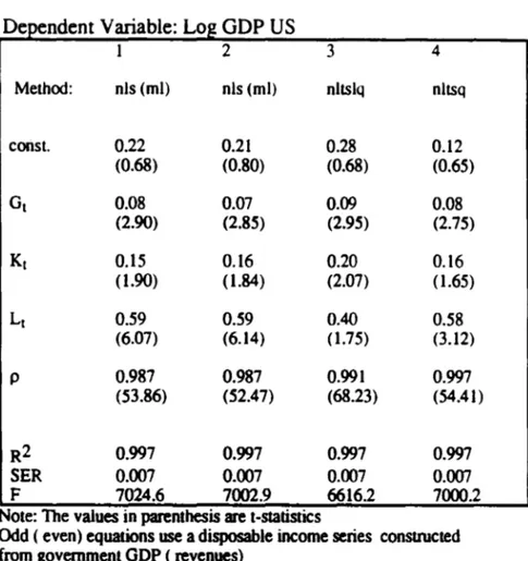
TABLE V Time Series Estimations Dependem Variable: Log GDP US
1 2 3 4 Method: nls (ml) nls (ml) nltslq nltsq conSl. 0.22 0.21 0.28 0.12 (0.68) (0.80) (0.68) (0.65) Gt 0.08 0.07 0.09 0.08 (2.90) (2.85) (2.95) (2.75) Kt 0.15 0.16 0.20 0.16 (1.90) (1.84) (2.07) ( 1.65) Lt 0.59 0.59 0.40 0.58 (6.07) (6.14) (1.75) (3.12) P 0.987 0.987 0.991 0.997 (53.86) (52.47) (68.23) (54.41) R2 0.997 0.997 0.997 0.997 SER 0.007 0.007 0.007 0.007 F 7024.6 7002.9 6616.2 7000.2
Note: The values in parenthesis are t-statistics
Odd ( even) equations use a disposable income series constructed from govemmenl GDP (revenues)
In all the estimations lhe effect of govemment expenditures over GDP ranges from seven percentage points to nine points. This is well below lhe estimates in Aschauer (1989a) lhat obtained values around 0.35. We can give some altemative explanations for lhese discrepancies. First. he works in a partial equilibrium framework where lhe effect of tax collection and lhe law of motion of private capital, as well as lhe determinams of labor supply, are not taken into account ( only a production function is estimated). In lhis case. simultaneity problems are likely to arise and labor and capital may be correlated with lhe disturbance to lhe production function. and lhis would bias lhe estimates of lhe coefficient of lhese variables. Second. ali variables in his equations are in leveis, which is a classical case of spurious regression. In lhis case, the results are influenced by lhe common trend between independent and dependent variables. Third, we are using a different data set: Aschauer (1989a) uses lhe stock of govemment structures arid we use expenditures in structures and durables ( and ours is a quarterly data set and his is annual). This was shown to reduce lhe coefficient in a similar way in section 4 of lhis paper.
In any case, even our results, with the govemment coefficient between 0.07 and 0.09, imply a significant role for public infrastructure. It means that the effect of government capital expenditures on production is around one quaner of the effect of private capital and that the public investment elasticity of output is around ten per cent, and always significant.
Regressions number 1 and 2 use a technique that is closest to the one used by Benhabib and Jovanovic. although we have a different error structure. They use Maximum Likelihood technique and we use Non Linear Least Squares. which is asymptotically equivalent to ML if the residuais are assumed to follow the normal distribution. The value we got for the coefficient of capital is smaller than what is in generally assumed (one third ) and it implies. together with a labor coefficient around 0.60, at least in this short run data set, that the coefficient of social capital is negative. However, the higher standard deviation of the capital coefficient estimates does not allow us to conclude with cenainty that 8 is not positive. This is true for all regressions in Table three and it dramatizes the results Benhabib and Jovanovic (1991) obtained for time series data. This paper obtained values for 8 which are either toe low to be compatible with gr~wth or are not significant. Finally, the value p • 0.99. is in line with the rest of the literature, implying high persistence of technological shocks.
Regressions 3 and 4 use nonlinear two stage least squares with labor lagged one period employed as instrument. They should be considered the main estimate of the model. The results are very close to the nonlinear least square estimates, only differing in that the capital coefficient in equation (3) is slightly higher while labor coefficient is much smaUer than the usual estimates in the literature. Equation (4) almost reproduces equation (2): a significant and relative high coefficient for govemment investments, a labor coefficient eS,timate slightly smaller than expected and a capital coefficient incompatible with endogenous growth ( although, once again. the high standard error does not give us a lot of confidence in this estimate).
A common objection to this kind of exercise is that govemment capital would not be qualitatively different from private capital. Hence, the estimated coefficients are misleading in that
cp
does not measure the specific impact of public capital but the impact of any capital in general. Ot would merely crowd out Kt. We tested this hypothesis running restricted equations where we assumed thatcp
is equal to the private capital coefficient. The results reject the hypothesis thatcp=a+8.
The F-statisúcs are 0.063 and 2.582 for the case where t is measured as Oovernment ODP/ODP or Oovemment revenues/ODP, respectively, and with degrees of freedom 1 and 70 are not significant at the 5% leveI.In the regression presented below we made explicit the proper restrictions on the coefficients of the variables in equation five. In other worlds. we assumed. before estimating, that the labor coefficient is (1-
a )
and that the capital coefficient is (a
+e ).
We used nonlinear two stage least squares with labor lagged one period as the instrument.
Constarit
q,
a
e
p
Yt 0.02 0.08 0.41 - 0.25 0.989
(0.65) (2.75) (2.20) (-1.56) (54.24) R2 = 0.997, SER = 0.007, F = 7000.2
Although the total coefficient of capital approximately sums to the same value as in table V ( Le., a+e
=
0.16) we can see now thate
not only is not significant at the 5% leveI but has the wrong signo All other coefficients remain more or less the same, and the public investment elasticity is relatively high and significant.In order to double check these results and obtain an independent estimate of the parameter
q,
of productive public expenditures we estimate an equation using a series for physical capital from the Bureau of Economic Analysis data set. In other words, we substituted (1-tt)Y t-l for capital stock in the final form of lhe model. We employed threealternatives estimation methods: two stage least squares ( labor is endogenous and lagged labor is the instrument), ordinary least squares and non-linear least squares. In the two stage and the ordinary least square we also used the Cochrane-Orcutt method to correct for autocorrelation and to identify the parameter p. The results for model I are presented in table VI below.
TABLE VI
Estimations with Physical Capital
2 3 Method: LS NLS (rnl) TSLQ consto -0.63 0.13 -0.03 (0.68) (0.76) (-0.02) GI 0.10 0.10 0.09 (4.02) (3.77) (3.41) KI 0.25 0.25 0.20 (7.8) (4.05) (2.11) LI 0.79 0.81 0.88 (5.62) (7.8) (5.03) p 0.73 0.73 0.68 (7.1) (7.1) (7.47) R2 0.997 0.997 0.997 F 4841.9 5286.0 5223.5 SER 0.008 0.007 0.007
Note: The values in parenthesis are t-stalistics
The estimates from these regressions are close to the previous results. The coefficient of Gt remains close to 0.10 and is highly significant, confirming that productive public expenditures do play ao important role in determining the movements of Y t. On the other haod the results do not suppon the hypothesis of externaI effects from physical capital: the coefficient 9 stays between 0.08 and 0.05, so that a+9 is far from one (it ranges from 0.25 to 0.20). The values of the correlation parameter p however are lower than the ones we got in the previous estimations although the techniques in estimations (1) aod (3) are different. On average, the estimates using physical capital are fairly consistent with the outcomes from the complete model.
S.b Total Factor Productivity
Following the steps of section 4.b we estimated the impact of public capital on the leveI and growth rates of total factor productivity. The results of this section, especially column 2 at table V below, have interesting consequences for the debate about the slowdown of productivity growth. They point to the fact that at least part of this deceleration may be traced to the slowdown in government investment between 1970 aod 1990: in our estimates a 10% decrease in the rate of growth of public investment causes ao 1 % decrease in the rate of growth of total factor productivity.
We estimated equations (11) and (12) to measure the impact of public investment on productivity and productivity growth. The results are presented in table five below.
Table VII TFP:Time Series Data
2 Ft DFt consto 0.94 0.003 (8.47) (0.40) Gt 0.11 (4.26) DGt 0.09 (3.33) p 0.83 (11.09) R2 0.85 0.14 SER 0.007 0.007 F 178.0 11.2
Ft: logY - 0.75*logL - 0.2S*logK
Column 1 presents the estimate of equation 11. We used the Cochrane-Orcutt technique as the residual" is assumed to be autocorrelated. The estimate of the coefficient of govemment investment is significant and positive, it has values close to those in Table IH: the elasticity of total factor productivity is around 0.10. The persistence factor is positive and significant at the 5% leveI. In coIumn two we regress total factor productivity growth on public investment growth. The elasticity coefficient in this case is 0.09 and significant at the 5% leveI. Not surprisingly, the R-square and F statistics falI considerably when we switched from leveI to growth rate estimations.
It is well documented that in the period under consideration public investment did not keep pace with GDP growth. Public investment, measured as the sum of structure and equipment purchases, as a proportion of GNP, falls from 3.1 % in 1972 to 2.1 % in 1983, while the proponion for expenditures on structure alone falIs from 2.6% to 1.5% in the same period. The resuIts in Table VII match Aschauer (1989a) and Morrison and Schwartz (1992), as they alI suggest that this phenomenon may have had a negative impact over productivity growth, which grew at an average annual rate of 2% from 1950 to 1970 but only 0.8% from 1971 to 1985.
6 Conclusion
We presented in this paper three sets of regressions with the objective of estimating the impact of public investment and infrastructure capital on economic growth. In all of them the impact of the public sector is significant, whelher we use investment or capital series. The estimates of lhe oUlput elasticity to public investment range from a 0.07 for U .S. data to 0.3 for lhe growlh accounting regressions when we used lhe public capital measure we created. This discrepancy is not entirely surprising given the vast differences in the frameworks used. However. within each particular framework lhe coefficient of public capital or public investment is fairly robust.
Funhermore. the data also suppons the hypolhesis lhat total factor productivity growlh is directly affected by lhe growth of public capital. This result has imponant policy implications as a decline in the rate of growth of public investment in infrastructure may help to explain disparities in growth rates across countries or lhe slowdown of productivity growlh of a single nation.
We found lhe overall results very encouraging for upholding lhe hypolhesis of lhe productive impact of public expenditures in growth models. The hypothesis of the externaI effect of capital, however, is only weakly supponed by the cross-country data and not supponed at ali by lhe time series data, a result that is similar to both Romer (1987) and Benhabib and Jovanovic (1991). Moreover in lhe growth accounting framework, allhough lhe estimates of lhe log difference of total capital is larger lhan lhe capital share it is well below lhe necessary values for endogenous growlh.
Appendix: The Data
Cross Section Data
Data for GDP and labor force were taken from Summers and Heston World Table. The fact lhat lhe labor series is a labor force series and not a measure of ·actual hours worked is problematic because it does not capture variations in lhe use of lhe labor input. This especially affects lhe growlh accounting estimations in Section 2 but it may also harm lhe cross section estimates in Section IV if lhe proportion of actuallabor used to labor force varies toa much among different countries.
Data for govemment capital expenditure and two altematives series for
governrnent expenditures ("Central Govemment Expenditures Plus Borrowing Minus Lending" and "General Govemment Expenditures") were taken from IMF's
"Intemational FinanciaI Statistics".
Although the Summers and Heston data set goes untilI988 we used the 1986 data for cross-section estimations ( Section four) because there are toa many missing observations for 1987 and 1988 in it. Our data set includes most countries from Europe. North and South America. twelve nations from Africa and thirteen from Asia and Oceania. We did include Oil Exporters countries although in some regressions we excluded Kuwait which is an extreme outlier. The reason for having only 67
observations is that the "Govemment Capital Expenditures" series from the IFS cover a smaller number of countries than the Summers and Heston data-set.
We used altematives series for (l-tt-I>Yt-l variable. We employed both "Central Govemment Expenditures Plus Borrowing Minus Lending" and "General Govemment Expenditures" (both from the IFS) divided by GDP as proxies for t. We also tried different lags. We did this because. as physical capital is a function of past variables and assumed to complete depreciate. we were not sure which would be the correct interpretation of "t-I" in the variable (I-tt-})Y l-I.
We used series for 1975 and 1980. 1975 is the frrst year we have enough observations so that the regression in this case use both ends of the data set (1975 and
1986). Both 1975 and 1980 are reasonable spans for the total depreciation hypothesis and the more appropriate series to study low-frequencies movements that we are concemed with in this paper ..
Finally, Section 2 and some regressions of Section 4 used a public capital series constructed with data from various data sets. The methodology is explained below.
At any period (public) capital is given by: t-l
Kgt
= (
1 -ô ) t Kgo +L (
1 -ô ) i Igt-l-ii=O
where Kg is public capital, Ig public investment and Ô the depreciation rate. Hence, in order to obtain the public capital series we need an investment series and estimations of public capital in period zero and of the depreciation rate.
We used gross investment from the IMF's Intemational FinanciaI Statistics as our investment series. For initial capital we flfst estimate the average ratio of public
investment (from IFS tables again) to total investment (from the Summers and Heston world tables). We averaged both series over 1973 to 1988, the years we have data from
the IFS tables. We hypothesized that on average the ratio of public to total investment is a good approximation of the ratio of public to total capital. We then multiplied the value for 1972 ( total) capital stock from Benhabib and Spiegel ( 1992a) by this ratio. The result was the stock of public capital at the initial period. Note that Benhabib and Spiegel (1992a) used lhe Summers and Heston investment series to construCl their capital series, and thal series is a total investment series ( private plus public), so that the product of total capital by the ratio of public to total capital give us the public capital series:
Ig Kg
T·
KTo=KT .KTo= KgoIn the expression above KT is total capital, and the ratios are averages. Ideally we would like to have a ratio of capitaIs and not investments but in this case, of course, we would not need to estimate KgO. We also would like to have an estimation that would begin long before the fust date ( 1975 in the present case) of our regressions, in order to make its effect in the final estimates as weak as possible. This however was not possible because the IFS series starts in 1973 and we felt it would be quite arbitrary to use this ratio to multiply total capital values far before this date. The series of private capital used in Section 2 is merely the difference between total capital and public capital.
Time Series Data
AlI the data in the time series were obtained from the Citibase data set, with the exception of a capital series from the Bureau of Economic Analysis data set.
In this set of regressions we used total hours worked from the Household Survey for labor and Gross Domestic Product for income. There is no quanerly data for the stock of public structure or durable goods, so we used total expenditures in structure and durables of the general govemments. Here we simply added four series: total expenditure in sttucture for central govemment, total expenditure in structures for state and local govemment, expenditures in durables for central govemment and expenditures in durables for state and local govemments.
We constructed two altemative series for disposable income «(l-tJYt). For the frrst one t was constructed as "Federal Govemment ReceiptslGDP" and in the other it was constructed as "Govemment GDPrrotal GDP". Given that in the model taxes are the only way that govemment can fmance its expenditures both series are theoretically equivalent. AlI the variables are seasonally adjusted and in 1982 US dolIars.
References
Aschauer. D .• (1989a) "Is Public Expenditure Productive?" Journal of Monetary
Eco1lomics. 23, March. pp. 177-200.
Aschauer. D., (1989b) "Public Invesunent and Productivity Growth in the Group of Seven." Economic Perspectives. 13. no. 5, pp 17-25.
Barro. R. J .• (1990) "Govemment spending in a simple Model of Endogenous Growth,"
Journal of Polítical Economy, 98. pp. S 103-25.
_ _ _ , (1991) "Economic Growth in a Cross Section of Countries. " Quarterly Journal
of Economics, 106. May, pp. 407-43.
_ _ _ o and X. Sala-i-Martin. (1992a) "Public Finance in Models of Economic Growth,"
Review of Economic Studies.
Benhabib.1. and B. Jovanovic. (1991) "Extemalities and Growth Accounting." American
Economic Review. 81, pp. 82-113
_ _ ~_. and M.M. Spiegel (1992a) "The Role of Human Capital And Political lnstability in Economic Development." Manuscript. New York University.
and (1992b) "The Role of Human Capital in Economic Development: Evidence from Aggregate Cross-Country and Regional US Data." Manuscript. New York University.
Christiano. L.J. (1987) "Comment on Romer's 'Crazy Explanations of The Productivity Slowdown'," Manuscript. Federal Reserve Bank of Minneapolis.
Holtz-Eakin. D., (1989) "The Spillover Effects Of State-Local Capital." Manuscript. Columbia University.
Holtz-Eakin. D .• (1992) "Public-Sector Capital and Productivity Puzzle", NBER Working Paper No. 4122
Hulten. C and R. Schwab. (1984) "Regional Productivity Growth in USo Manufacturing:
1951-1978," American Economic Review, 74, pp. 152-162.
lntemational Monetary Fund.lnternational Financiai Statistics Yearbook. various issues. Levine, R. and Renelt, (1992) "A Sensitivity Analysis Of Cross-County Growth
Regressions," American Economic Review, 82, September, pp. 942-63
Lucas, R., (1988), "On the Mechanics of Economic Development," Joumal of Monetary Economics, 22, pp. 3-42.
Mankiw, G., Romer, D. and D. WeH, (1990) "A Contribution to the Empirics of Economics Growth" NBER working paper No. 3541
Morrison. C. J. and A.E. Schwartz (1992) "State lnfrastructure and Productive Perfonnance." NBER working paper No. 3981.
Munnel, A.H., (1990a) "Why has Produetivity Growth Deelined? Produetivity and Publie Investment," New England Economic Review, January, pp. 3·22.
Munnel, A.H., (1990b) "How Does Publie Infrastrueture Affeet Regional Eeonomic Performance," New EIlglalld Economic Review, September, pp 11·32.
Nadiri, M.1. and T.P. Manuneas (1992) "The Effects of Publie Infrastrueture and R&D Capital on the Cost Strueture And Perfonnance of US Manufacturing Industries," Manuscript, New York University.
Rebelo, S., (1991) Long Run Policy Analysis and Long Run Growth," Journal of
Polítical Economy, 98, pp. S
Romer, P (1987) "Crazy Explanations for The Productivity Slowdown," NBER Macroeconomics Annual, 1987, 1, pp. 163·201.
_ _ _ , (1989) "Capital Aeeumulation in the Theory of Long·Run Growth," in R. J. Barro (ed.) "Modern Business Cycle Theory," Harvard University Press.
Summers, R. and Alan Heston (1991) "The Penn World Table: An Expanded Set of Intemational Comparisons" 1950·1988," Quanerly Journal of Economics, 106,
May, pp. 327·368.
ENSAIOS ECONÔMICOS DA EPGE
100. JUROS, PREÇOS E DÍVIDA PÚBUCA - VOL. I: ASPECTOS TEÓRICOS - Marco Antonio C. Mat1ins e Clovis de Faro - 1987 (esgotado)
101. JUROS, PREÇOS E DÍVIDA PÚBUCA VOL. ll: A ECONOMIA BRASILEIRA 1971/85
-Antonio Salazar P. Brandão, Marco Antonio C. Martins c Clovis de Faro -1987 (esgotado) 102. MACROECONOMIA KALECKlANA - Rubens Penha Cysne - 1987 (esgotado)
103. O PREÇO DO DÓLAKNO MERCADO PARALELO, O SUBFATURAMENTO DE EXPORTAÇÕES E O SUBFATIJRAMENTO DE IMPORTAÇÕES - Fernando de Holanda Barbosa, Rubens Penha Cymc c Marcos Costa Holanda - 1987 (esgotado)
104. BRASn.IAN E.XPERIENCE wrIH EXTERNAL DEBT ANO PROSPECTS FOR GROwm -Fcmando de HoImda BaIbou anel Maauel SandlCI de La CaI-1987 (esgotado)
lOS. KEYNES NA SEDIÇÃO DA ESCOlJIA PÚBUCA - Amonio Maria da Silveira - 1987
(cagotado)
106. O TEOREMA DE FROBENIU8-PERRON -Carlos Ivan SimoaIcn LcIl- 1987 (esgotado) 107. POPULAçÃO BRASILEIRA -JCIIé Moatclo -1987 (esgotado)
108. MACROECONOMIA - cAPÍTIJLO VI: "DEMANDA POR MOEDA E A CURVA LM" -,
Mario Hcmiquc Simonscn c Rubens Penha Cymc - 1987 (esgotado)
109. MACROECONOMIA -
cAPÍTIJLo vn:
"DEMANDA AGREGADA E 'A CURVAIS" -MarioHcmiquc SimonIen c Rubens Penha Cymc -1987 (esgotado)
110. MACROECONOMIA MODELOS DE EQUILÍBRIO AGREGATIVO A CURTO PRAZO
-Mario Henrique SÍIIlODICIl c Rubens Penha Cymc -1987 (esgotado)
111. TIIE BAYESIAN FOUNDATIONS OF SOLUTIONS CONCEPTS OF GAMES - Sérgio
Ribeiro da Costa WcrIaDg c Tommy Cbin-Chiu Tan - 1987 (esgotado)
112. PREÇOS ÚQUIDOS (PREÇOS DE VALOR ADICIONADO) E SEUS DETERMINANTES; DE PRODUTOS SELECIONADOS, NO PERÍODO 1980/10
SEMESTRFl1986 - Raul
Ekcrmm - 1987 (esgotado)
113. EMPRÉSTIMOS BANCÁRIOS E SALDO-MÉDIO: O CASO DE PRESTAÇÕES - Clovis de Faro - 1988 (esgotado)
114. A DINÂMICA DA INFLAÇÃO - Mario Henrique SimoDscn - 1988 (esgotado) ,
115. UNCERTAIN1Y AVERSIONS ANO TIIE OP'IMAL CHOISE OF PORTFOUO - Jamcs Dow
c Sérgio Ribeiro da Costa W crtang -1998 (esgotado)
117. FOREIGN CAPITAL ANO ECONOMIC GROWTH 1lIE BRASD.lAN CASE STIJDY -Mario Henrique Simonsen - 1988 (eagotado)
118. COMMON KNOWLEOOE - Sérgio Ribeiro da Costa WcrlaDg - 1988 (eagotado)
119. OS FUNDAMENTOS DA ANÁlJSE MACROECONÔMICA - Mario Hcmiquc Simonsen e
Rubens Penha Cysne - 1988 (esgotado)
120. CAPÍ11JLo
xn -
EXPECTATIVAS RACIONAIS - Mario Henrique Simcmsen - 1988 (esgotado)121. A OFERTA AGREGADA E O MERCADO DE TRABALHO - Mario Henrique SimODSCll e
Rubens Penha Cysne - 1988 (esgotado)
122. INÉRCIA INFLACIONÁRIA E INFLAÇÃO INERCIAL - Mario Henrique Simcmsen - 1988 (eagotado)
123. MODELOS DO HOMEM: ECONOMIA E ADMINISTRAÇÃO - Antoaio Maria da SiMira -1988 (esgotado)
124. UNDERINVOINCING OF EXPORTS, OVERINVOINClNG OF IMPORTS, ANO 1lIE DOlLAR PREMIUN ON
nm
BLACK MARKET - Fernando de Holanda Barbosa, RubeDsPcaba Cymc e Marcos Costa Holanda -1988 (eagotado)
12S. O REINO MÁGICO DO CHOQUE HETERODOXO - Femando de Holanda Barbosa, Antonio SaIazIr Peaoa Brandio e CkMs de Faro - 1988 (eagotado)
126. PLANO CRUZADO: CONCEPÇÃO E O ERRO DE POúnCA FISCAL - R.ubcna Penha
Cymc - 1988 (eagotado)
127. TAXA DE JUROS FL1ITUANTE VERSUS CORREÇÃO MONETÁRIA DAS PRESTAÇÕES: UMA COMPARAÇÃO NO CASO DO SAC E INFLAÇÃO CONSTANTE -Clovis de Faro -1988 (esgotado)
128.
cAPÍTULO n -
MONETARY CORRECTlON ANO REAL INTEREST ACCOUNTING -Rubens Penhacysnc -
1988 (esgotado)129. CAPÍTIJLO
m -
INCOME ANO DEMAND POliCIES IN BRAZIL - Rubens Penha Cysne-1988 (esgotado)
130. CAPÍTIJLO IV BRAZILIAN ECONOMY IN 1lIE EIGlITIES ANO 1lIE DEBT CRISIS
-Rubens Penha Cyme -1988 (eagotado)
131. 1lIE BRAZILIAN AGRICUL TIJRAL POliCY EXPERIENCE: RATIONALE ANO FUTURE DIRECTlONS -Antonio SaIazar Pessoa BrandIo - 1988 (esgotado)
132. MORATÓRIA INTERNA, DÍVIDA PÚBUCA E JUROS REAIS - Maria Silvia Bastos
Marques e Sérgio Ribeiro da Costa Wcrlang -1988 (eagotado)
133. CAPÍ11JLo IX - TEORIA DO CRESCIMENTO ECONÔMICO - Mario Henrique Simonscn -1988 (eagotado)
134. CONGELAMENTO COM ABONO SALARIAL GERANDO EXCESSO DE DEMANDA -Joaquim Vieira Ferreira Levy e Sérgio Ribeiro ,da Costa WcrIang - 1988 (esgotado)
135. AS ORIGENS E CONSEQUÊNCIAS DA INFLAçÃO NA AMÉRICA LATINA - Fernando de
Holanda Barbosa - 1988 (esgotado)
136. A CONT A-CORRENfE DO GOVERNO - 1970/1988 - Mario Hcmiquc SimOJllCll - 1989 (esgotado)
137. A REVIEW ON
nm
nmORY OF COMMOW KNOWLEDGE - Sérgio Ribeiro da CostaWcrIang - 1989 (esgotado)
138. MACROECONOMIA - Fernando de Holanda Barbosa - 1989 (esgotado)
139. TEORIA DO BALANÇO DE P'AGAMENTOS: UMA ABORDAGEM SIMPLIFICADA - João Luiz TcmCÍlo BamJ80 -1989 (cagotado)
140. CONT ABll..IDADE COM JUROS REAIS -Rubc:m Penha Cyanc - 1989 (esgotado)
141. CREDIT RATIONING AND
nm
PERMANENT INCOME HYPOlHESIS - VicenteMadrigaI, Tommy Taa, n.aiel Vicent, Sérgio Ribeiro da CoIta Wedq - 1989 (esgotado) 142. A AMAZÔNIA BRASILEIRA -Ney Coe de 0IMira -1989 (esgotado)
143. DESÁGIO DAS LFrs E A PROBABll..IDADE IMPÚCITA DE MORATÓRIA - Maria Silvia
Butos Marques e Sérgio Ribeiro da Costa WcrIaog - 1989 (esgotado)
144.
nm
LDC DEBT PROBLEM: A GAME-THEORETICAL ANAUSYS - Mario HcoriqueSimonscn e Sérgio Ribeiro da Costa WcdaDg - 1989 (esgotado)
145. ANÁliSE CONVEXA NO Rn -Mario Hemique SimoDIcn - 1989 (esgotado)
146. A CONI'RoVÉRSIA MONETARISTA NO HEMISFÉRIO NORTE - Fernando de Holanda Barbosa - 1989 ( esgotado)
147. FISCAL REFORM AND STABn.IZATION: lHE BRAZILIAN EXPERIENCE - Fernando de
Holanda Barbosa, Antonio SaJaDr Pessoa Brandão e Clovis de Faro - 1989 (esgotado)
148. RETORNOS EM EDUCAÇÃO NO BRASIL: 1976/1986 - Carlos Ivan Simonscn Leal e Sérgio
Ribeiro da Costa Wcrlang,- 1989 (esgotado)
149. PREFERENCES, COMMON KNOWLEDGE AND SPECULATIVE TRADE - Jamcs Dow,
Vicente Madrigal c Sérgio Ribeiro da Costa WcrIang - 1990 (esgotado)
150. EDUCAÇÃO E DISTRIBUIÇÃO DE RENDA - Carlos Ivan Simonscn Leal e Sérgio Ribeiro da
Costa WcrIang - 1990 (esgotado)
151. OBSERVAÇÕES A MARGEM DO TRABALHO" A AMAZÔNIA BRASILEIRA" - Ney Coe de Oliveira -1990 (esgotado)
152. PLANO COlLOR: UM GOLPE DE MESTRE CONTRA A INFLAÇÃO? - Fernando de Holanda Barbosa - 1990 (esgotado)