(Annals of the Brazilian Academy of Sciences)
Printed version ISSN 0001-3765 / Online version ISSN 1678-2690 www.scielo.br/aabc
Electromagnetic fields at the sea bottom induced by a line of immersed electric dipoles
EDSON E.S. SAMPAIO
CPGG, Instituto de Geociências, Universidade Federal da Bahia, # 213-B, Campus Universitário de Ondina, 40170-290 Salvador, BA, Brasil
Manuscript received on June 19, 2009; accepted for publication on December 1, 2010
ABSTRACT
The analysis of electromagnetic fields caused by alternate or transient electric currents flowing along a cable in sea water has several applications. It supports the interpretation of electromagnetic geophysical data and safety procedures against the threat of sea mines. The approach to the problem employs a magnetic vector potential in the frequency domain due to a pulse source electric dipole, and performs Laplace and Hankel transforms and integration along the cable, to describe the variation of the magnetic induction field due to an electric dipole of finite length. The result is applicable to shallow or deep sea water environments, adaptable to any transmitting current waveform and useful for wave-field separation. The prospects relate to a horizontal receiving coil at the sea bottom and simulate: a minesweeper campaign with a current source at the sea surface or a geophysical survey with a current source close to the sea floor. Therefore, the present analysis may serve: to define parameters in counter-sweeping of submarine mines; to map the conductivity of sediments under shallow waters for the prevention and control of contamination; and as a first approach in the characterization of offshore mineral and oil economic deposits.
Key words: dipoles, electromagnetic energy, induced fields, sea.
INTRODUCTION
Magnetic tail is a nautical designation for a line of electric dipoles. It consists of a steady state or a transient electric current flowing along a cable of finite length. The tail may be placed at any point between the surface and the bottom of a salty water layer to originate an electromagnetic field. The description of the magnetic field vector in the time domain caused by the tail inside the same region is useful for several applications in physics and in electrical and mechanical engineering to calibrate laboratory simulations and field experiments.
In naval engineering, it is employed to protect ships from the threat of sea mines, for the safety of maritime transportation (Pinheiro and Sampaio 1993, Rayner 2007). In geophysics, it can be of help
in investigating the submarine substratum (Constable and Cox 1996, Flosadóttir and Constable 1996, Goldman 1990); to map pollution of the sea bottom in shallow waters (Cheesman et al. 1987, Scholl and Edwards 2007, Souza and Sampaio 2001); to prospect for minerals in the seafloor (Wolfgram et al. 1986, Wynn 1988); and to detect the presence of gas hydrate deposits (Edwards 1997). It is also becoming increasingly important for the prospection and monitoring of offshore hydrocarbon reservoirs (Ellingsrud et al. 2002, Eidesmo et al. 2002).
We compute and analyze in this paper both the spatial and the time variation of the vertical component of the magnetic field due to a magnetic tail for two cases: (1) a current source at the sea surface and a horizontal coil at the sea bottom; and (2) a current source and a horizontal coil at the sea bottom. The first case simulates the situation of a minesweeper campaign and may have application for monitoring pollution in shallow sea waters. The second case simulates a submarine geophysical investigation.
There is a substantial body of geophysical investigation about electromagnetic sources on the sea surface and in the sea floor, as for example: (Chave and Cox 1982, Chave et al. 1991, Constable 2006, Constable and Weiss 2006, Løseth and Ursin 2007, Guimarães and Sampaio 2008a, b). However, this paper has two distinct goals and employs a different procedure from these investigations.
The goals of this paper are: (1) to provide a general solution of the problem, which is valid for any current waveform; and (2) to represent the main part of the wave field as a series of real terms identified with successive reflections at the top and the bottom of a sea water layer confined between the air and a homogeneous substratum. This one-dimensional model represents a new procedure applicable in marine transportation safety and for mapping seafloor pollution of marshes and bays in shallow waters. Though it has a restricted application in geophysics, especially in reservoir characterization, the analysis of 2-D and 3-D scattering problems usually employs the result of a one-dimensional model in building up the respective 2-D or 3-D solutions. Such is the case, for instance, of the Sampaio approximation (Sampaio and Fokkema 1992, Sampaio and Popov 1997, Batista and Sampaio 2003), as well as of the Born or integral equation approximations (Wannamaker et al. 1984, Torres-Verdín and Bostick Jr. 1992, Spies and Habashy 1995, Torres-Verdín and Habashy 2001, Tseng et al. 2003). Furthermore, the contribution of a homogeneous or a layered half-space is usually larger than the contribution scattered by 2-D or 3-D inhomogeneities. So, it is necessary to understand better the homogeneous or 1-D response in order to interpret adequately the inhomogeneity response.
DEVELOPMENT OF THE SOLUTION
We will develop the algebra of the solution in this section. However, we will not reproduce here the basic details of the mathematical development of this problem because its theory is well known in the geophysical literature (Stratton 1941, Wait 1982, Ward and Hohmann 1988, Pinheiro and Sampaio 1993).
DIPOLE IN ACONDUCTIVEINFINITEMEDIUM
Let an electric dipole be in a conductive infinite medium as shown in Figure 1. The magnetic vector poten-tial,A(x,y,z, ω), and the magnetic induction field,B(x,y,z, ω), are related by the following equation:
B= ∇ ×A, (1)
where: (x,y,z) represent the coordinates of the observation point,ω=2πf, and f is the frequency.
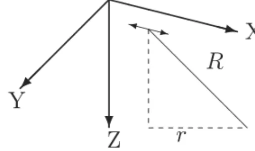
X
Z
Y
r
R
Fig. 1 – Ax-directed electric dipoleI d x0iat (x0,y0,z0) in a homogeneous isotropic and infinite medium. Observation point
at (x,y,z). R represents the source-receiver distance, andr the horizontal projection ofR.
The magnetic vector potential obeys the non-homogeneous Helmholtz wave equation:
∇2A+κ2A= −μ0Js. (2)
In Equation 2, the wave-number κ = pμ0ǫω2−iμ0σ ω, where: i = √−1, μ0 = 4π10−7(henry/m)
is the magnetic permeability of the free-space,ǫ is the dielectric permittivity, andσ is the electric
con-ductivity. In free space,κ0 = √μ0ǫ0ω. The term that represents the source is the Fourier transform of
the current density waveform, Js. We define an oscillating electric dipole at (x0,y0,z0), as represented in Figure 1, by the following expression:
Js = I(ω)d x0δ(x −x0) δ(y−y0) δ(z−z0)i. (3)
In Equation 3, I(ω) represents the Fourier transform of the electric current; d x0 is the element of length
of thex-oriented electric dipole, and eachδ(φ−φ0) represents the Dirac delta function with singularity
onφ = φ0. Equation 2 shows that the primary potential, Ap(x,y,z, ω), presents only an x-component, and it is given by:
Ap(R, ω)=
μ0I(ω)d x0
4π
e−iκR
R i, (4)
where: R = p(x −x0)2+(y−y0)2+(z−z0)2 is the source-receiver distance. Because R is always
positive, we guarantee the convergence of the potential at infinity, assuming thatℑ(κ) < 0. Applying
We obtain the solution for an arbitrary function of the current waveform by convolving this function with the impulse response solution. So, we solve the problem expressing the source current waveform as: I(t) = Cδ(t)ampere and I(ω) = Ccoulomb. We also assume the quasi-static condition, valid
for frequencies below 1MHz, and a non-magnetic medium. Soσ >> ǫω, and we may write either κ ≈
√
2
2 √μ0σ ω (1−i) or κ ≈
√
−μ0σs, s = iω. Next, we employ Laplace Transform in Equation 4
to obtain the primary potential and the magnetic field in the time domain due to a dipole in a conductive infinite medium.
ap(R,t)=F(R,t)i, (5)
bp(R,t)=
μ0σ
2t F(R,t)
0i,−(z−z0)j, (y−y0)k, (6)
F(R,t)=
q
μ30σ Cd x0
8√π3
e−μ0σ4tR2
√
t3 u(t),
whereu(t) is the Heaviside step function,u(t)=0 fort <0 andu(t)=1 fort >0.
DIPOLE IN ATHREE-LAYEREDMEDIUM
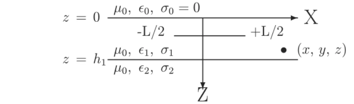
Figure 2 illustrates the geometry of the model. In the air, z < 0, μ0, ǫ0 ≈ 10−9/(36π )(farad/m), and σ0 = 0. In the sea, 0 < z < h1, μ1 = μ0, ǫ1 = 81ǫ0, and 1 (S/m)< σ1 < 6 (S/m). In the substratum, z>h1, μ2=μ0, ǫ0< ǫ2<25ǫ0, and 10−3(S/m)< σ2<10−1(S/m).
μ
0, ǫ
0, σ
0= 0
μ
0, ǫ
1, σ
1μ
0, ǫ
2, σ
2z
= 0
z
=
h
1-L/2
+L/2
•
(
x, y, z
)
X
Z
Fig. 2 – Illustration of the geometry of the problem with a magnetic tail positioned inside a salty water layer, centered at
y0=0, 0≤ z0 ≤h1 and laid between−L/2≤ x0≤ +L/2. Observation point at (x, y,z) of a homogeneous and isotropic
three-layered medium.
The secondary potential obeys the homogeneous wave equation and has both thex and thez
compo-nent for the geometry illustrated in Figure 2. Therefore, forη= x,z and j =0,1,2 its general solution
can be expressed by the following series of Hankels’ integrals:
Aη,Sj(x,y,z, ω) =
∞
X
n=0
cos(nφ) Z ∞
0
Fη,±je±αj|z−z0|J
n(λr)dλd x0, (7)
where: cos(φ) = (x−x0)
r andαj =
q
λ2−κ2j is complex with a positive real part. Employing Hankel transform (Sommerfeld 1949), Equation 4 assumes the following expression for the dipole in the water layer:
Ap,1(x,y,z, ω)=
μ0I(ω)
4π
Z ∞
0 λ α1e
In Equations 7 and 8, Jn(λr) represents the Bessel Function of first kind andnth order and
r =p(x −x0)2+(y−y0)2.
Adding the secondary and the primary potentials expressed by Equations 7 and 8, respectively, yields the total potential in the three-layered medium. The solution for the eight functionsFη,±j(λ) is determined
by applying the condition of convergence of the potentials at infinity, Maxwell’s equations, Equation 1, and the following boundary conditions:
Bz,0=Bz,1; μ1Bx,0=μ0Bx,1; onz=0, Ey,0 =Ey,1; μ1By,0=μ0By,1; onz=0, Bz,1=Bz,2; μ2Bx,1=μ1Bx,2; onz=h1, Ey,1= Ey,2; μ2By,1=μ1By,1; onz=h1.
(9)
THETAIL INTHREE-LAYEREDMEDIA
We represented the tail by a horizontal line of electric dipoles of length L. Figure 2 illustrates both the
geometry of the model and the magnetic tail in the sea. By applying the boundary conditions expressed in the system of Equations 9 and integrating along the cable length (x0), one writes the final expression for Bz,1(R, ω) due to a magnetic tail situated between the surface and the sea floor.
Bz,1(R, ω) = − μ0
4π I(ω) ∂ ∂y
Z ∞
0
λ α1e
−α1|z−z0|+F+
x,1(λ)e+α1z
+Fx−,1(λ)e−α1z
Z +L2
−L
2
J0(λr)d x0
dλ
, (10)
Fx+,1 = λ α1
R1,2e−2α1h1(R1,0e−α1z0 +e+α1z0)
1−R1,0R1,2e−2α1h1 ,
Fx−,1 = λ
α1
R1,0(R1,2e+α1z0e−2α1h1 +e−α1z0)
1−R1,0R1,2e−2α1h1 ,
R1,j =
α1−αj
α1+αj
, j=0,2.
The magnetic field in the time domain
To obtainbz,1(R,t), we apply Fourier or Laplace transform to Equation 10. Only in special casesbz,1(R,t)
is obtained analytically, becauseαj, j = 1,2,3 is also a function ofω. In general, it is necessary to perform three numerical integrations: inλ, x0, and ω. Therefore, the computation of the time domain
bzs(R,t). So, we will have for the impulse response that
bzp(R,t) =
q
μ50σ13 C
16√π3 y
√
t5u(t) Z +2L
−L2
e−μ0σ1R
2 4t d x0,
bzs(R,t) = −
μ0C
8π2 (
Z +∞
−∞
e+iωt (
Z +∞
0 λ
(
Fx+,1(λ, ω)
λ e
+α1z
+F
− x,1(λ, ω)
λ e
−α1z
) " Z +L2
−L
2
∂J0(λr) ∂y d x0
#
dλ )
dω; (11)
and for the step response,I(t)=C u(t), I(s)= Cs, that
bzp(R,t) =
μ0C y
4π u(t) Z +L2
−L
2
1
R3
er f c
√
μ0σ1R
2√t
+
√μ0σ1R
√
πt e
−μ0σ41tR2
d x0,
bzs(R,t) = −
μ0C
8π2i (
Z β+i∞
β−i∞
e+st ( Z +∞ 0 ( +F + x,1(λ,s)
s e
+α1z
+F
− x,1(λ,s)
s e
−α1z
) " Z +L2
−L2
∂ J0(λr) ∂y d x0
#
dλ )
ds. (12)
Notice that, by taking the time derivative of the expression of the secondary field and substituting
s =iω in Equation 12, we obtain the equivalent expression of Equation 11.
METHOD OF COMPUTATION
Presently, there are several available techniques that improve the computation of the field components. We developed one that is particularly suitable for an approximate computation of bzs(R,t) in a highly conductive environment such as the sea water. Next we will describe the procedure. The related algebra is given in the Appendixes A, B, and C.
Write the Fourier transform of the impulse as a time derivative of the Laplace transform of the step. Expand the kernels by the binomial theorem neglecting second and higher order terms of the reflection coefficients. Evaluate the inverse transform of each term of the expansion in s = iω by a deformation
of the Bromwich path (Br) into a closed contour. Evaluate the Hankel (λ) and the tail (x0) integrals in the
best order. By employing Equation A1 of Appendix A and Equations B1, B2, and B4 of Appendix B, we rewrite Equation 11 and expressbz,1(R,t)as:
bzp(R,t) =
πyσ1
105t2 e
−(2yχ)2+(z−2χz0)2 (
er f x +
L
2
2χ !
− er f x−
L
2
2χ !)
u(t)
bzs(R,t) = 100y
Z +∞
0
˙
fx,1(λ,t) "
Z +L2
−L2
J1(λr)
r d x0
#
λdλ. (13)
In Equation 13 we made C = 1 coulomb, substituted the value ofμ0 in henry/m, employed time in
second, and multiplied by 109 to obtainb
the partial derivative with respect to time of the terms of Equation B1, of Equations B2 and B3, and of Equations B4, B5, and B6 of Appendix B, we express f˙x,1(λ,t)approximately as:
˙
fx,1(λ,t) ≈
λe−λ2χ2 μ0σ1χ√π
4 X
j=1
(−1)je−
q2j
4χ2 + 4,j6=3
X
j=1
(−1)j+1∂g
+ j ∂t + 4 X
j=2
(−1)j+1 ∂g
− j
∂t + ∂h−j
∂t !
u(t). (14)
Substituting Equation 14 in Equation 13 with the help of Equations B1, B2, B4, B3, B5, and B6, we obtain the following expression forbzs(R,t):
bzs(R,t) = 100y
Z +L2
−L2
Z +∞
0
2λ
4
X
j=1
(−1)je−
q2 j
4χ2 e
−λ2χ2
2√π μ0σ1χ
+
4,j6=3 X
j=1
(−1)j+1e−
q2j
4χ2 e
−λ2χ2
√
π μ0(σ1−σ2)χ + 4,j6=3
X
j=1
(−1)j+1 λ μ0(σ1−σ2)
×
e−λqj
2 er f c
−λχ+ qj
2χ
−e
+λqj 2 er f c
λχ+ qj
2χ
+
4,j6=3 X
j=1
(−1)j+1
√σ2√p1
π√μ0 Z 1
0
√
1−p sin(ξj√p1)
(σ1−σ2)p+σ2 e
−(γ+p1p)t
d p
+
4 X
j=2
(−1)j+1 e
−γt
√μ0σ1
λχe+λ2χ2
2√t
e−λqj er f c
−λχ+ 2qj
χ
−e+λqjer f c
λχ+ qj
2χ
−
q γ +σ1
ǫ0 e +γt+σǫ01t
2
×
e−
q γ+σǫ01
√
μ0σ1qj
er f c
−
s
γ +σ1 ǫ0
t+ qj
2χ
−e+
q γ+σǫ01
√
μ0σ1qj
er f c
+
s
γ +σ1 ǫ0
t+ qj
2χ
+
4 X
j=2
(−1)j+1c0 π
Z +∞
0
√
(p+p0)(p+ ˙p0) sin(ξj)e−(γ+p)t
(p+γ )(p+γ +σ1
ǫ0)
d p
−
4 X
j=2
(−1)j+12c0 π
Z c0λ
0
σ1 ǫ0
sin(pt −bj)
p +cos(pt−bj)
×
q
c02λ2− p2e−aj
σ12 ǫ02 +p
2 d p
J1(λr) λdλ d x0
r , (15)
Equation 13 shows that the primary field is independent of the thickness of the liquid layer. On the other hand, the secondary field depends on it and is made up of an infinite sequence of terms, of which we computed only the first four of them as shows Equation 15. Though the electromagnetic energy, in fact, scatters at each interface, we can associate the series to an infinite sequence of reflections at the top and bottom of the liquid layer, by analogy with the ray theory. Therefore, Equation 15 individualizes the wavefield components, and we may employ it for data processing such as filtering and continuation oper-ations, as well as decomposition into upward and downward terms (Amundsen et al. 2006). Furthermore, Equation 15 is already equivalent to a multiple suppression of the exact equation.
Recall that bothaj andbj are linear functions ofqj. We may associateqj respectively to: a single reflection at the bottom – q1; a single reflection at the surface –q3; a reflection at the surface followed
by a reflections at the bottom –q2; and a reflection at the bottom followed by a reflection at the surface
– q4. The first term of Equation 15 contains all fourqj. It is the leading term and only depends on the properties of the sea. It would be the only one if the air and the substratum were perfect conductors. It is of the same order of magnitude and of opposite sign to the primary field. The following three terms contain the contribution of the conductive substratum, primarily viaq1, and secondarily viaq2andq4. They
don’t have the term inq3, and the first one is similar to the main term. The last three terms contain the
contribution from the air-sea interface viaq3,q2, andq4, and they don’t have the term inq1. In Appendix C
we develop the first two terms on the right-hand side of Equation 15 to obtain Equations C4 and C5. We computed the other five terms of Equation 15 numerically.
Alternative representations for the reflection coefficient
If the conductivity contrast between two sea water layers or between the sea water and its substratum is sufficiently small: σ1−σ2 <<1, we may express the reflection coefficient approximately as:
R1,2≈
1− σ2
σ1
s
4s+μλ2
0σ1
.
If, however, the contrast is very large, we may expand R1,2 approximately as:
R1,2=
1−α2
α1
+∞
X
n=0 (−1)n
α2 α1
n
≈1−2α2
α1.
In this second case, a procedure similar to the one developed in Appendix B gives the following alternative representation for f˙x,1(λ,t)of Equation 13:
˙
fx,1(λ,t)≈ −
λ2e−λ2χ2 μ0σ1
4 − σ2
σ1 − e−
z−z
0 2χ
2
+e−
z+z
0 2χ
2
λ χ√π
. (16)
To compute the secondary field, we perform the Hankel transform from theλ domain in Appendix D
before integrating in x0. The transform of the third term of Equation 16 yields the Error Function. The
series or a generalized Laguerre polynomial of order 1/2 and coefficient 1 (Erdélyi 1954, Abramowitz
and Stegun 1968). We determined this particular Laguerre polynomial employing fractional derivative (Sokolov et al. 2002) and obtained Equation D4.
RESULTS OF THE NUMERICAL SIMULATIONS
The following parameters are constants in the maps and graphs: σ1 = 3 S/m, which is an average value
for the conductivity of sea water; L = 300 m;x0 = y0 = 0; andz = h−1. We also sett =0.001 s in the
maps, and x = 0 m and y = 20 m in the graphs. The caption of each figure contains the values of the
other parameters.
We set the sea layer thickness,h1, equal to 20 m and 100 m to simulate, respectively, a shallow water
and an intermediate depth environment. For surveys at the sea surface, as in magnetic submarine counter-sweep campaigns, z0 = z(01) = 0. For ocean bottom geophysical surveys, z0 = z(02) = z = h−1. We
employed three values for the conductivity of the substratum,σ2, to cover the average range of variation
of the conductitivity of rocks: 0.3 S/m; 0.03 S/m, and 0.003 ˙S/m.
In the case of the maps, it is sufficient to represent only one quadrant of them, because all the vari-ations are even with respect to x and odd with respect to y. We computed the functions described by
Equations 13, 14, and 15 for values of time up to 10−2s because they decay steadly fort >10−2s.
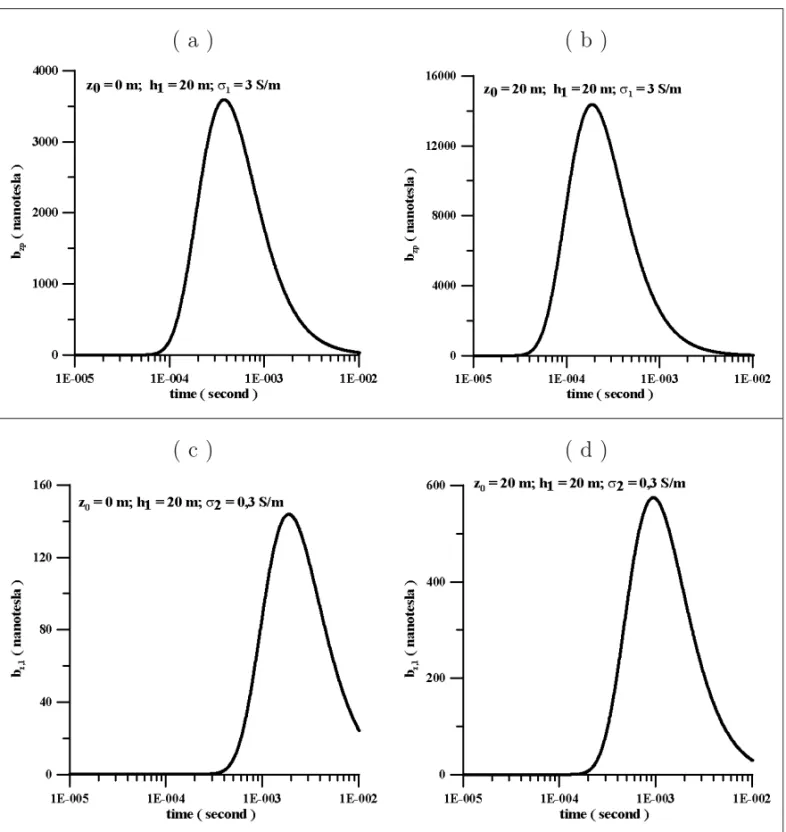
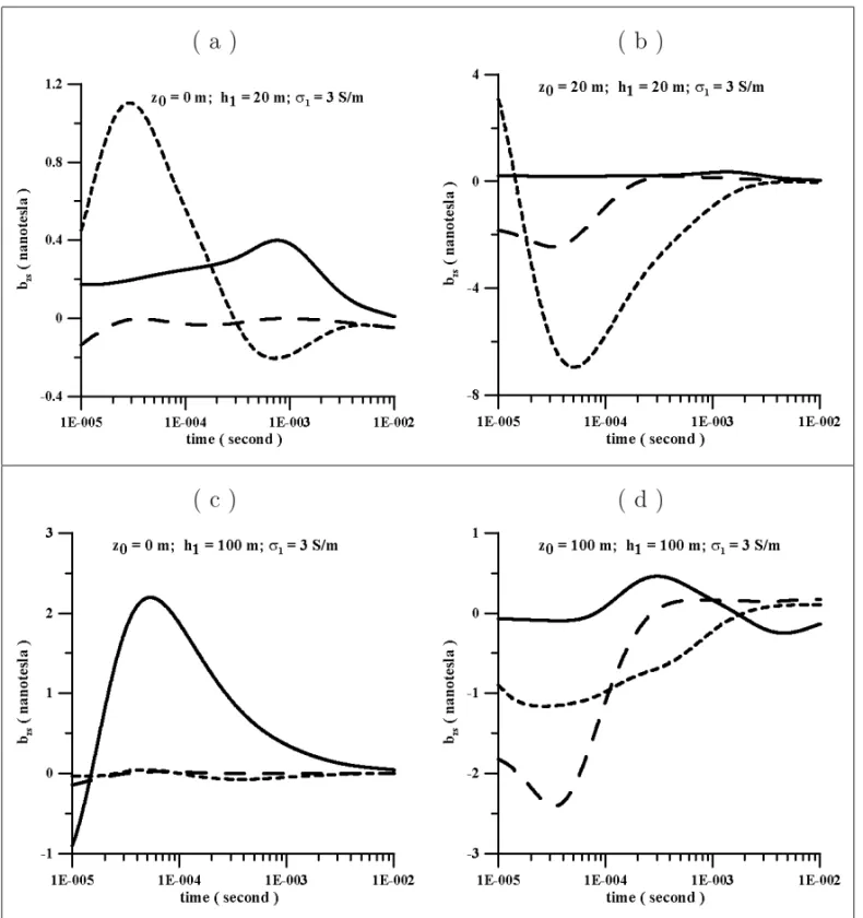
The graphs of Figure 3 represent the primary and the total field at the bottom of a 20 m water layer, overlying a substratum in which σ2 = 0.3 S/m. Both the magnitude and the time displacement of the
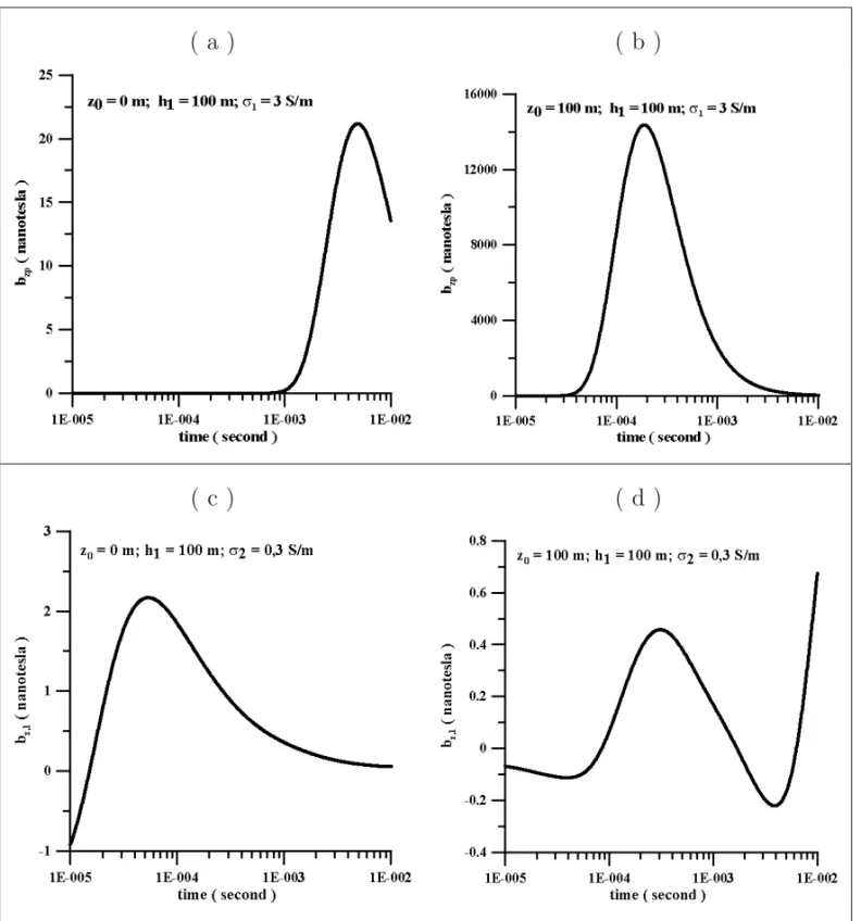
peaks of the curves are compatible with the source-receiver distances. The graphs of Figure 4 represent the primary and the total field at the bottom of an 100 m water layer, also overlying a substratum in which
σ2 = 0.3 S/m. In this case, the magnitude and the time displacement of the peaks of the curves are
compatible only for the primary field. The magnitude of the total field in Figure 4(c) is larger than in Figure 4(d), in spite of a smaller receiver-transmitter distance in this last one. The magnitude of the total field differs substantially between Figures 3(d) and 4(d), even though they have the same transmitter-receiver configuration. These two facts show the role that the thickness of the sea water layer plays in the secondary field.
If we neglect the length of the tail and assume the origin of the pulse at its center, we can estimate a group velocity,Vg, of the peak for the primary field under the conditions of Figures 3 and 4. The precision will be better for a larger transmitter-receiver distance. For instance: for Figure 4(a), Vg ≈25 km/s: and for Figure 3(a), Vg ≈70 km/s. In the present case, the phase velocity for the plane wave approximation under quasi-static conditions is given byVf =103√3.3 f. Since we may express the group velocity as:
Vg=
Vf 1−κd Vf
dω ,
( a )
( b )
( c )
( d )
Fig. 3 – Graphs of the time variation of the vertical component of the magnetic field for the case of a water layer with
h1=20 m and σ1=3 S/m, overlying a basement with σ2=0.3 S/m. Primary:bzp. Total:bz,1.
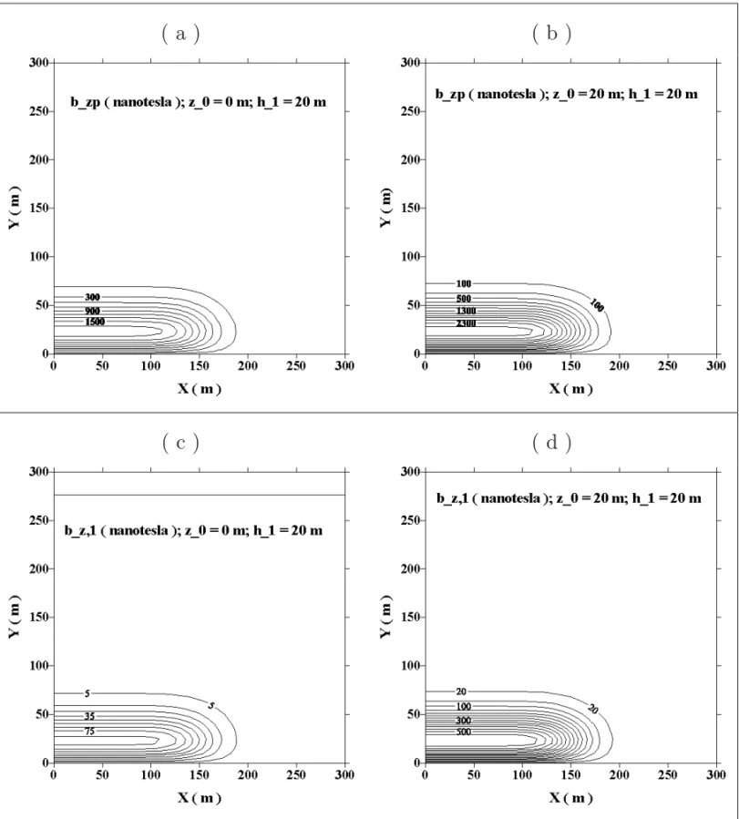
The contour maps of Figure 5 display the variation of the primary and the total field at the bottom of a 20 m water layer, overlying a substratum in which σ2 =0.3 S/m. All the maps show a perfect
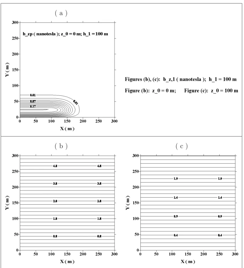
delin-eation of the tail position, and their magnitudes are also compatible with the transmitter-receiver distances. The contour maps of Figure 6 display the variation of the primary and the total field at the bottom of a 100 m water layer, also overlying a substratum in whichσ2=0.3 S/m. Only the primary field map shows
( a )
( b )
( c )
( d )
Fig. 4 – Graphs of the time variation of the vertical component of the magnetic field for the case of a water layer withh1=100 m andσ1=3 S/m, overlying a basement withσ2=0.3 S/m. Primary:bzp. Total: bz,1.
( a )
( b )
( c )
( d )
Fig. 5 – Contour maps of the vertical component of the magnetic field for the case of a water layer with h1=20 m and σ1=3 S/m and a substratum with σ2=0.3 S/m. Primary:bzp. Total:bz,1.
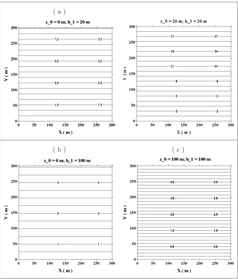
The graphs of Figure 7 show the contribution of the substratum to the secondary field for three values ofσ2: 0.3 S/m, 0.03 S/m, and 0.003 S/m. Together they show the influence that the conductivity of the
( a )
( b )
( c )
Fig. 6 – Contour maps of the vertical component of the magnetic field for the case of a water layer with h1=100 m and σ1=3 S/m and a substratum with σ2=0.3 S/m. Primary:bzp. Total:bz,1.
Figure 7(b) has a peak value five times larger than the peak value of Figure 7(a) for σ2 = 0.03 S/m
and even larger for σ2 = 0.003 S/m, but the magnitude ratio is inverse for σ2 = 0.3 S/m. A similar
behavior occurs between Figures 7(d) and 7(c). However, the curve forσ2 =0.03 S/m presents a value
smaller than the curve forσ2=0.003 S/m in graph (d), while the contrary occurs in graph (b). Therefore,
( a )
( b )
( c )
( d )
Fig. 7 – Graphs of the time variation of the main contribution of the substratum for the vertical component of the magnetic field:
σ2represents the conductivity of the substratum. (a) and (b)h1 = 20 m. (c) and (d)h1 =100 m. Solid line: σ2 = 0.3 S/m. Dotted line:σ2=0.03 S/m. Dashed line:σ2=0.003 S/m.
see maps of Figure 6(c) and (d). Under a 20 m water layer, the magnitudes are also of the same order of the total field of the maps of Figure 5 for transverse distances to the tail larger than 75 m. This means that, in shallow waters, it is necessary to separate the receivers at least one quarter of the tail lenght to achieve an adequate discrimination. Though this is not a problem in deep waters, one should consider the possibility of adverse situations as the referred case of Figure 9(d).
( a )
( b )
( c )
( a )
( b )
( c )
Fig. 9 – Contour maps of the difference of the vertical component of the magnetic field in nanotesla between one substratum withσ2=0.3 S/m and another withσ2=0.003 S/m.h1represents the thickness of the sea layer.
CONCLUSIONS
( a )
( b )
( c )
Fig. 10 – Contour maps of the difference of the vertical component of the magnetic field in nanotesla between one substratum withσ2=0.03 S/m and another withσ2=0.003 S/m.h1represents the thickness of the sea layer.
Though the source signal consists of a single pulse whose time duration is negligible, the conductivity of the sea water changes it appreciably. It increases its duration and causes the primary and the secondary fields to be measured up to times later than tens of milliseconds depending on the source-receiver offset. The curves of the graphs show this fact clearly, as well as the effect of the thickness of the sea layer on the relative magnitude of both the primary and the secondary fields. The contour maps show the influence of the thickness of the sea layer on the spatial variation of the field.
The model is adequate for shallow, intermediate, and deep water environments. For safety procedures, a step source model will be useful to evaluate transient fields at turn on and turn off times during field operations. The results provide a wealth of information depending on the selected source-receiver config-uration and the conductivity contrasts. The analysis, modelling, and interpretation of these data help to: define safety procedures in counter-sweep campaigns; map the conductivity of the submarine soil in envi-ronmental studies of marshes and bays; and identify, as a first approach, deep electrical structures, including possible economical deposits under the sea, employing mCSEMI (marine controlled source electromag-netic induction) methods in exploration and development works.
There are situations as show the maps of Figure 9, in which even for a high conductivity contrast the discrimination capability is poor. However, in general, the analysis of the magnitudes as a function of the electrical conductivity contrast, of the water layer thickness, of the transverse distance to the tail, and of the vertical position of the tail leads to evaluate the discrimination capability in the following way:
• it can be adequate for any conductivity contrast of the substratum as long as the measurement accuracy is better than about 0.01 nT;
• in shallow water it improves by increasing the receivers’ distance across the axis of the source and decreasing the distance between the tail and the seafloor; and
• for deep water it is in general adequate for any position of the receivers.
ACKNOWLEDGMENTS
This work has been supported with a grant and a fellowship from Conselho Nacional de Desenvolvimento Científico e Tecnológico (CNPq).
RESUMO
levantamento geofísico com uma fonte de corrente próxima ao assoalho do mar. Portanto, a presente análise pode servir: para definir parâmetros em contra-varredura de minas submarinas; para mapear a condutividade de sedimentos sob águas rasas em prevenção e controle de contaminação e como uma primeira abordagem na caracterização de depósitos minerais e de hidrocarbonetos no mar.
Palavras-chave:dipolos, energia eletromagnética, campos induzidos, mar.
REFERENCES
ABRAMOWITZM ANDSTEGUN IA. 1968. Laplace Transforms. In: ABRAMOWITZ MAND STEGUNIA (Eds),
Handbook of Mathematical Functions, Washington: National Bureau of Standards, p. 1020–1029.
AMUNDSENL, LØSETHL, MITTETR, ELLINGSRUDSANDURSINB. 2006. Decomposition of electromagetic
fields into upgoing and downgoing components. Geophysics 71: G211–G223.
BATISTALSANDSAMPAIOEES. 2003. Scattering of electromagnetic plane waves by a buried vertical dike. An
Acad Bras Cienc 75: 189–207.
CHAVEAD, CONSTABLE SC AND EDWARDSRN. 1991. Electrical Exploration Methods for the Seafloor. In:
NABIGHIANMN (Ed), Electromagnetic Methods in Applied Geophysics, vol. II, Application, Part B, Chapter
12, Tulsa SEG, p. 931–966.
CHAVEADANDCOXCS. 1982. Controlled electromagnetic sources for measuring electrical conductivity beneath
the the oceans, 1: forward problem and model study. Jour Geophys Res 87: 5327–5338.
CHEESMAN SJ, EDWARDSRN AND CHAVE AD. 1987. On the theory of seafloor conductivity mapping using
transient electromagnetic systems. Geophysics 52: 204–217.
CONSTABLE S. 2006. Marine electromagnetic methods – a new tool for offshore exploration. The Leading Edge
25: 438–445.
CONSTABLESANDCOXCS. 1996. Marine controlled-source electromagnetic sounding 2. The PEGASUS
exper-iment. Jour Geophys Res 101: 5519–5530.
CONSTABLESANDWEISSCJ. 2006. Mapping thin resistors and hydrocarbons with marine EM methods: insights from 1D modeling. Geophysics 71: G43–G51.
EDWARDSRN. 1997. On the resource evaluation of marine gas hydrate deposits using sea-floor transient electric
dipole-dipole methods. Geophysics 62: 63–74.
EIDESMO T, ELLINGSRUD S, MACGREGOR LM, CONSTABLE S, SINHA MC, JOHANSEN S, KONG FN AND
WESTERDAH H. 2002. Sea bed logging (SBL), a new method for remote and direct identification of
hydro-carbon filled layers in deepwater areas. First Break 20: 144–152.
ELLINGSRUDS, EIDESMOT, JOHANSENS, SINHAMC, MACGREGORLMANDCONSTABLES. 2002. Remote
sensing of hydrocarbon layers by seabed logging (SBL): results from a cruise offshore Angola. The Leading Edge 21: 972–982.
ERDÉLYIA (Ed). 1954. Tables of integral transforms, v. I, McGraw-Hill Book Co., New York.
FLOSADÓTTIRAHAND CONSTABLE S. 1996. Marine controlled-source electromagnetic sounding 1. Modelling
and experimental data. Jour Geophys Res 101: 5507–5517.
GUIMARÃESLGAND SAMPAIOEES. 2008a. Debye analysis applied to multiple reflections and attenuation of electromagnetic plane waves in a stratified sea substratum. J Quant Spectrosc Radiat Transf 109: 811–821.
GUIMARÃESLGANDSAMPAIOEES. 2008b. A note on Snell laws for electromagnetic plane waves in lossy media.
J Quant Spectrosc Radiat Transf 109: 2124–2140.
LØSETH LO AND URSIN B. 2007. Electromagnetic fields in planarly layered anisotropic media. Geophys Jour
Internat 170: 44–80.
PAPOULISA. 1962. The Fourier Integral and its Applications. San Francisco: McGraw-Hill Book Company, 318 p.
PINHEIROJCA ANDSAMPAIOEES. 1993. The magnetic field of the magnetic tail. In: PROCEEDINGS OF THE
CANNESCONFERENCE ONUNDERSEADEFENCETECHNOLOGY, p. 498–501.
RAYNER J. 2007. Geophysicists at war: mines, magnetism and memories Part 2: the Australian connection. Preview 30: 32–34.
SAMPAIOEESANDFOKKEMAJT. 1992. Scattering of monochromatic acoustic and electromagnetic plane waves
by two quarter spaces. Jour Geophys Res 97: 1953–1963.
SAMPAIOEESANDPOPOVMM. 1997. Zero-order time domain scattering of electromagnetic plane waves by two
quarter spaces. Radio Science 32: 305–315.
SCHOLLC AND EDWARDSRN. 2007. Marine downhole to seafloor dipole-dipole electromagnetic methods and
the resolution of resistive targets. Geophysics 72: WA39–WA49.
SOKOLOVI, KLAFTERJANDBLUMENA. 2002. Fractional kinetics. Physics Today 55: 48–54.
SOMMERFELDA. 1949. Partial Differential Equation in Physics, vol. VI. London: Academic Press, 335 p.
SOUZA H AND SAMPAIO EES. 2001. Apparent resistivity and spectral induced polarization in the submarine environment. An Acad Bras Cienc 73: 429–444.
SPIESBRANDHABASHYTM. 1995. Sensitivity analysis of crosswell electromagnetics. Geophysics 60: 834–845.
STRATTONJA. 1941. Electromagnetic Theory. New York: McGraw-Hill Book Company, 615 p.
TORRES-VERDÍN C AND BOSTICK JR FX. 1992. Implications of the Born approximation for the magnetotel-luric problem in three-dimensional environment. Geophysics 57: 587–602.
TORRES-VERDÍNC AND HABASHY TM. 2001. Rapid numerical simulation of axisymmetric single-well induc-tion data using the extended Born approximainduc-tion. Radio Science 35: 1287–1306.
TSENGHW, LEEKH ANDBECKERA. 2003. 3-D interpretation of electromagnetic data using a modified exten-sion Born approsimation. Geophysics 68: 127–137.
WAITJR. 1982. Geo-electromagnetism. New York: Academic Press Inc, 268 p.
WANNAMAKER PE, HOHMANN GW AND SANFILIPO WA. 1984. Electromagnetic modeling of
three-dimen-sional bodies in layered earths using integral equations. Geophysics 49: 60–74.
WARDSHANDHOHMANNGW. 1988. Electromagnetic theory for geophysical application. In: NABIGHIANMN
(Ed), Electromagnetic Methods in Applied Geophysics, vol. I, Theory, Chapter 3, Tulsa, SEG p. 130–311.
WOLFGRAMPA, EDWARDSRN, LAWLKAND BONEMN. 1986. Polymetallic sulfide exploration on the deep
sea floor: The feasibility of the MINI-MOSES experiment. Geophysics 51: 1808–1818.
WYNN JS. 1988. Titanium geophysics – the application of induced polarization to sea-floor mineral exploration.
APPENDIXES
A BINOMIAL EXPANSION OF THE KERNEL FUNCTIONS
Take into account that|e−2α1h1|<1 and|R1
,j|<1, j =0,2, and express the reflection coefficient as,
R1,j = 2α1 α1+αj −
1, j =0,2.
Next, expand the denominator ofFx±,1(λ,s) by the binomial theorem and neglect second and higher order
terms to obtain:
Z β+i∞
β−i∞
Fx+,1(λ,s)
s e
+α1ze+s tds
≈
Z β+i∞
β−i∞
2
λ s(α1+α2) −
λ sα1
e−α1q1
+
−s(α12λ
+α0) −
2λ s(α1+α2)+
λ sα1
e−α1q2
e+stds,
Z β+i∞
β−i∞
Fx−,1(λ,s)
s e
−α1ze+s tds
≈
Z β+i∞
β−i∞
2
λ s(α1+α0) −
λ sα1
e−α1q3
+
− 2λ
s(α1+α0) −
2λ s(α1+α2)+
λ sα1
e−α1q4
e+stds. (A1)
Equations A1 contain three types of Laplace transforms. The coefficientsqj are positive, j =1,2,3,4, because
q1=2h1−z−z0; q2=2h1−z+z0; q3=z+z0; q4=2h1+z−z0.
Whenz =h1,
q1=h1−z0; q2=h1+z0; q3=h1+z0; q4=3h1−z0.
B LAPLACE TRANSFORM OF THE FIRST ORDER TERMS
Substitute in Equation A1 s = p−γ, γ = μλ2
0σ1 and write:
α0=
√
(p−p0)(p− ˙p0)
c0 ; α1=
√
μ0σ1√p; and α2=√μ0σ2√p+p1,
where p=0, p0=γ +i c0λ, p0˙ =γ −i c0λ, and
p1= λ 2(σ1
−σ2)
μ0σ1σ2 =
γ (σ1−σ2) σ2
represent the four branch points. The residue at the pole p = +γ vanishes. The vertical straight line in
Figure B1 represents the Bromwich path. We shall evaluate the integrals modifying it to a closed circuit (Papoulis 1962).
• −p1
• γ
Plane (p)
ℜ(p)
ℑ(p)
• p0
•
˙
p0
•
β+γ+iΩ
β+γ−iΩ
β+γ
Fig. B1 – Distortion of the Bromwich path (ℜ(p)=β+γ) into a closed contour for the integration of Equations B1, B2, and B4. The function is analytical inside the contour. The origin,−p1, p0, andp˙0 are branch points, andγ is the pole.
FIRSTTRANSFORM
λ Z
Br
e−α1qjest
sα1 ds =
e−γt 2
Z
Br
1
√p(
−√γ +√p) −
1
√p(
+√γ +√p)
e−√μ0σ1qj√pe+ptd p,
4 X
j=1
(−1)jλ
2πi Z
Br
e−α1qjest
sα1 ds =
4 X
j=1 (−1)j
e−λqj
2 er f c
−λχ+ qj
2χ
−e
+λqj 2 er f c
+λχ+ qj
2χ
u(t), (B1)
where:
χ = r
t μ0σ1.
The circuit of the two integrals of Equation B1 is represented in Figure B1 with the following parts: the semi-circle→ ∞, forℜ(p) < β +γ; the circleǫ →0 around the branch point p =0; the contour
of the branch cut (−∞ → 0); and the circle around the pole p = +γ. The two terms of Equation B1
correspond to the contour of the branch cut. The integrals along the circleǫ →0 around the branch point p=0 and along the semi-circle→ ∞ forℜ(p) < β+γ vanish.
SECONDTRANSFORM
Z
Br
e−α1qjest
s(α1+α2)ds = e
−γt
Z
Br
√σ1√p
−√σ2√p+ p1e−√μ0σ1qj√pe+pt
√μ0(σ1
4,j6=3 X
j=1
(−1)j+1λ πi
Z
Br
e−α1qjest
s(α1+α2)ds = 4,j6=3
X
j=1
(−1)j+1g+j(λ,t)u(t). (B2)
The circuit of the two integrals of Equation B2 is represented in Figure B1, and is constituted of the following parts: the semi-circle→ ∞, forℜ(p) < β+γ; the circlesǫ →0 around the branch points
p = 0 and p = −p1; the contours of the branch cuts: (−∞ → 0) and from−p1 to 0; and the circle
around p = +γ. In Equation B2, the integrals along the circles with radius ǫ → 0 around the branch
points p=0 and p= −p1 and around p=→ ∞ vanish, and
∂g+j(λ,t)
∂t =
2λe−γt√σ1
√μ0(σ1
−σ2)
1
√
πte
−
q2 j
4χ2 + λχe
+λ2χ2
2√t
×
e−λqj er f c
−λχ+ qj
2χ
−e+λqj er f c
λχ+ qj
2χ
+
√σ2(σ1
−σ2)√p1
π√σ1
Z 1
0
N+(p) (σ1−σ2)p+σ2e
−p1t pd p
, (B3)
N+(p)=p1− p sin √μ0σ1p1qj√p
.
THIRDTRANSFORM
Z
Br
e−α1qjest
s(α1+α0)ds = e−γt μ0ǫ0
Z
Br
√μ0σ1√p e−√μ0σ1qj√pe+pt
(p−γ )2(γ +σ1
ǫ0 −p)
d p
−e
−γt
μ0ǫ0 Z
Br
√
(p− p0)(p− ˙p0)e−√μ0σ1qj√pe+pt
c0(p−γ )2(γ +σ1
ǫ0 −p)
d p,
4 X
j=2
(−1)j+1λ πi
Z
Br
e−α1qjest
s(α1+α0)ds = 4 X
j=2
(−1)j+1ng−j(λ,t)+h−j(λ,t)ou(t). (B4)
The circuit of the two integrals of Equation B4 is represented in Figure B1, and is constituted of the following parts: the semi-circle → ∞, forℜ(p) < β +γ; the circlesǫ → 0 around the branch
points p = 0, p = p0 and p = ˙p0 and of the pole p = +γ; and the contours of the two branch cuts:
from p0˙ to p0 and from−∞ to 0. The pole p =γ + σ1
ǫ0 is not shown, and its two residues cancel out.
In Equation B4 the integrals along the circles with radiusǫ →0 around the branch points p=0, p= p0
and p = ˙p0, as well as around p = → ∞, vanish. The term g−j(λ,t) on the right-hand side of
contour around the branch cut parallel to the imaginary axis, such that
∂g−j(λ,t)
∂t =
2λe−γt
√μ0σ1
λχe+λ2χ2
2√t
e−λqj er f c
−λχ+2qj
χ
−e+λqj er f c
λχ+2qj
χ
−
q γ +σ1
ǫ0 e +γt+σǫ10t
2
e−
q γ+σǫ10
√μ 0σ1qj
er f c
−
r
(γ +σ1
ǫ0)t+ qj 2χ
−e+
q γ+σǫ01
√
μ0σ1qj
er f c
+
r
(γ +σ1 ǫ0)t+
qj 2χ
+2c0λe
−γt
π
Z +∞
0
N−e−t p
(p+γ ) (p+γ +σ1
ǫ0)
d p,
N−(p)=p(p+ p0)(p+ ˙p0)sin(√μ0σ1qj√p). (B5)
∂h−j(λ,t)
∂t = −
4c0λ π
Z c0λ
0
σ1 ǫ0
sin(pt−bj)
p +cos(pt−bj)
q
c02λ2− p2e−aj
σ12 ǫ02 +p
2 d p, (B6)
aj =
r μ0σ1
2
q p
γ2+p2+γ qj,
bj =
r μ0σ1
2
q p
γ2+p2−γ qj.
C FIRST HANKEL TRANSFORM
The first two terms on the right-hand side of Equation 15 yield the following Hankel transforms:
(T H)1 = −
∂ ∂y
Z +∞
0
λe−λ2χ2 J0(λr)
dλ, = +y
r
Z +∞
0
λ2e−λ2χ2 J1(λr)dλ. (C1)
Employing the tables of (Erdélyi 1954) we obtain the following result:
(T H)1 = −
1
2χ2
Ŵ(1) ∂
∂y 1F1 1;1; − r 2χ 2!! , = + y
4χ4
(0!) e−
r
2χ 2
L10
r
2χ 2!
. (C2)
Employing the properties of theŴ(η) function, of Kummer’s hypergeometric series, and of the generalized
Laguerre polinomium on Equation C2, we conclude that
(T H)1 =
y
and therefore:
100y Z +L2
−L2
Z +∞
0
4
X
j=1
(−1)je−(q j2χ)2 λ 2e−λ2χ2
√
π μ0σ1χ
J1(λr)dλ
d x0 r
= π σ1y e
(−2yχ)2
105t2
er f x
+ L2
2χ
−er f x
− L2
2χ
4 X
j=1
(−1)je−(2q jχ)2
, (C4)
100y Z +L2
−L2
Z +∞
0
4, j6=3 X
j=1
(−1)j+1e−(q j2χ)2 2λ 2e−λ2χ2
√
π μ0(σ1−σ2) χ
J1(λr)dλ
d x0 r
= 2π σ
2 1 y e(−
y
2χ)2
105(σ1
−σ2)t2
er f x
+ L2
2χ
−er f x
− L2
2χ
4, j6=3 X
j=1
(−1)j+1e−(q j2χ)2
. (C5)
D SECOND HANKEL TRANSFORM
The two first terms inside the brackets on the right-hand side of Equation 16, combined with Equation 13, yield the following Hankel transform:
(T H)2 = +
4 − σ2
σ1 ∂ ∂y
Z +∞
0
λ2e−λ2χ2 J0(λr)dλ,
= −
4 − σ2
σ1 y r Z +∞ 0
λ3e−λ2χ2 J1(λr)dλ. (D1)
By employing the tables of (Erdélyi 1954) we obtain the following result:
(T H)2 = +
4 − σ2
σ1
1 2χ3
Ŵ 3 2 ∂ ∂y 1F1
3 2;1; −
r 2χ 2!! , = −
4 − σ2
σ1 y
4χ5
1 2! e− r 2χ 2
L11 2 r 2χ 2! . (D2)
We shall prove that the two forms in Equation D2 give the same result. First consider the following properties ofŴ(η): Ŵ 12=√π; Ŵ(η+1)=η Ŵ(η)=η!; and
Ŵ
n+1
2
= 5
n−1
k=0(2n+1)
2n Ŵ
1
2
.
Employing the general expression of Kummer’s confluent hypergeometric series,
1F1 a;b; − r 2χ 2! = ∞ X
n=0
(−1)nŴ(a+n)/ Ŵ(a) (Ŵ(b+n)/ Ŵ(b))n!
r2
4χ2 n
,
1F1 3
2;1; −
r 2χ 2! = ∞ X
n=0
(−1)n 5n
k=0(2k+1)
2n(n!)2
r2
4χ2 n
we obtain:
∂ ∂y 1F1
3 2;1; −
r 2χ 2! = 2y r2 ∞ X
n=1
n(−1)n 5nk=0(2k+1)
2n(n!)2
r2
4χ2 n
.
Also taking into account the representation of Laguerre’s generalized polynomial of order η and
coef-ficient α
Lαη(χ )=
eχχ−α
η!
dη dχη e
−χχη+α
,
we obtain
L11 2(χ )=
eχχ−1 1 2!
!
d12
dχ12
e−χχ32
!
.
According to (Sokolov et al. 2002)
d12χμ
dχ12 =
Ŵ(μ+1) Ŵ(μ+12)χ
μ−12, μ >−1.
Applying fractional derivative to the Taylor’s series expansion of the exponential function, we conclude that
d12
dχ12
e−χχ32
!
=
∞
X
p=0 (−1)p
(p)!
Ŵ(p+52) Ŵ(p+2)χ
p+1,
where: Ŵ(p+2) = (p+1)! and
Ŵ
p+ 5
2
= Ŵ
(p+2)+1
2
= 5
p
k=0(2k+3)
2p+2 Ŵ 1
2
.
Therefore, we may rewrite Equation D2 as:
(T H)2 =
4−σ2
σ1
√
πy
2χ3r2
∞
X
n=1
n(−1)n 5nk=0(2k+1)
2n(n!)2
r
2χ 2n
. (D3)
Substituting Equations D3 and C3 in Equation 13, we obtain the following expression for bzs in nanotesla:
bzs(R,t) =
25y
√
π μ0σ1χ3
2π
4−σ2
σ1
∞
X
n=1
n(−1)n 5nk=1(2k+1) y2n−1
23n(n!)2χ2n
n
X
j=1
(n−1)!
(2j−1) (j−1)!(n− j)!
x
+ L2 y
2j−1
−
x
− L2 y
2j−1
+ √
πe−
y
2χ 2
e−
z−z
0 2χ
2
+e−
z+z
0 2χ 2 χ er f x
+ L2
2χ
− er f
x
− L2
2χ
. (D4)
The calculus of the double series of Equation D4 becomes laborious for high values of the argument. So, it is necessary to analyze its asymptotic behavior when y andt are such that χy >> 1. The fact that
lim
η→−∞1F1
3
2;1;η
= Ŵ(1)
Ŵ −12 (−η)
implies that
lim
r
2χ 2
→∞
1F1 3
2;1; −
r
2χ 2!
= − 4χ
3
√
πr3,
lim
r
2χ 2
→∞
∂ ∂y 1F1
3 2;1; −
r
2χ
2!!
= 12yχ
3
√
πr5
and consequently we have:
12yχ3
√
π
Z +L2
−L2
d x0 r5 =
4χ3
√
πy3
(x+L/2)(3y2+2(x+L/2)2) (y2+(x +L/2)2)3/2 −
(x−L/2)(3y2+2(x−L/2)2) (y2+(x −L/2)2)3/2