The DC field components of horizontal and vertical electric dipole sources immersed in three-layered stratified media

The DC field components of horizontal and vertical electric dipole

sources immersed in three-layered stratified media

D. Llanwyn Jones, C. P. Burke

Physics Department, King’s College, Strand, London, WC2R 2LS Received: 24 September 1996 / Accepted: 3 December 1996

Abstract. Formulas for computing the Cartesian com-ponents of the static (DC) fields of horizontal electric dipoles ( HEDs) and vertical electric dipoles ( VEDs) located in the central zone of a three-layer horizontally stratified medium are derived and presented in a summary form suitable for immediate computation. Formulas are given for the electric and magnetic field components in the upper and central regions. In the general case the computation involves the summation of a convergent infinite series. For the particular case of an infinitely thick central region (corresponding to the two-layer problem), the analysis produces relatively simple closed-form equations for the field components which are suitable for a ‘hand calculation’. Specimen calcula-tions for dipoles in seawaters are included and the derived results are compared with computations made using an ac model.

1 Introduction

The subject of the electromagnetic fields excited by buried or submerged radiation sources is of interest both for remote sensing and for communication purposes. Current elements or probes with various configurations may be utilised as sources. Additionally, it is known that earthquakes generate a characteristic precursor at ultra-low (and higher) frequencies (e.g. Molchanov et al., 1992; Parrot et al., 1995) and the formulas presented here may be of value in estimating the source magnitude from measurement of ULF fields on the Earth’s surface. A seminal paper dealing with the ac fields of a submerged source for the three-layer case is that of Weaver (1967). An excellent compendium of simplified formulas for the two-layer case is given in Kraichman’s book (1976) and further formulas for this model have

been published in a series of papers by Bannister (see e.g. Bannister, 1984). Developments in relation to the ocean/lithosphere environment have been presented, for example, by Chave and Cox (1982) and Fraser-Smith

et al.(1988). Often in geophysics, point current sources and sinks are used to produce subsurface fields for remote sensing, and the configuration used is such that the source acts essentially as a dipole (Wait 1982, 1993). An important feature of the ac formulation is the presence of ‘lateral waves’ which aid the propagation of the fields. These waves are not present in the dc case. A large number of relevant mathematical and practical results for ac and dc are presented by Wait (1982), but the dc formulas in this paper (for the three-layer case) have not been published previously. Here we concen-trate upon these dc (or static) solutions which apply for vanishing small values of r=k.

The mathematical background to our formulation is that developed by Sommerfeld (1967) and, particularly, Wait (1987). In Burke and Jones (1992, 1993, 1994), we considered an ac radiation source located in seawater – the central region of a three-layered horizontally strati-fied medium. We assumed a time-harmonic source dipole moment of angular frequency x, and presented integral formulas of the Sommerfeld type for the two-component Hertz vector …Px;0;Pz† which is required for the solution in the case of horizontal electric dipole (HED) radiation source and the single-component Hertz vector …0;0;Pz† needed for the vertical electric dipole (VED). We also gave explicit formulas from which the Cartesian components of the E and B fields can be computed by quadrature. The field expressions are the sum of two parts – an analytic primary contribution which is the field produced in a medium of infinite extent, and an integral secondary contribution arising from the presence of the interfaces. These previous formulas are valid at any wave frequency, including, particularly, the dc case,xˆ0.

For the dc case, we show that the integral formulas can be evaluated analytically using Laplace transforms. This process leads to an infinite series expansion suitable Correspondence to:D. Llanwyn Jones

(email) [email protected]

for computation. Each term of the infinite series corresponds to a particular image of the source in the upper or the lower interface. Needless to say, the application of the infinite series produces a much faster algorithm for computing the field components at dc than any involving numerical integration.

It is customary to determine dc solutions by deriving formulas for a scalar electric potential and a vector magnetic potential. In this paper, however, we derive dc analytic formulas from our pre-existing ac equations derived from a Hertz vector. In part, this work was undertaken to validate our ac field derivations and computer code (Burke and Jones, 1992, 1993). The results for the various dc field components are given in a compact tabular form for reference and computational purposes. We also give specimen numerical data.

2 The physical model

We first consider an HED of current moment Id`( Am) placed in the central (conducting) layer of a three-layer, horizontally stratified medium. The upper region is taken to be free space and the lower two regions are conductors with conductivitiesr2 andr3 (S/m),

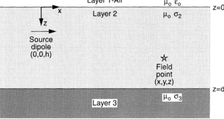
respec-tively. The three regions could represent a geophysical air-overburden-basement or an oceanic air-sea- seabed problem. Cartesian co-ordinates are used withzdirected downwards, zˆ0 being the upper interface. The magnetic permeability is assumed to be that of free space everywhere, so the dc fields of a magnetic dipole source are unaffected by the interfaces and are the same as those of a magnetic dipole located in free space. The three layers are of infinite extent in the x and y directions. The geometry is illustrated in Fig. 1.

The HED source isx-directed and located at…0;0;h†. The central region is of thicknessd; the upper and lower regions are assumed to be of infinite thickness. Fields are to be computed at the point…x;y;z† with ÿ1 zd, i.e. anywhere in layers 1 or 2. If it is assumed that r2 ˆr3 (or, alternatively, thatd ! 1), only the upper

interface affects the solution. This is termed the ‘two-layer’ or ‘thick-‘two-layer’ solution in distinction to the ‘thin-layer’ solution obtained for finite d for which both interfaces (upper and lower) materially affect the field components.

3 The field equations for the HED

3.1 Derivation of the HED dc field equations

In Burke and Jones, 1992, §3 (henceforth Ref. 1), general equations were presented for the two components of the Hertz vector in layer i, Pxi and Pzi, produced by an HED source dipole located in layer iˆ2. Using the notation of this previous paper, we now consider the limit x!0 to deduce the appropriate formulas for the dc case. When the formulas for the components of the Hertz vector have been established, the static _E and H field vectors can be computed in any layer from the standard expression (e.g. Stratton, 1941),

E ˆk2P‡grad div_P; …1†

Hˆr3curl_P; …2†

where k2ˆ ÿixl₀r3 andr3ˆ …r‡ix† is the complex conductivity of the layer in which the field is to be computed. At dc, in layer 2, r3ˆr2 and is real, but in

layer 1, r3ˆix0, and some care has to be taken in evaluating the limit of the right-hand side of Eq. (1) as x!0.

3.1.1 HED fields in layer 2

At dc, the Sommerfeld parameter uˆ …k2ÿk2†12 _which

appears in the ac formulation (Ref. 1) may be replaced byk. Thus, for the dc case, the components of the Hertz vector in layer 2 are written in the form,

Px2ˆM Z ₁

0

eÿkjzÿhj‡Beÿkz‡Cekz

J0…kq†dk; …3†

Pz2ˆM @ @x

Z 1

0

Teÿkz‡Sekz

ÿ 1

J0…kq†dk; …4†

where MˆId`=…4pr2†;q2_ˆx2_‡y2 _{and J}

0 is the Bessel

function of the first kind of order zero.

Explicit expressions for the four coefficientsB, C, S

andTwere given in Ref. 1. These expressions involved, h and z, together with the layer conductivities which enter the equations in terms of the interfacial reflection coefficients for horizontal…Rij†and vertical polarisation

…Rjjij† for fields incident from layer i onto the interface with layer j. It is immediately seen from the results of Ref. 1 that asx!0,

R21ˆR23ˆ0; …5a†

and

Rjj₂₁ˆ ÿ1; Rjj₂₃ˆ …r3ÿr2†=…r3‡r2†: …5b†

It follows from the first two of these that the coefficients

BandCin the expression forPx2 are both zero, so that

Px2is unaffected by the presence of the interfaces. It then

follows from Sommerfeld’s ac formula [Sommerfeld, 1967, p242, Eq. (14)] that, at dc, Px2 is expressible in

closed form:

Px2 ˆM Z 1

0

eÿkjzÿhjJ0…kq†dkˆM q2‡ …hÿz†2

h iÿ1

2

: …6†

It is noted that this integral can be also be represented as a known Laplace transform; see, for example, Abramo-witz and Stegun (1968, Transform #29:3:55; p. 1024), which gives a direct way of obtaining the result of Eq. (6) for the dc case. Equation (6) gives the primary field of the dipole, i.e. the field of a dipole located in a medium of infinite extent.

When the differential in Eq. (4) is evaluated, the expression forPz2 becomes

Pz2ˆ ÿM

x q

Z ₁

0

kÿSekz‡Teÿkz1J1…kq†dk; …7†

J1 being the Bessel function of the first kind of order

one. At dc, the coefficientsSand Tare (Ref. 1)

Sˆ ÿ…Rjj23=Djjk† eÿk…2d‡h†‡eÿk…2dÿh†

…8a†

and

T ˆ ÿ…1=Djjk† eÿkhÿRjj₂₃eÿk…2dÿh†

; …8b†

where Djjˆ1‡Rjj₂₃eÿ2kd_.

We now expand the factor 1=Djj as a geometric progression

1=DjˆX

1

nˆ0 ÿRjj₂₃

n

eÿ2ndk: …9†

It then follows thatPz2 can be expressed as the sum of

four terms:

Pz2ˆ X4

iˆ1

P_z…i₂†ˆP_z…1₂†‡P_z…22†‡P…_z3₂†‡P…_z4₂†; …10a†

with

P…_z1₂†ˆ ‡M x q

Z ₁

0

eÿk…h‡z†X

1

nˆ0 ÿRjj₂₃

n

eÿ2ndkJ1…kq†dk;

…10b†

P…2†_z2 ˆ ÿM

x q

Z 1

0

Rjj23eÿ

k…2dÿh‡z†X1

nˆ0 ÿRjj23

n

eÿ2ndkJ1…kq†dk;

…10c†

P…3†_z2 ˆ ‡M x q

Z ₁

0

Rjj23eÿ

k…2d‡hÿz†X 1

nˆ0 ÿRjj23

n

eÿ2ndkJ1…kq†dk;

…10d†

P…_z4₂†ˆ ‡M x q

Z ₁

0

Rjj₂₃eÿk…2dÿhÿz†X

1

nˆ0 ÿRjj₂₃

n

eÿ2ndkJ1…kq†dk:

…10e†

Consider the termP…_z1₂†. This may be written as

P…_z1₂†ˆM x q

Z 1

0 X1

n_ˆ0 ÿRjj₂₃

n

exp…ÿkrn1†J1…kq†dk; …11†

where rn1ˆ2nd‡h‡z.

As was the case for Eq. (6), the integral in Eq. (11) can be evaluated using a tabulated result for the Laplace transform (Abramowitz and Stegun, 1968, Transform #29.3.56, p. 1024) viz:

Z ₁

0

aeÿstJ1…at†dtˆps2_‡a2_ÿsp_s2_‡a2ÿ1_:

For small values of a=s, greater numerical accuracy is obtained by recasting the right-hand side of this formula using the identity:



s2_‡a2 p

ÿs



s2_‡a2 p

ÿ1

a2s2‡a2‡sps2‡_a2ÿ1:

Puttingaˆq; tˆkandsˆrn1, it follows that

P…_z1₂†ˆ ‡M xX

1

nˆ0 ÿRjj₂₃

n

rn21‡q 2_‡

rn1



r2_n1‡q2 q

:

…12a† It is noted that for a thick central layer, with h and z finite so that dh‡q‡z, only thenˆ0 term of this series expansion survives. This term is that produced by the image of the source dipole in the upper interface and is a secondary field component. Further secondary components are produced by the higher values ofn.

Applying the same technique to the remaining terms in Eq. (10), we obtain

P…_z2₂†ˆ ‡M xX

1

nˆ1 ÿRjj₂₃

n

rn22‡q 2_‡

rn2



r2_n2‡q2 q

;

…12b†

P…_z3₂†ˆ ÿM xX

1

nˆ1 ÿRjj₂₃

n

r_n2₃‡q2‡rn3



r2

n3‡q2 q

;

…12c†

P…z42†ˆ ÿM x X1

nˆ1 ÿRjj₂₃

n

rn24‡q 2_‡

rn4



r2n4‡q2 q

;

…12d† with rn2ˆ2ndÿh‡z; rn3ˆ2nd‡hÿzand rn4 ˆ2nd ÿhÿz.

Note that in Eq.(12b–d) the summations do not include the termnˆ0. These three terms thus make no contribution to the solution when d is very large, provided that hand zare finite.

The solution presented is, in fact, a geometrical-optics (or images) formula which, as is well known, is valid when the reflection coefficient is independent of the ‘angle of incidence’. In the given formulation this angle of incidence is embodied within the Sommerfeld ‘dum-my’ variable k. The images associated with a positive sign precedingzin the formulas forrniare in layer 1 and those with a negative sign are in layer 3.

3.1.2 HED dc fields in layer 1

Again, referring to the ac formulas presented in Ref. 1, it is easily seen that, at dc, the Hertz vector components Px1andPz1in the air-space (layer 1) may be represented

in the form

Px1 ˆM Z ₁

0

A ekzJ0…kq†dk; …13†

Pz1ˆM @ @x

Z 1

0

R ekzJ0…kq†dk; …14a†

ˆ ÿM x q

Z ₁

0

kR ekzJ1…kq†dk: …14b†

Application of the boundary conditions across the interfaces zˆ0 and zˆd (as described in Ref. 1) produces the following results for the two coefficientsA and Rasx!0:

Aˆ ÿ… ir2=xe0†eÿkh; …15a†

Rˆ ÿ… ir2=xe0†…S‡T† ˆ …1=k†…ir2=xe0†eÿkh: …15b†

Hence, as x!0, both A and R, and thus Px1 and

Pz1! 1. However, Eqs. (1) and (2) must give finite

values for the dc fieldsEandH. In Eq. (1)k2P!0 and in Eq. (2)ixe0r 2_Pis clearly finite. We will now show that in Eq. (1), rr 1_Pis also finite.

3.1.2.1 Calculation of r 1Pand henceE. From Eqs. (13) and (14) and the elementary formula

r 1Pˆ @Px=@x‡ @Pz=@z it is found that

r 1Pˆ ÿM x q

Z 1

0

k…A‡kR†ekzJ1…kq†dk: …16†

In Eq. (16) the factorA‡kRis indeterminate asx!0 if Eq. (15) is used. To resolve this indeterminacy we return to the boundary condition that both Ex and Ey and hencer 1_Pis continuous across the interfacezˆ0. At dc this requires that

A‡kRˆeÿkh‡k…SÿT†

ˆ 2=Djj

eÿkhÿRjj₂₃eÿk…2dÿh†

; …17†

and thus

r 1Pˆ ÿ2M x q

Z 1

0

k=Djj

eÿkhÿRjj₂₃eÿk…2dÿh†

2ekzJ1…kq†dk:

In this formula the integrand may be cast into the same form as that previously expanded [Eq. (10)] by noting that it is equivalent to

r 1Pˆÿ2Mx q

@ @z

Z 1

0

1=Djj

eÿk…hÿz†ÿR₂₃jj eÿk…2dÿhÿz†

2J1…kq†dk: …18† Proceeding as in Sect. 3.1.1, we then find the following series expansion formula for Eq.(18).

r 1Pˆ ÿ2Mx @ @z

X1

nˆ0

ÿRjj₂₃ n

r_n2₃‡q2‡rn3

 r2

n3‡q2

q

"

‡X1

nˆ1

ÿRjj₂₃ n

r2_n4‡q2‡rn4

 r2

n4‡q2

q

#

: …19†

By evaluating the gradient of Eq. (19) in accordance with Eq. (1), we obtain the series expansion formulas for the electric field components in layer 1. These are given in Sect.4.2. Note that the nˆ0 term in Eq. (19) represents the sum of the primary (or direct) field plus the ‘thick-layer’ field corresponding to d ! 1, these being equal for a point in layer 1. Also only the images in layer 3 contribute to the field in layer 1 [rn1andrn2are

absent in Eq. (19)].

3.1.2.2 Calculation of H (or B). _H is given by Eq. (2) with r3 ˆixe0 for layer 1. From Eq.

(15),ixe0Aˆr2eÿkh andixe0Rˆ ÿr2…1=k†eÿkh. It then

follows that [as for Eq. (6)],

ixe0Px1 ˆMr2 Z 1

0

eÿk…hÿz†J0…kq†dk

ˆMr2 q2‡ …hÿz†2

h iÿ1

2

;

…20†

and

ixe0Pz1ˆMr2

x q

Z 1

0

eÿk…hÿz†J1…kq†dkˆMr2x

2 q2‡…hÿz†2‡…hÿz†q2‡…hÿz†2

h i1

2

ÿ1

:

…21† The magnetic field components in layer 1 may now be computed asHˆ r 2 …ixe0P†, thexandzcomponents

of the vector P being given by the closed form expressions, (20) and (21). Interestingly, these dc magnetic field components are independent of d; r2

and r3 (note that Mr2ˆId`=4p). The field formulas

derived from Eqs. (20) and (21) are given in Sect. 4.2.

4 Recipes for computing the HED dc field components

4.1 HED DC Fields in Layer 2

The field equations for computing E and Bˆl0H, derived from the formulas of Sect. 3 are given in Tables 1 and 2. The field components are computed using the tables as follows.

a) First compute the primary (direct) field produced by the source dipole using the equations in Table 1, [derived from Eq. (6)]. These are the fields produced by the source if located in a medium of conductivity r2

which is of infinite thickness. These results are well known and can be put in the form presented in the table using formulas presented in many standard texts (e.g. Stratton, 1941, p. 436).

(the ‘thick-layer’ case). This is done by using the formulas of Table 2 with iˆ1 and nˆ0. These for-mulas are obtained from the nˆ0 term of Eq. (12a). The only value ofrni required is thus

r01ˆh‡z:

Add these field values to those obtained in stage (a). The result is that for the fields produced by a source at finite depth within an infinitely thick central layer, and the fields are thus affected by the upper interface only. The source of this term is the image dipole located in layer 1 at a distancehabove the upper interface.

c) To find the field for the general thin-layer or three-layer case the results of Table 2 are used in the following manner. If F represents any one of the field formulas given in the second column of Table 2 compute the double summation:

X1

nˆ1 X4

iˆ1

Fni

" # :

Repeat this calculation for the five finite components in Table 2. The convergence of the summation depends on the value ofR (which is the reflection coefficient of the

lower interface, Rjj₂₃) and on the spatial parameters, particularly the layer thicknessd (Rsmall and/ordlarge gives rapid convergence). The double summation com-putes the fields given by the n>0 terms of Eq. (12) which are the fields of the multiple images of the source in the upper…iˆ1;2†and lower …iˆ3;4†layers.

The final result is obtained by adding the field produced in step (c) to that produced at step (b). If the i-summation is first computed for nˆ1 and the result added to that of step (b), the convergence can be tested following each successive n-summation enabling a sim-ple algorithm to be devised for terminating the summa-tion with a machine of any given precision.

d) Note: if the middle layer is infinitely thick but the source dipole is near the base so that h0ˆdÿh z0ˆdÿz are finite, the fields can be computed as the primary field [as in (a)] plus a secondary term which is the iˆ4; nˆ1 term in Table 2. This follows because r14ˆ2dÿhÿzˆh0‡z0 is the only finite rni in this

situation.

4.2 HED dc fields in the upper region (layer 1)

The fields in the upper region (produced by a source in layer 2) are computed as follows. Note that asz<0, a negative value of zis to be used for all calculations in this region.

a) Compute the primary fields from the formulas of Table 1.

b) For the electric field components, the secondary fields for the two-layer (or ‘thick-layer’) case are the same as the primary fields. Thus, for the electric components, multiply the results obtained in (a) by two to get the primary plus ‘thick layer’ contributions.

For the magnetic field components, the secondary fields for the two-layer case can be computed using the B-formulas of Table 2 withSiˆ ‡1 and replacingrniby hÿz(remember that a negative value ofzis to be used so hÿz is always a positive quantity). The calculated values are then added to those produced by step (a).

c) The calculation is now complete for the magnetic fields because there are no ‘thin-layer’ contributions.

In the case of the electric fields the secondary ‘thin-layer’ contribution to be added to that produced in step (b) is calculated by using the formulas of Table 3 and computing the double summation

X1

nˆ1 X4

iˆ3

Fni

" # :

Table 1.Layer-2 primary fields of the HED

ExˆE0 …3x2=D5ÿ1=D3†

EyˆE03xy=D5

EzˆE03x…zÿh†=D5

Bxˆ0

Byˆ ÿB0 …zÿh†=D3

BzˆB0y=D3

E0ˆ106Id`=…4pr2† …givingEinlV=m†

B0ˆ100Id` …givingBin nT†

D2_ˆq2_{‡ …zÿh†}2_;

q2_ˆx2_‡y2

Table 2.Layer-2 secondary field terms for the HED

Ex ÿE0…ÿR†n

r2_ni‡q2_ÿ3x2

r2

ni‡q2 ÿ 15=2

Ey ‡E0…ÿR†n

3xy r2

ni‡q2 ÿ 15=2

Ez ‡SiE0…ÿR†n

3xrni r2

ni‡q2 ÿ 15=2

Siˆ ‡1;iˆ1;2 Siˆ ÿ1;iˆ3;4 Bx ‡SiB0…ÿR†n

xy

q4

rni…2r2ni‡3q

2_†

…r2

ni‡q2†

3=2 ÿ2

" #

Siˆ ‡1;iˆ1;2 Siˆ ÿ1;iˆ3;4

By ÿSiB0…ÿR†n

x2 q4

rni…2r2ni‡3q2† …r2

ni‡q2†

3=2 ÿ2

" #

(

‡ 1

rni2 ‡q2‡rni…r2ni‡q2†

1=2

)

Siˆ ‡1;iˆ1;2 Siˆ ÿ1;iˆ3;4

Bz 0

E0;B0andqare as defined in Table 1

Rˆ …r3ÿr2†=…r3‡r2†;

rn1ˆ2nd‡h‡z;rn2ˆ2ndÿh‡z;

rn3ˆ2nd‡hÿz;rn4ˆ2ndÿhÿz;nˆ1;2;3. . .

Note: Asx!0 andy!0 soq!0 ;Bx!0 and only the second

term in thefgforByis finite.

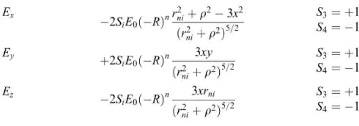
Table 3.Layer-1 secondary field terms for the HED

Ex

ÿ2SiE0…ÿR†n

r2

ni‡q2ÿ3x2 …r2

ni‡q2†

5=2

S3ˆ ‡1

S4ˆ ÿ1

Ey _‡

2SiE0…ÿR†n

3xy …r2_ni‡q2_†5=2

S3ˆ ‡1

S4ˆ ÿ1

Ez _ÿ

2SiE0…ÿR†n

3xrni …r2

ni‡q2†

5=2

S3ˆ ‡1

(Note that the second summation is only taken over iˆ3 and 4 in this situation. Except for the sign and a factor of two, the formulas in Table 3 are the same as those in Table 2.)

5 The vertical electric dipole

The vertical electric dipole ( VED) is taken to be z-directed (i.e. z-directed downwards) and located at the point (0,0,h). Otherwise the situation is as described in Sect. 2.

Because, in this case, there is complete azimuthal symmetry, the field formulas are less involved than is the case for the HED. The boundary conditions can be satisfied with a single-component Hertz vector Pzi…iˆ1;2;3† in each of the three layers, which is written in the same form as that for Pxi for the HED. Initially it is advantageous to use cylindrical polar co-ordinates …q;u;z†. The cylindrical polar components evaluated using Eqs. (1) and (2) are, explicitly:

Eqˆ @2Pz=oqoz;Ezˆ k2‡ @

2

@z2

Pz;Huˆ ÿr3@Pz=@q;

…22† all other field components being zero. The boundary conditions for the VED thus reduce to the continuity of k2Pz andoPz=ozacross each of the two interfaces. The solution for the VED at dc then proceeds analogously to that for the HED and we will not detail the algebraic processes involved here.

5.1 VED dc fields in layer 2

It is found that, at dc, the Hertz vector in layer 2 is expressible in the form of Eq. (10a) with

P…_z1₂†ˆ ÿMX

1

nˆ0 ÿRjj₂₃

n  r2

n1‡q2 q

; …23a†

P…_z2₂†ˆ ‡MX

1

nˆ1 ÿRjj₂₃

n  r2_n2‡q2 q

; …23b†

P…_z3₂†ˆ ‡MX

1

n_ˆ1 ÿRjj₂₃

n  r2n3‡q2 q

; …23c†

P…_z4₂†ˆ ÿMX

1

nˆ1 ÿRjj₂₃

n  r2

n4‡q2 q

; …23d†

from which the field components in layer 2 can be computed using Eq. (22). The results are presented in Sect. 6.1.

5.2 VED dc fields in layer 1

In layer 1, it is found that Pz1 may be written as

[compare Eq. (19) for the HED, noting that r 1P1ˆ @Pz1=@z]:

Pz1ˆ2M "

X1

nˆ0 ÿRjj₂₃

n  r2_n3‡q2 q

ÿX1

nˆ1 ÿRjj₂₃

n  r2

n4‡q2

q #

: …24†

In Eqs. (23) and (24) the rni (with iˆ3;4) are defined following Eq. (12). In Eq. (22), for layer 1;r30 at dc (andPz1is finite). It follows thatHuis zero in this layer. This is to be expected from Amperes law, because of the symmetry and the fact that there are no currents in layer 1. The electric field components, as computed from Eqs. (22) and (24) are presented in Sect. 6.2.

6 Recipes for computing the VED dc field components

6.1 DC VED fields in layer 2

The formulas for the VED fields in layer 2 are listed in Tables 4 and 5. The results in Table 4 are those of Table 1 modified for a z-directed dipole. Computation proceeds exactly as described in Sect. 4.1 except that Tables 4 and 5 are used in place of Tables 1 and 2, respectively. The cylindrical polar components …Eq;Bu; Ez†should first be calculated to the precision required. Finally, if needed, the Cartesian components may be computed from these using the relations presented in Table 4.

Table 4.Layer-2 primary fields of the VED

EqˆE03q…zÿh†=D5

EzˆE0 ‰3…zÿh†2ÿD2Š=D5

BuˆB0q=D3

ExˆxEq=q :EyˆyEq=q

Bxˆ ÿyBu=q :ByˆxBu=q:Bzˆ0 E0ˆ106 Id`=…4pr2† …givingEinlV=m†

B0ˆ100Id` …givingBin nT†

D2ˆq2 _{‡ …zÿh†}2_;

q2_ˆx2_‡y2

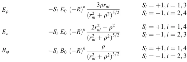
Table 5.Layer-2 secondary field terms for the VED

Eq ÿSiE0…ÿR†n

3qrni …r2

ni‡q2†

5=2

Siˆ ‡1;iˆ1;3 Siˆ ÿ1;iˆ2;4

Ez ÿSiE0…ÿR†n

2r2

niÿq2 …r2

ni‡q2†

5=2

Siˆ ‡1;iˆ1;4 Siˆ ÿ1;iˆ2;3

Bu ÿSiB0…ÿR†n

q

…r2

ni‡q2†

3=2

Siˆ ‡1;iˆ1;4 Siˆ ÿ1;iˆ2;3

ForEx;Ey;BxandBy use the formulas in Table 4; E0;B0andqare as defined in Table 4;

Rˆ…r3ÿr2†=…r3‡r2†.

rn1ˆ2nd‡h‡z; rn2ˆ2ndÿh‡z;

6.2 DC VED fields in layer 1

In layer 1 there are no magnetic field components for the VED (i.e. Bˆ0) so only the electric fields have to be computed. Computations of the electric field compo-nents are made following the procedure described in Sect. 4.2 using theE-field formulas of Tables 4 and 5 as follows.

To compute the sum of the primary plus thick-layer contribution use Table 4, multiplying each of the two electric field components by two. Then add on the result of the summation overnforiˆ3 and 4 (as in Sect. 4.2c) using the E-formulas of Table 5, but again multiplying each field component in Table 5 by two.

7 Specimen calculations and validation

7.1 Specimen Calculations

Specimen calculations for the HED and the VED gave the results presented in Table 6. A single precision algorithm was used and the computation terminated automatically (e.g. atnˆ31 for the layer 2 fields for the HED when the largest field component increment was, at most, 0:5210ÿ5 the existing value of that component)

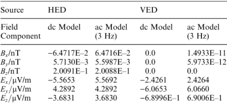
7.2 Validation

We have tested the dc formulas presented in this paper against our ac model (Burke and Jones, 1993, 1994), which had previously been programmed. This process checks the analytic derivations of the field components from the Hertz vector for the two cases and the resulting computer code. Clearly, the ac model should give the

same results as the dc model at sufficiently low frequencies. We have thus made computations using the dc model and the ac model at a frequency of 3 Hz. The results of the dc calculations and the modulus of the ac values for the various components in layer 1 are given in Table 7. The phase of the ac components (0 orp) also corresponds to the sign of the dc value. The dc and low-frequency ac fields in layer 2 also agreed numerically.

Acknowledgements. The work described here has been supported, in part, by the U.K. Defence Research Agency, Winfrith New-burgh, UK. Topical Editor D. J. Webb thanks S. Lovell and P. R. Bannister for their help in evaluating this paper.

References

Abramowitz, M., and I. A. Stegun, Handbook of Mathematical Functions, Dover Publications, New York, 1968.

Bannister, P. R.,New Simplified Formulas for ELF Subsurface-to-Subsurface Propagation, IEEE J. Ocean. Eng., OE-9,154–163, 1984.

Burke, C. P., and D. Ll. Jones,Electromagnetic Wave Propagation in Three-Layered Media,Technical Report RP921015, 1992.

Burke, C. P., and D. Ll. Jones, ELF Propagation in Deep and Shallow Sea Water, AGARD Conf. Proc. 529, AGARD (NATO), Neuilly sur Seine, France, pp 11.1–11.8, 1993.

Burke, C. P., and D. Ll. Jones,A Signal-to-Noise Model for ELF Propagation in Sub-Surface Regions, IEEE J. Ocean. Eng.,19,

353–359, 1994.

Chave, A. D., and C. S. Cox,Controlled Electromagnetic Sources for Measuring Electrical Conductivity Beneath the Oceans,J. Geophys. Res.,87,5327–5338, 1982.

Fraser-Smith, A. C., A. S. Inan, O. G. Villard and R. G Joiner,

Seabed Propagation of ULF/ELF Electromagnetic Fields from Harmonic Dipole Sources Located on the Seafloor,Radio Sci.,

23,931–943, 1988.

Kraichman, M. B., Handbook of Electromagnetic Propagation in Conducting Media, U.S. Government Printing Office, Washing-ton, DC 20402, Stock No. 008-040-00074-5, 1976.

Molchanov, O. A., Yu. A Kopytenko, P. V. Voronov, E. A. Kopytenko, T. Matiashvili, A. C. Fraser-Smith, and A. Bernardi,

Results of ULF Magnetic Field Emission Near the Epicenter of Spitac (Msˆ6:9) and Loma Prieta (Msˆ7:1) Earthquake, A Comparative Analysis, Geophys. Res. Lett., 19, 1495–1498, 1992.

Parrot, M., A. C. Fraser-Smith, O. A. Molchanov, and T. Yoshino,

Electromagnetic effects associated with earthquakes and volca-nic eruptions, EOS Trans. Am. Geophys. Union, 76,233, 1995.

Sommerfeld, A., Partial Differential Equations in Physics, Aca-demic Press, London, New York, 1967.

Table 6.Specimen calculations

Fields in Layer 2

Parameters:Id` ˆ1 Am,r2ˆ4 S/m,r3=r2ˆ0:15,hˆ2:0 m,

dˆ13:0 mx;y;zˆ50:0,)100.0, 11.0

HED – Number of terms used = 31. Relative Tolerance = 0.5E–05

Bx;By;Bz=pT = 0.60937 )2.4926 )7.0864

Ex;Ey;Ez/nV/m = 57.826 )118.01 5.5129 VED – Number of terms used = 35.Relative Tolerance = 0.50E–05

Bx;By;Bz=pT = 0.11092 5.54601E–02 0.00 Ex;Ey;Ez/nV/m =)0.98227 1.9645 )0.39477 Fields in Layer 1

Parameters:Id` ˆ1 Am,r2ˆ4 S/m,r3=r2ˆ0:15,hˆ2:0 m,

dˆ13:0 m x;y;zˆ5:0,)10.0,)10.0

HED – Number of terms used = 13. Relative Tolerance = 0.5E–05

Bx;By;Bz=pT = 62.946 88.785 )226.66

Ex;Ey;Ez/nV/m =)7803.4 )5157.0 )6514.0 VED – Number of terms used = 24. Relative Tolerance = 0.1E–06

Bx;By;Bz=pT = 0.00 0.00 0.00

Ex;Ey;Ez/nV/m =)5945.2 11890.4 5164.4

Table 7.Validation of dc model against the ac model (layer 1)

Source HED VED

Field Component

dc Model ac Model (3 Hz)

dc Model ac Model (3 Hz)

Bx/nT )6.4717E–2 6.4716E–2 0.0 1.4933E–11

By/nT 5.7130E–3 5.5987E–3 0.0 5.9733E–12 Bz/nT 2.0091E–1 2.0088E–1 0.0 0.0 Ex=lV/m )5.5653 5.5692 )2.4261 2.4264

Ey=lV/m 4.2892 4.2892 )6.0653 6.0660

Stratton, J. A.,Electromagnetic Theory, McGraw-Hill, New York, 1941.

Wait, J. R., Geo-Electromagnetism, Academic Press, London, New York, 1982.

Wait, J. R.,Electromagnetic Wave Theory, John Wiley, New York 1987.

Wait J. R.,Basic Radiation Fields, Radiosci.,4 (No. 4), 90–94, 1993.